Ground and Satellite-Based Methods of Measuring Deformation at a UK Landslide Observatory: Comparison and Integration

Abstract

With the advances of ESA’s Sentinel-1 InSAR (Interferometric Synthetic Aperture Radar) mission, there are freely available remote sensing ground deformation observations all over the globe that allow continuous monitoring of natural hazards and structural instabilities. The Digital Environment initiative in the UK aims to include these remote sensing data in the effort at forecasting and mitigating hazards across the UK. In this paper, we present a case study of the Hollin Hill landslide in North Yorkshire where a variety of ground-based geophysical measurements are available for comparison with InSAR data. To include Sentinel-1 data in the UK’s Digital Environment, it is important to understand the advantages and limitations of these observations and interpret them appropriately. The Hollin Hill landslide observatory (HHLO) is used by the British Geological Survey to understand landslide processes, and to trial new technologies and methodologies for slope stability characterisation and monitoring. In July 2019, six corner reflectors were installed to improve the coherence of the InSAR measurements. We use Sentinel-1 InSAR data acquired between October 2015 and January 2019 to study the behaviour of this landslide, and find that the line-of-sight component of the down-slope movement is 2.7 mm/year in the descending track, and 7.5–7.7 mm/year in the ascending track. The InSAR measurements also highlight the seasonal behaviour of this landslide. Using InSAR data after the installation of the six corner reflectors, we are able to track the most recent movement on the landslide that occurred in January 2021. This result is in agreement with other ground-based measurements such as tracking of pegs, and soil moisture data derived from electrical resistivity tomography.

1. Introduction

The InSAR (Interferometric Synthetic Aperture Radar) technology is widely used for measuring millimetre-scale deformation of the Earth’s surface [1], and applications are widespread from monitoring natural hazards, such as volcanoes (e.g., [2]), earthquakes (e.g., [3]) and landslides (e.g., [4]), to structural engineering applications, such as monitoring subsidence (e.g., [5]) and structural stability (e.g., [6]). The Sentinel-1 constellation provides freely available InSAR measurements over the globe, repeating every 6 or 12 days. This allows regular monitoring of various potential hazards anywhere on Earth. However, InSAR comes with limitations: it gives a measurement of relative displacement, and it is prone to errors due to atmospheric variations and the type of land cover that is present in the area of interest. This relative displacement is measured in the one-dimensional line-of-sight direction, but multiple look angles with different line-of-sight directions give better coverage. One way to obtain reliable InSAR results is to compare them with ground-based measurements and interpret them with other information we might know about the area and geology.

The British Geological Survey (BGS) maintains the National Landslide Database in the UK [7]. This database holds over 17,000 records, and it is continuously updated from various sources, including BGS geological maps, active surveys, research studies and information from the public.

Yearly financial losses due to landslides are likely to be considerably in excess of 10 million GBP [8]. Each landslide can be unique in its behaviour; some move slowly and continuously, while others are inactive for years and then move episodically. Often landslides are triggered by excessive rainfall, like the Hollin Hill landslide. With the UK’s climate predicted to be wetter and more varied according to the the UK Climate Projections 2018 (https://www.metoffice.gov.uk/research/approach/collaboration/ukcp/index last accessed on 13 August 2021), landslide activities could become more and more frequent. A 2013 study indicated that the wettest year on record until then, 2012, coincided with a four- to five-fold increase in landslide activities compared to previous years [9].

In this paper, we present a case study of the Hollin Hill Landslide Observatory (HHLO) (Figure 1), where the British Geological Survey has developed and established ground-based geophysical monitoring systems [10,11], supplemented with ground-based geotechnical and displacement sensors and airborne (drone and conventional aircraft) repeated surveys. The Hollin Hill landslide is one of the best studied slow-moving landslides in the world (e.g., [12,13,14,15]) and the available ground-based measurements make it an exceptional location to study the InSAR measurements in comparison with the established ground truth data.

We compare these geophysical and displacement data from the ground that we consider ground truth with InSAR displacement and velocity results derived from satellite-based Sentinel-1 measurements, and interpret them together to study the behaviour of this landslide. Interpretation of InSAR data over vegetated settings can be challenging, and in order to improve the SAR signal, six corner reflectors were placed on the Hollin Hill landslide in July 2019. We analysed the amplitude, phase and coherence signal of the SAR measurements before and after the installation, and show the improvement these reflectors provide in retrieving ground deformation.

The addition of InSAR measurements to the already existing ground-based geophysical observations can help provide consistent and comprehensive information on ground deformation for the entire slope. More generally, the analysis presented in this paper provides the basis for an integrated space–ground monitoring system that can support the identification and monitoring of these hazards. Understanding landslide behaviour is, in turn, an important step for retrieving their impact on the society.

2. Materials and Methods

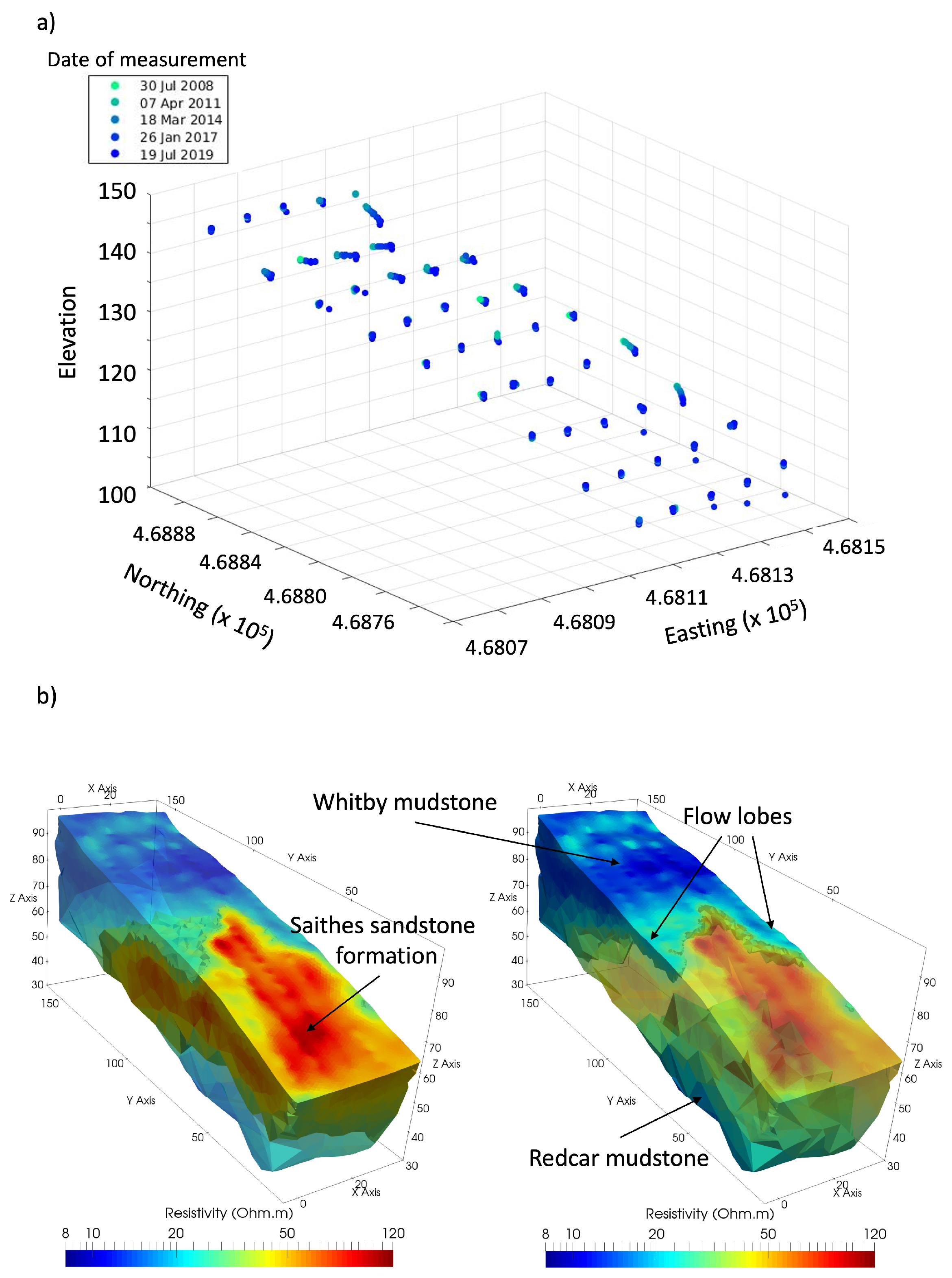
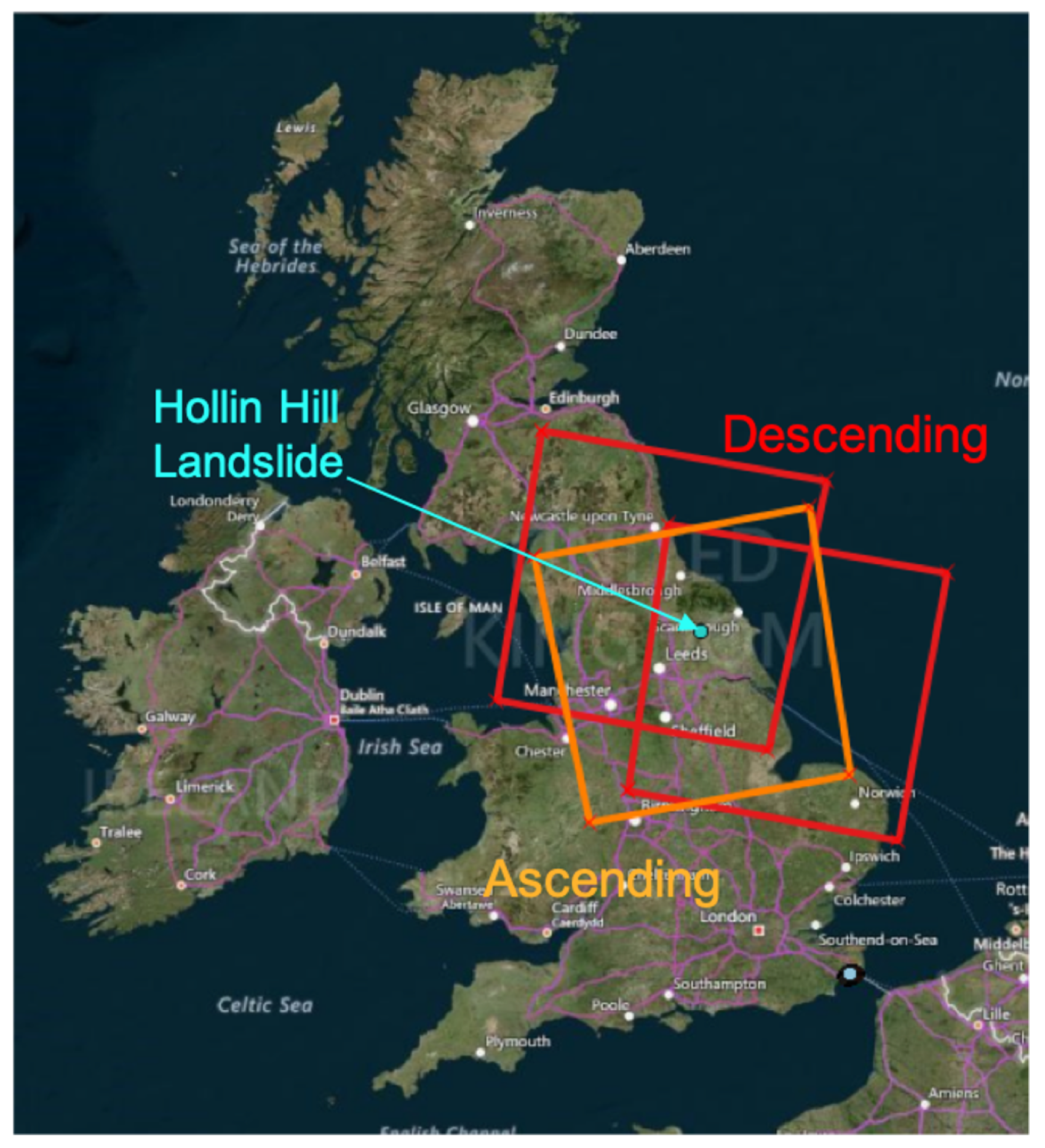
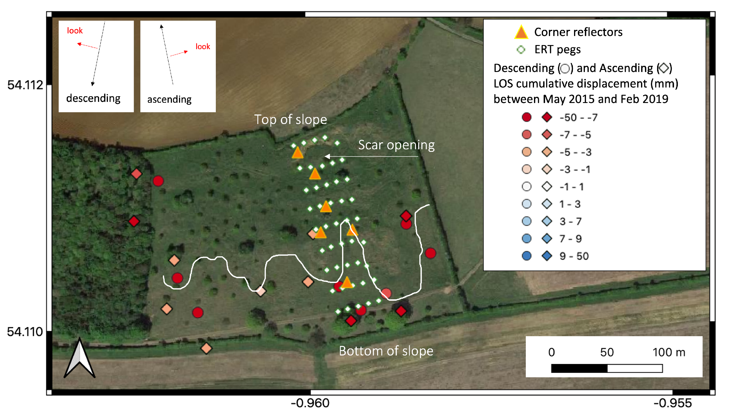
2.1. Site Description

The Hollin Hill Landslide Observatory (HHLO) is several hundred metres wide and extends 200 m down slope. It is located on a south-facing ∼12° slope and consists of the Redcar Mudstone (Lower Lias) at the base, with an outcrop of the Staithes Sandstone Formation (Middle Lias) running across the middle section of the slope. The Whitby Mudstone Formation (Upper Lias) overlies this, with the upper part of the slope composed of the Dogger Formation [16]. Movement across the entire slope is due to the Whitby Mudstone Formation which is highly susceptible to failure in this area. The landslide is characterised by shallow rotational failures at the top of the slope in the Whitby Mudstone. The rotational failures form as support is removed in the mid-slope, where the Whitby Mudstone approaches or exceeds its liquid limit, and is subject to deformation. Displacement material from the mid-slope “cascades” over the in situ Staithes Sandstone Formation, creating large (3–4 m vertical displacement) back scarps and feeding into four larger-scale slow-moving (i.e., tens of centimetres per year) flow lobes of slumped material at the bottom of the slope [17,18] (marked with white lines on Figure 2).

Landslide activity is typically governed by rainfall and soil moisture; in general, seasonal behaviour can be observed [19,20]. Periods of elevated soil moisture content induced by sustained effective rainfall, typically during the winter months (spanning from December to March in the UK) can trigger motion on the landslide in the order of centimetres to tens of centimetres [11]. In contrast, heavy/extreme isolated rainfall events occurring in periods of low antecedent moisture are not associated with movement on the slope [15].

2.2. Geophysical Data

HHLO is a well-studied landslide acting as a field laboratory managed by BGS to support UK landslide research. Ground-based geophysical methods are used to monitor the site, including 4D Electrical Resistivity Tomography (ERT). ERT as a monitoring tool can provide information about changes in the subsurface hydrological conditions [21], and is therefore highly relevant and increasingly used to track precursors of slope failure in moisture-induced landslides [20]. In the spring of 2008, an Automated Time-Lapse Electrical Resistivity Tomography (ALERT) system was permanently installed on the site [22,23]. The ALERT instrument uses wireless telemetry (in this case GPRS) to communicate with a computer in the office, which runs control software and a database management system. The resulting daily electrical resistivity models can be transferred to models of Gravimetric Moisture Content (GMC) distribution using the Waxmann–Smits relationship [24]. At the HHLO, this is done using the approach developed by [11]. The ERT measurements are complemented by tilt data and displacement data from shape acceleration arrays, as well as from a network of GNSS marker pegs repeatedly surveyed on a quarterly basis with real-time kinematic (RTK)-Global Navigation Satellite Systems (GNSS). In 2020 the ALERT system was replaced by a PRIME system [25]. The ERT measurements are also adjusted so that the movement of the pegs with the landslide is taken into account when modelling the resistivity in the subsurface [15]. Additionally, measurements of temperature, humidity, precipitation, solar radiation, wind speed and volumetric water content are being continuously recorded by a weather station from the UK Cosmic-Ray Soil Moisture Observing System (COSMOS, https://cosmos.ceh.ac.uk/ accessed on 8 June 2022) network [26,27].

These ground-based measurements are also complemented by airborne surveys; BGS have been flying drone surveys repeatedly since 2014. Ground displacement has also been monitored through terrestrial LiDAR and drone photogrammetry surveys acquired yearly since 2014. A more detailed monitoring program of drone photogrammetry surveys has also been undertaken since [18,28]. LiDAR data were acquired from conventional aircraft in 2011.

Figure 2 shows the location of the pegs that mark the old ERT survey (white diamonds) in use until late 2020, and InSAR velocities in line-of-sight (LOS) direction between May 2015 and February 2019 (circles and diamonds). The peg survey is laid out with a spacing of ∼10 m across the slope and of ∼20 m down the slope. The InSAR velocities are relative compared to a stable reference area nearby. The white line marks the extent of the flow lobes. The motion of these pegs between 2008 and 2019 shows both a rotational back scarp that has opened at the top of the slope, as well as motion around the middle of the slope that can be associated with the flow lobes identified with the ERT measurements (Figure 3).

Results of the ERT survey show that the Staithes Sandstone Formation in the middle has the highest resistivity, compared to the overlying Whitby Mudstone Formation and underlying Redcar Mudstone Formation [29]. The largest movement on the slope is measured at the top and easternmost side where a scar has opened, visible on satellite images (Figure 2) and lateral displacements up to 8.6 m between 2005 and 2018 [15]. Flow lobes, comprising a slipped Whitby Mudstone Formation, are observed towards the base of the slope; these are marked with white lines on Figure 2.

3. Results

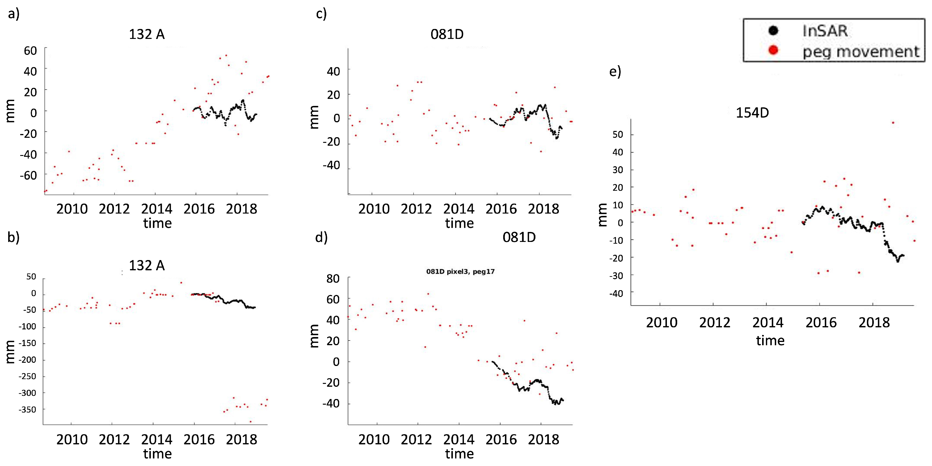
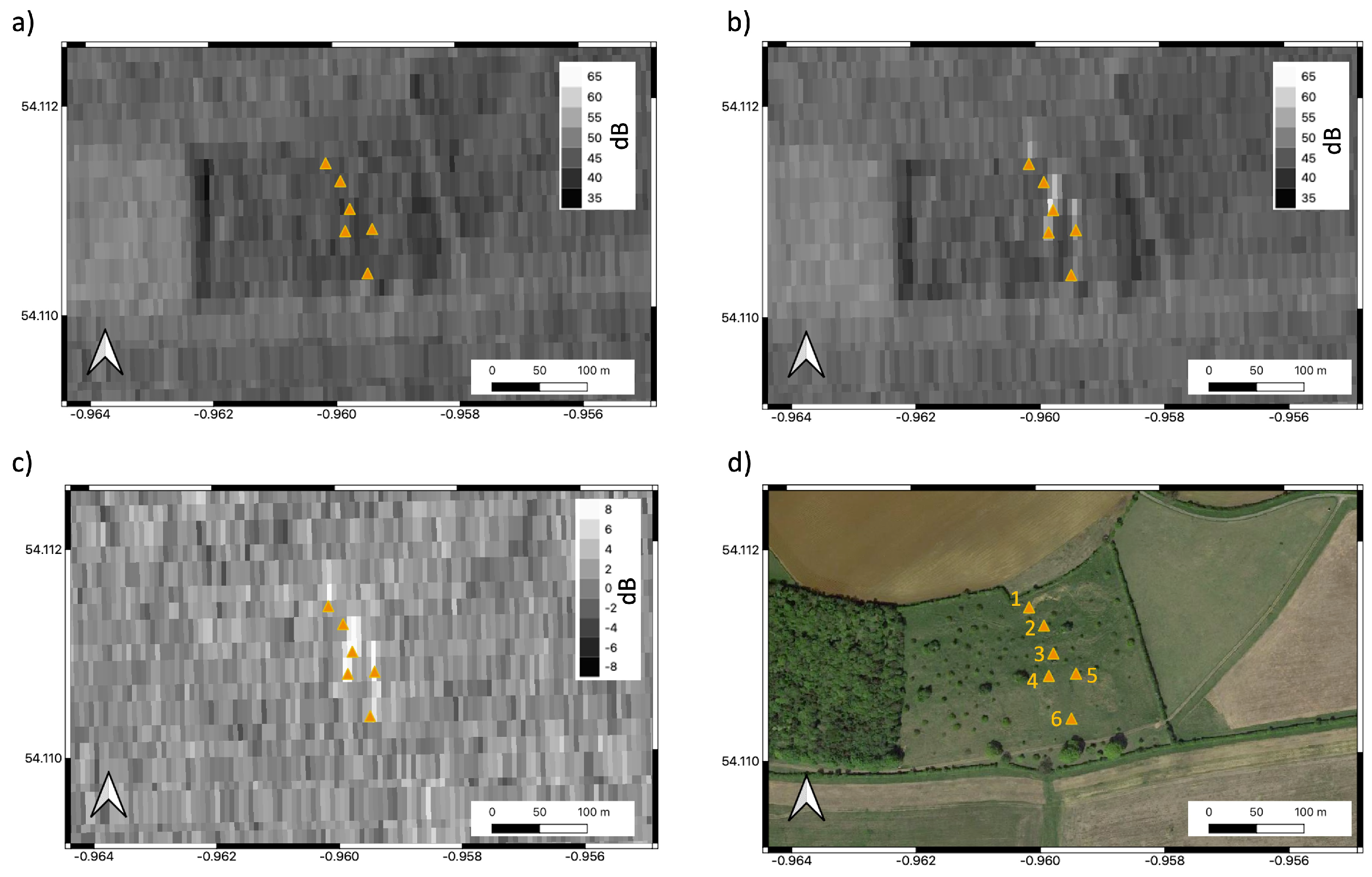
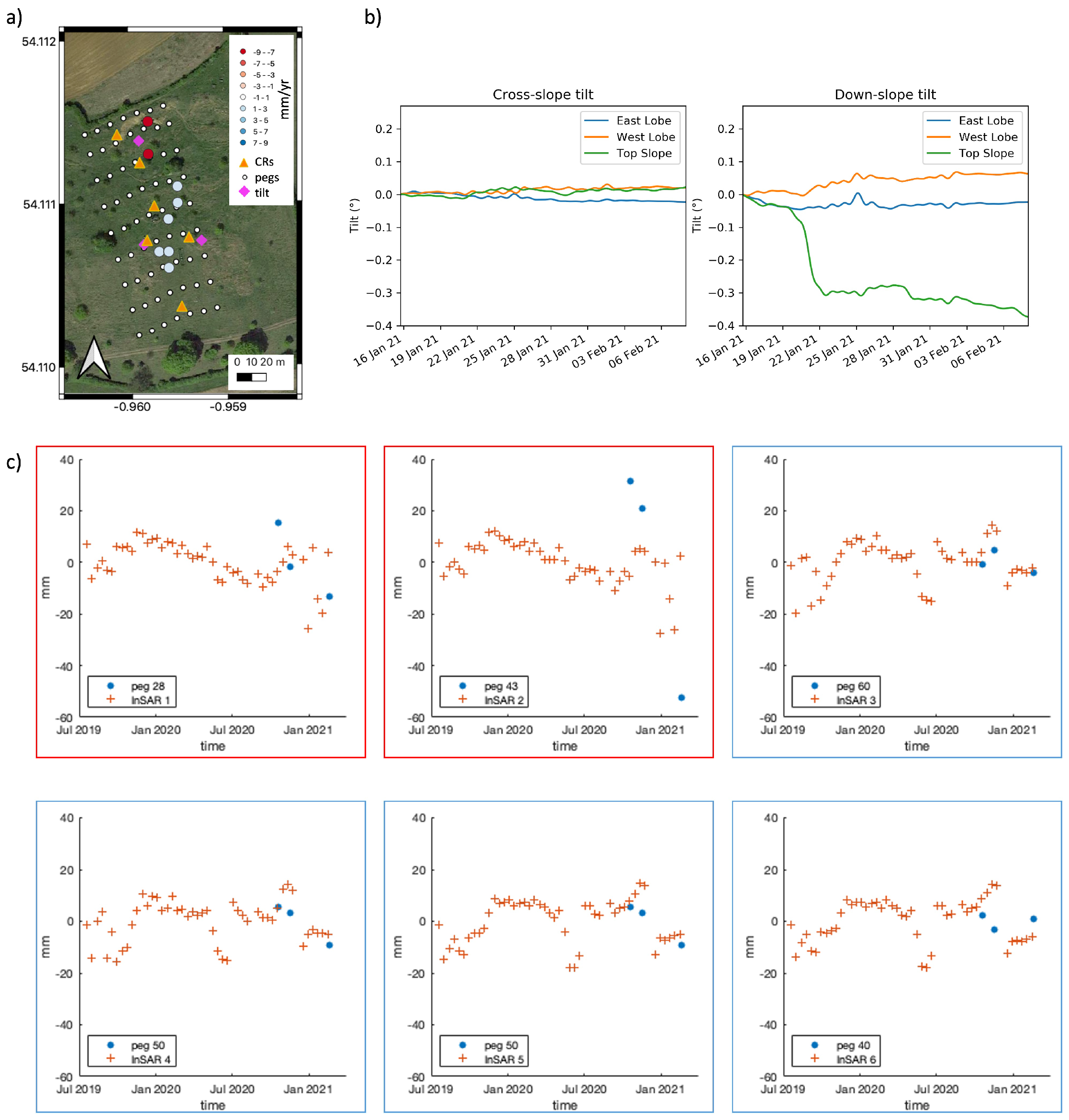
3.1. InSAR Data and Corner Reflectors

So far, no InSAR study has been done at the HHLO due to limitations in temporal resolutions of previous SAR constellations and the vegetation cover on the ground. It is challenging to assess vegetated settings with InSAR due to noise from loss of coherence between separate acquisitions (e.g., [30,31,32]). Additionally, potential biases can be introduced due to changes in soil moisture and/or vegetation over the time of measuring [33]. Still, the Hollin Hill landslide is representative of vegetation covered, slow moving landslides in the UK and it is one of the most extensively monitored landslide sites in the UK and therefore a good candidate area to validate InSAR results. Due to its orientation towards the south and movement along the slope, the horizontal component is challenging to capture with the ascending configuration of the Sentinel-1 SAR mission.

We analyse InSAR results in two different ways in this paper: (1) establishing long-term trends using the available span of the Sentinel-1 data since 2015, and (2) analysing the improvement that the installation of corner reflectors achieved in July 2019.

We use the available InSAR data from the Sentinel-1 mission processed by SatSense [34]. The data processing reduces the noise of the InSAR measurement due to atmospheric effects and filters the displacement time series in order to reduce effects of overall temporal noise. We use these velocities and displacement time series to assess the motion of the landslide during the time span of the Sentinel-1 mission, between October 2015 and January 2019.

In July 2019, we installed six trihedral triangular corner reflectors made of aluminium with 0.7 m edge and a thickness of 3 mm. They are all oriented towards the ascending geometry and anchored to the ground with sand bags and a concrete slab. We chose the ascending direction because the R-Index map showed that the ascending geometry is more suitable than the descending one [35]. In our design, the reflectors can be rotated 360° in azimuth and the baseplate can be elevated between 0 and 40° (with respect to the horizontal ground surface). From these characteristics, they are able to provide an RCS of about 1300 m² (i.e., 16 dB) with Sentinel-1 C-band acquisitions [36].

They are located in the same area as that equipped with the geophysical and geotechnical monitoring systems, which will facilitate comparisons of the ground-based and remote sensing tools (Figure 2). From north to south, the corner reflectors are located on (1) stable zone (behind back scar), (2) rotational zone, (3) sub-rotation (translational zone), (4) west flow lobe, (5) east flow lobe and (6) stable zone (valley between flow lobes). We would expect these areas to move at different rates and times. The locations of the corner reflectors are shown in Figure 2.

We processed Sentinel-1 InSAR data from July 2018 to May 2021 in order to study the effect of the corner reflectors. We used the Gamma-based [37] LiCSAR processing chain for co-registering the 85 ascending acquisitions of Path 132 and Frame 172 [38].

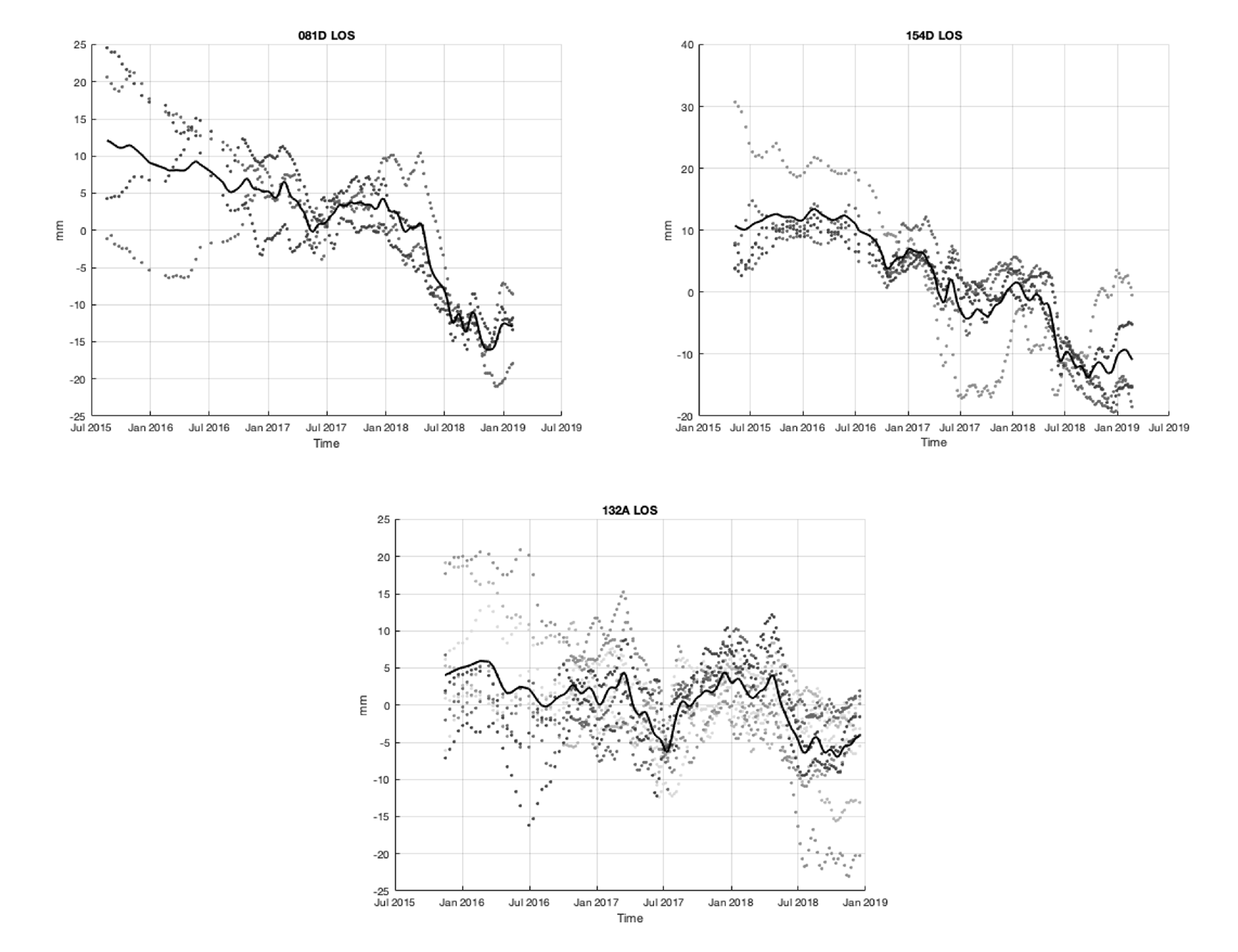
3.2. InSAR Results before the Installation of Corner Reflectors

The location and line-of-sight velocity over the analysed time period are shown in Figure 2 with diamonds and circles representing ascending and descending measurement points, respectively. We analysed InSAR data from three Sentinel-1 frames: one ascending (132) and two descending (081 and 154). The number and distribution of these InSAR measurements are typical of a vegetated setting in the UK but they are not ideal for detailed monitoring of a moving slope. Good quality scatterers were not available until the July 2019 deployment of corner reflectors and therefore InSAR measurements that are coherent enough for interpretation are located sparsely.

The individual time series of displacement in the line-of-sight direction are shown in Figure 4. These time series are locally re-referenced to a stable area approximately 1 km north from the slope and show displacement relative to this stable area.

Both descending and ascending time series capture the seasonal behaviour of this landslide due to wetting in the winter months and drying during the summer months. In the descending time series, the movement of the landslide down slope is more apparent than in the ascending case, which appears to be noisier and to coincide less with the moving parts of the slopes than the descending points. This is consistent with the down-slope direction being perpendicular to the ascending line of sight. The mean line-of-sight component of the mean subsidence rate measured with the 132 ascending frame is 2.7 mm/year, while with the 081 descending and 154 descending frames it is 7.7 mm/year and 7.5 mm/year, respectively. The nominal error on these values is 1 mm/year [39].

We selected the pixels that are closest to individual pegs and compared the displacement of the ERT pegs with the InSAR measurements. Coherent InSAR pixels can only be found towards the south end of the slope in the area where the peg survey is placed. For this comparison we converted the displacement measured at the location of the pegs into line-of-sight direction of the corresponding InSAR acquisition (Figure 5).

The varying agreement of the individual InSAR displacement time series and the ground-based measurements show that the Hollin Hill landslide is a challenging area for InSAR measurements due to its grass cover, aspect, and lack of reflective objects. The average displacement time series for each track, however, is more representative of the overall down-slope motion and seasonal behaviour of the landslide. This seasonal behaviour is not as apparent on the ERT peg measurements as on the average InSAR displacement time series (black lines in Figure 4).

In the descending time series, a drop can be seen in 2018; this is due to activity on the landslide during this time. There was a reactivation of the back scarp that also resulted in displacement on the flow lobes. The InSAR time series in Figure 4 and Figure 5 reflect the motion on the flow lobes; their location is shown in Figure 2.

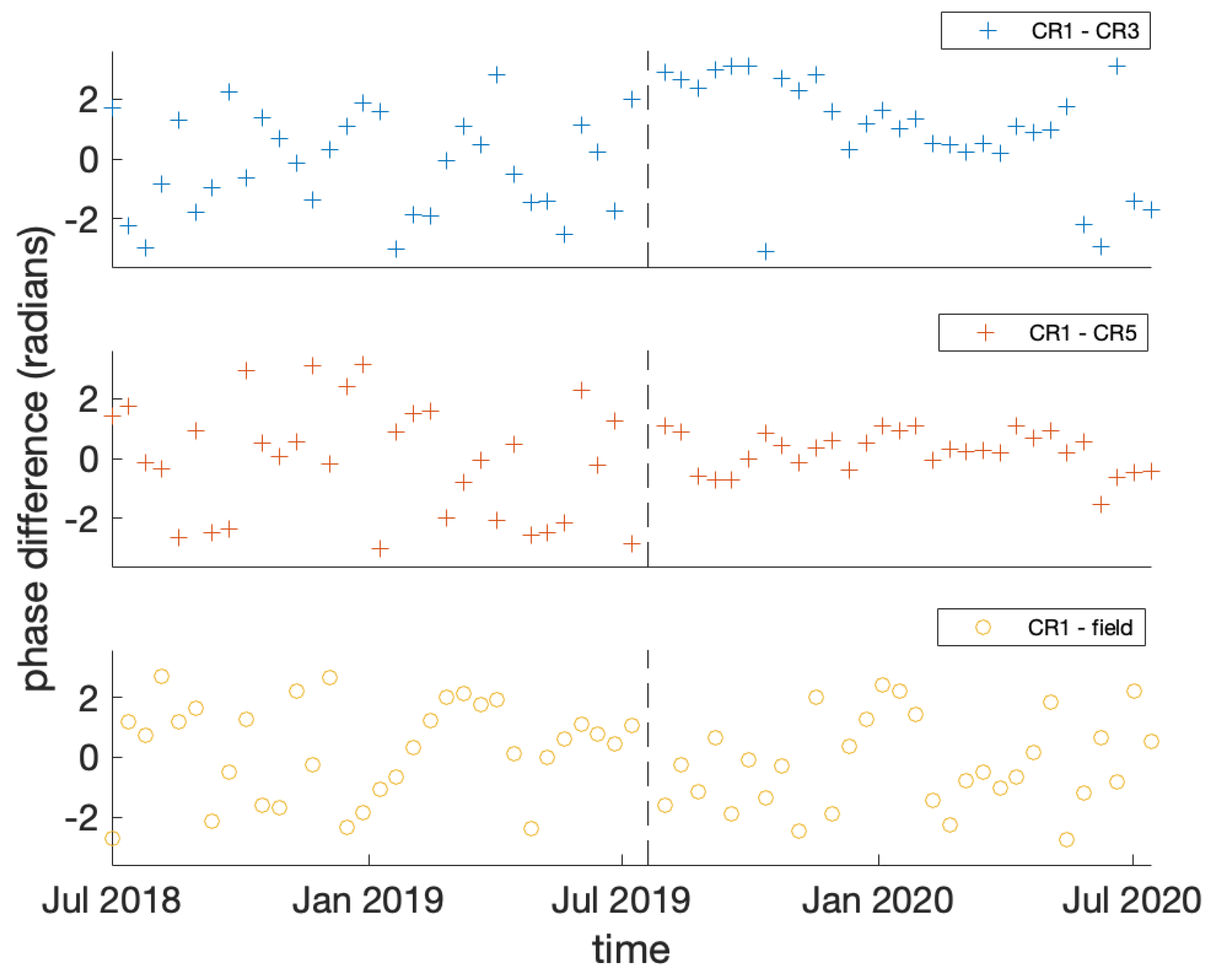
3.3. InSAR Results after the Installation of Corner Reflectors

Six corner reflectors were installed in July 2019 in order to enable recordings of more coherent InSAR measurements. The improvement in the intensity of the InSAR measurements at the locations of the corner reflectors is shown in Figure 6. We averaged the intensity of the images before and after the installation of the corner reflectors using the co-registered SLCs, and then calibrated and geocoded the resulting amplitudes.

Figure 7 shows phase analysis of individual pixels extracted from ascending interferograms that have been created with the same master date (20 July 2019). The northernmost reflector (CR1) was chosen as a reference point; this is above the back scarp at the top of the landslide. We plot the difference in phase between this reference corner reflector and two other reflectors and find that the phase signal is more stable than before the installation of the corner reflectors (Figure 7). For reference, we include a plot of phase difference between the reference corner reflector and a random point in the field of the Hollin Hill landslide.

We calculated the standard deviation of the displacement for each pixel containing a corner reflector with reference to a nearby stable area (

Table 1. Standard deviation of displacement accuracy (mm) values corresponding to each pixel with a corner reflector in it. We show these results over a four month period (top rows) and over a year (bottom rows) before and after the installation of the corner reflectors.

Setup	CR1	CR2	CR3	CR4	CR5	CR6	Time Period
Before	9.07	6.01	9.02	7.31	5.03	10.21	April 2019–July 2019
Before	8.30	6.65	8.82	5.99	7.18	8.76	July 2018–July 2019
After	1.65	8.91	1.33	1.71	1.98	7.86	August 2019–November 2019
After	4.62	7.83	9.50	7.30	3.48	8.25	August 2019–August 2020

). We see improvement in the standard deviation of CRs 1, 3, 4, and 5 over a 4 month period, while no clear improvement can be seen over the year-long time period. This is most likely due to seasonal variations that become more prominent when assessing time periods over seasons with significant changes in vegetation. CRs 2 and 6 appear to have smaller amplitudes in Figure 6 and these also do not have an improvement in the standard deviation of displacement accuracy. CR2 is located on the rotated block of the landslide. This area experiences a very different deformation regime to the rest of the slope—while other areas slide horizontally and downhill, CR2 is in a location that probably experiences more uplift and tilt, but potentially less movement down slope. The surface in this area is the most affected by large cracks because of the uplift and hydrological de-coupling from the underlying ground, which could be the explanation for the poorer performance of CR2.

In addition to amplitude and phase analysis, we also calculated the coherence of each pixel containing a corner reflector (1) from Pepe et al. (2006) [40]

$$\gamma =\frac{\left|{\sum }_{p=0}^{M-1}exp\left[j\left({\phi }_p-{\overline{\phi }}_p\right)\right]\right|}{M},0\le \gamma \le 1$$

(1)

calculating the $\gamma$ coherence for each corner reflector using the M number of measurements and the $j\left({\phi }_p-{\overline{\phi }}_p\right)$ phase difference between the reference epoch (the first acquisition date after the installation of the corner reflectors) and all other measurement epochs.

Table 2. Coherence values corresponding to each pixel containing a corner reflector. We show coherence results over a four-month period (top rows) and over a year (bottom rows) before and after the installation of the corner reflectors.

Setup	CR1	CR2	CR3	CR4	CR5	CR6	Time Period
Before	0.22	0.48	0.25	0.24	0.51	0.32	April 2019–July 2019
Before	0.05	0.43	0.36	0.44	0.13	0.13	July 2018–July 2019
After	0.92	0.07	0.95	0.94	0.95	0.73	August 2019–November 2019
After	0.46	0.16	0.49	0.57	0.79	0.21	August 2019–August 2020

shows the results of these calculations.

We observe the general improvement of coherence both over shorter periods of time (10 acquisitions over approximately 4 months) and over a full year of acquisitions that includes all seasons. When calculating the standard deviation of displacement accuracy and coherence over 4 months only, we see that four out of the six corner reflectors achieve an accuracy below 2 mm and coherence over 0.9, while two reflectors do not appear as accurate and coherent. These reflectors correspond to the ones that appear to have smaller amplitudes in Figure 6 (the second and sixth reflectors from north to south). The importance of the improved coherence and phase stabilisation is that, as noise is being removed, the displacement on the landslide can be estimated more accurately.

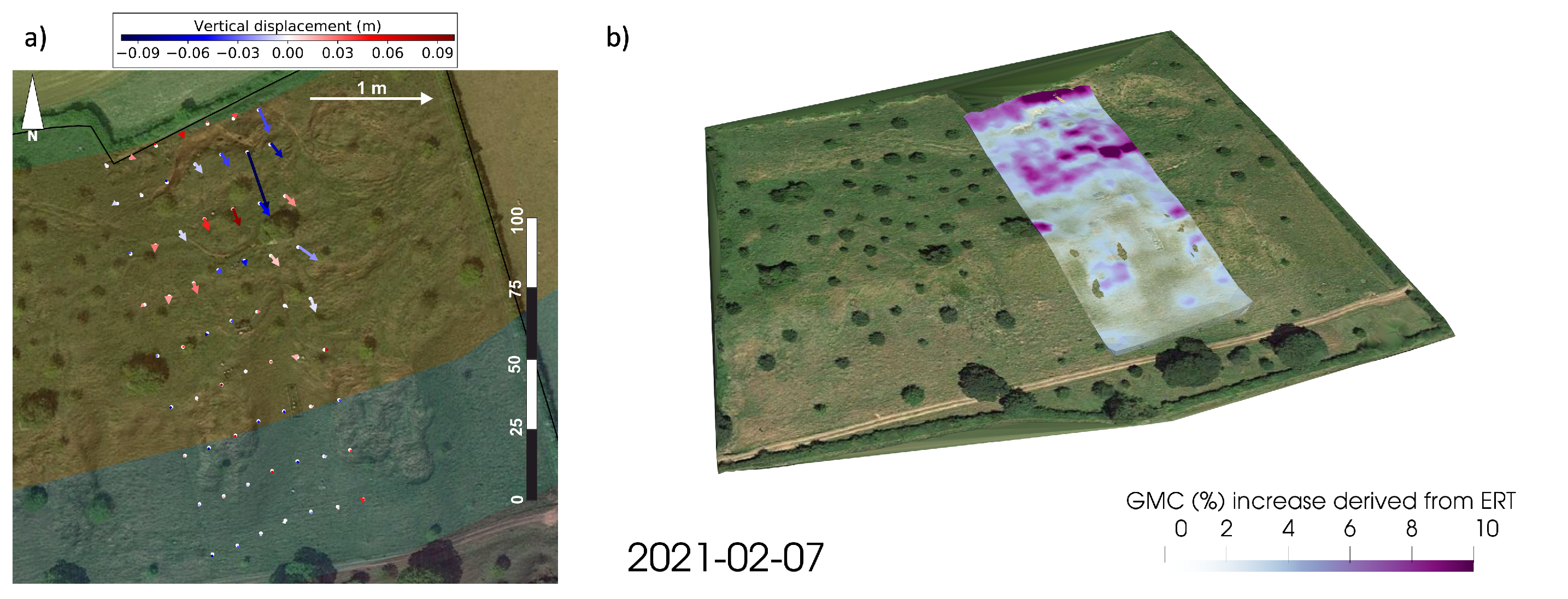
3.4. Movement on the Landslide in January 2021

After a long period of inactivity, the Hollin Hill landslide experienced some movement in January 2021. A new grid of marker pegs was installed on the landslide in November 2020 and surveyed with GNSS in the following months, capturing movement in January 2021. It appears that the related landslide event was confined to the upper part of the slope and did not extend to the lower flow lobes (Figure 8a). The movements measured on the marker pegs include horizontal displacements of up to 50 cm associated with vertical displacements of up to 10 cm. In the period preceding the event, the ERT-derived moisture content distribution highlights areas of elevated moisture content at the top of the slope in significantly higher proportions than in lower parts of the slope (Figure 8b).

We processed InSAR data since the installation of the corner reflectors using the LiCSAR system and we carried out time series analysis using the StaMPS package [41] on the coherent pixels located in the vicinity of the corner reflectors. None of the other pixels on the slope were coherent enough for this analysis, and while some geocoding error might be present, it is reasonable to assume that the reflections that give the coherent results come directly from the corner reflectors.

Based on the velocities derived from these coherent pixels, we find again that the movement during the 2021 January event was confined to the northern part of the slope and did not cascade down to the flow lobes and lower parts of the landslide (coloured dots in Figure 9a). Individual time series of these InSAR results show greater movement in the InSAR line-of-sight direction in the northernmost area of the slope around January 2021, as expected from the velocity analysis. We converted the GNSS results from the peg survey from 3D to the InSAR ascending line of sight and compared these with the InSAR time series (Figure 9b). While this line-of-sight component represents only one component of the movement, there is an agreement between the InSAR time series and the three GNSS measurements that were carried out before and after this event in January 2021.

In addition, we show time series of the three tiltmeters that were placed among the pegs in January 2021, only days before the movement on the landslide (Figure 9c). There are multiple measurements each day that range between a wide array of values due to the tiltmeters’ sensitivity to temperature. We apply a low-pass filter to smooth these daily variations. We observed tilting of the ground at the top of the slope on the 21st of January 2021. The tiltmeters on the west and east lobe do not show significant change at this time. These observations also confirm what we see with the pegs and the InSAR displacement time series: that the ground motion in January 2021 was confined to the top of the slope.

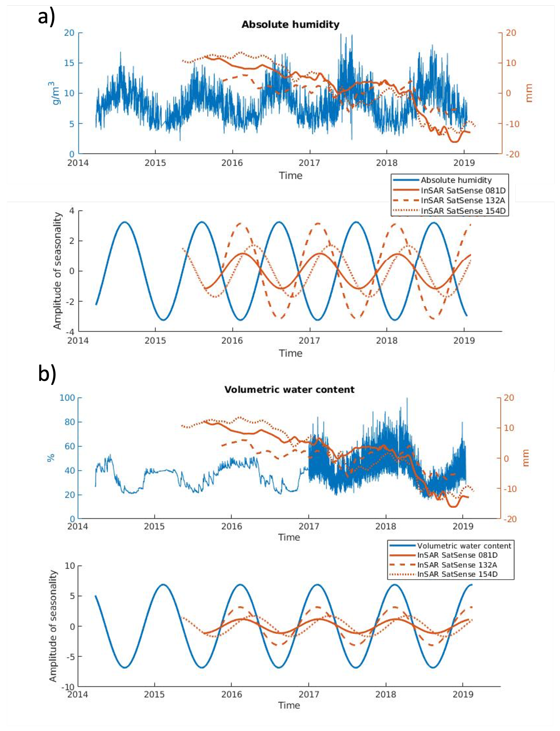
3.5. Relationship to Soil Moisture

It has been shown that the Hollin Hill landslide is going through episodic accelerations and can be triggered by elevated soil moisture levels, usually during the winter or spring months [11]. In regular years the landslide shows seasonal behaviour due to the wetting of the soil during winter and the slow drying during the summer. A reactivation of the landslide after years without significant movement happened in the winter of 2012/2013 after anomalously high levels of rainfall during two consecutive summers, with the summer of 2012 being the wettest of the last century [9,42]. During the winter of 2012/2013, rainfall was still 50% above the 30 year average [42], which led to the reactivation of the landslide. Similarly, the rotational back scarp at the top of the slope started developing in April 2016, following a particularly wet winter.

For the 2012/2013 event, observations of gravimetric moisture content show that during this period of unusually high rainfall and the reactivation of the landslide, the usual seasonal behaviour of the landslide changed [11]. We compared the ground-based measurements of absolute humidity and Volumetric Water Content (VWC) to the InSAR time series (top panels of Figure 10) and expanded on work done previously by comparing SAR and VWC [43]. Volumetric water content is the ratio of water volume to soil volume and it has been measured at the Hollin Hill site since March 2014 with the COSMOS system at a depth between 15 and 40 cm [44].

Using a sinusoid fit, we extracted the seasonal component of the absolute humidity, the volumetric water content and the InSAR time series measurements (bottom panels of Figure 10). We found that there is evidence for similar seasonal behaviour of the InSAR displacement measurements, especially with the VWC measurements. The seasonal fits extracted from the three different InSAR tracks differ slightly from each other, but they all peak in the same season, showing the same behaviour. The seasonal behaviour of the absolute humidity shows a lag in time compared to the InSAR time series results. Some studies suggest that soil moisture can introduce a bias in velocities derived from InSAR data (e.g., [45]), but further investigation is required to specify the extent of this effect at the Hollin Hill landslide.

Based on the ERT results and the latest movement detected on the landslide in January 2021, we can see another example of the relationship between soil moisture and the triggering of new events on the landslide. This particular event appears to be smaller than previous ones and confined to the top of the slope, which fits with the elevated moisture levels detected only on the upper half of the slope and the 2020/2021 winter not being exceedingly wet.

4. Discussion

The corner reflectors installed on the Hollin Hill landslide give us unprecedented additional information into the spatio-temporal behaviour of the landslide. The European Ground Motion Service (https://land.copernicus.eu/pan-european/european-ground-motion-service accessed on 8 June 2022) which provides InSAR data resampled at 100 m does not pick up any coherent points over the Hollin Hill landslide. Specific data processing with corner reflectors installed on a landslide therefore can give new insight into the behaviour of slow-moving landslides not only at Hollin Hill but also of landslides that are not studied so extensively with other geophysical methods.

Since the corner reflectors are placed on a moving slope (on Hollin Hill five out of six are on the landslide itself), their stability is a concern, as well as how to interpret the displacement signal, and whether it belongs to a deeper motion on the landslide or only a superficial one. A future analysis could study the displacement profiles in greater depth. Placing corner reflectors facing the descending geometry could also help disentangle the different components of the motion.

The COSMOS sensors (https://cosmos.ceh.ac.uk/sites/HOLLN, accessed on 8 June 2022) measure soil moisture at depths of −0.1 m and between −0.15 and −0.4 m [44] which are well below the penetration capabilities of the C-band SAR sensors. Deeper investigation of the signal that the InSAR analysis picks up could shed more light on whether it is coming from the top surface or a deeper source. This could also give constraints on the permeability of the soil, and whether the motion detected is more connected to rainfall or to soil moisture. Based on comparison between the soil moisture sensor and displacement measurements (from downhole shape accelerometer arrays), the Hollin Hill landslide requires a certain level of antecedent soil moisture (∼48% moisture [11]) before it will start to fail in response to large rainfall events. Even with some of the largest effective rainfall events in 2017, the site did not move; however, far smaller individual events triggered movement when there was a higher background moisture content in 2018.

With the work presented in this paper, we provide additional information concerning the spatio-temporal behaviour of the Hollin Hill landslide. Until now, only sparse GNSS measurements were available to try to understand the spatial variation in movement on the landslide. InSAR data bridge the time gaps between these GNSS surveys. We highlighted the importance of climate in controlling the motion on the landslide; however, further investigation is needed in understanding slow-moving landslides.

5. Conclusions

We analysed Sentinel-1 InSAR measurements over the HHLO from three frames, and compared them to ground-based measurements of GNSS locations, soil moisture derived from electric resistivity tomography, as well as absolute humidity and volumetric water content. We conclude that while individual displacement time series can be noisy, the average InSAR displacement time series capture the down-slope movement and the seasonal behaviour of the landslide in general. Due to the grass cover, lack of reflective objects and orientation of the slope, it is a challenging area to use InSAR measurements for monitoring the landslide, but as it is representative of the hundreds of landslides across the UK, this study can provide an insight into the feasibility of InSAR in such areas. We found that the observations from the descending tracks are less noisy and show the down-slope movement better than the observations from the ascending track. The corner reflectors that have been installed to face the ascending satellite might remedy this in the long term and produce better located and less noisy data from the ascending InSAR acquisitions. Corner reflectors facing the descending track would also enhance the accuracy of movement tracking on the slope. The most recent 2021 January movement on the top part of the landslide was captured by various ground-based and remote measurements, including the GNSS peg surveys, tiltmeters, elevated moisture contents derived from the ERT survey and InSAR time series based on the reflections from the corner reflectors. The movement that we detected is of the order of a few centimetres and therefore too small to be detected with the repeat LiDAR surveys.

In the future, we aim to process more Sentinel-1 data over the area of the Hollin Hill landslide and study the motion of the recently installed corner reflectors. We expect that the comparison with ground-based measurements, such as the movement recorded by the GNSS measurements of the pegs of the ERT survey, or the moisture recorded by the various instruments at the site, will improve, at least with the ascending acquisitions, due to the deliberate placement of the corner reflectors.

Future work is required to assess the applicability and utility of corner reflectors for active land sliding in the UK. According to the BGS National Landslide Database, there are over 17,000 landslides in the UK. Monitoring this large number of landslides is a challenge, and remote sensing techniques can play a great role in providing information. As we overcome limitations, such as temporal coverage with the Sentinel-1 mission or vegetation cover with the installation of corner reflectors, it will be more and more feasible to use the InSAR technology for continuous observation of the large number of landslides. Studies of landslides in, for example, Italy [46] and Norway [47] show improvement in the understanding and monitoring capabilities with corner reflectors installed.

References

1. Bamler, R.; Hartl, P. Synthetic aperture radar interferometry. Inverse Probl. 1998, 14, R1. [Google Scholar] [CrossRef]
2. González, P.J.; Bagnardi, M.; Hooper, A.J.; Larsen, Y.; Marinkovic, P.; Samsonov, S.V.; Wright, T.J. The 2014–2015 eruption of Fogo volcano: Geodetic modeling of Sentinel-1 TOPS interferometry. Geophys. Res. Lett. 2015, 42, 9239–9246. [Google Scholar] [CrossRef] [Green Version]
3. Delouis, B.; Nocquet, J.M.; Vallée, M. Slip distribution of the February 27, 2010 Mw = 8.8 Maule earthquake, central Chile, from static and high-rate GPS, InSAR, and broadband teleseismic data. Geophys. Res. Lett. 2010, 37. [Google Scholar] [CrossRef] [Green Version]
4. Zhang, Y.; Meng, X.; Jordan, C.; Novellino, A.; Dijkstra, T.; Chen, G. Investigating slow-moving landslides in the Zhouqu region of China using InSAR time series. Landslides 2018, 15, 1299–1315. [Google Scholar] [CrossRef]
5. Chaussard, E.; Wdowinski, S.; Cabral-Cano, E.; Amelung, F. Land subsidence in central Mexico detected by ALOS InSAR time-series. Remote Sens. Environ. 2014, 140, 94–106. [Google Scholar] [CrossRef]
6. Selvakumaran, S.; Webb, G.; Bennetts, J.; Rossi, C.; Barton, E.; Middleton, C. Understanding Insar Measurement Through Comparison With Traditional Structural Monitoring-Waterloo Bridge, London. In Proceedings of the 2019 IEEE International Geoscience and Remote Sensing Symposium (IGARSS 2019), Yokohama, Japan, 28 July–2 August 2019; IEEE: Piscataway, NJ, USA, 2019; pp. 6368–6371. [Google Scholar]
7. Pennington, C.; Freeborough, K.; Dashwood, C.; Dijkstra, T.; Lawrie, K. The National Landslide Database of Great Britain: Acquisition, communication and the role of social media. Geomorphology 2015, 249, 44–51. [Google Scholar] [CrossRef] [Green Version]
8. Gibson, A.; Culshaw, M.; Dashwood, C.; Pennington, C. Landslide management in the UK: The problem of managing hazards in a “low-risk” environment. Landslides 2013, 10, 599–610. [Google Scholar] [CrossRef] [Green Version]
9. Pennington, C.; Harrison, A. 2012: Landslide year? Geoscientist 2013, 23, 10–15. [Google Scholar]
10. Gunn, D.; Chambers, J.; Hobbs, P.; Ford, J.; Wilkinson, P.; Jenkins, G.; Merritt, A. Rapid observations to guide the design of systems for long-term monitoring of a complex landslide in the Upper Lias clays of North Yorkshire, UK. Q. J. Eng. Geol. Hydrogeol. 2013, 46, 323–336. [Google Scholar] [CrossRef]
11. Uhlemann, S.; Chambers, J.; Wilkinson, P.; Maurer, H.; Merritt, A.; Meldrum, P.; Kuras, O.; Gunn, D.; Smith, A.; Dijkstra, T. Four-dimensional imaging of moisture dynamics during landslide reactivation. J. Geophys. Res. Earth Surf. 2017, 122, 398–418. [Google Scholar] [CrossRef] [Green Version]
12. Chambers, J.; Weller, A.; Gunn, D.; Kuras, O.; Wilkinson, P.; Meldrum, P.; Ogilvy, R.; Jenkins, G.; Gibson, A.; Ford, S.; et al. Geophysical anatomy of the Hollin Hill Landslide, North Yorkshire, UK. In Proceedings of the Near Surface 2008—14th EAGE European Meeting of Environmental and Engineering Geophysics, Krakow, Poland, 15–17 September 2008. [Google Scholar]
13. Uhlemann, S.; Smith, A.; Chambers, J.; Dixon, N.; Dijkstra, T.; Haslam, E.; Meldrum, P.; Merritt, A.; Gunn, D.; Mackay, J. Assessment of ground-based monitoring techniques applied to landslide investigations. Geomorphology 2016, 253, 438–451. [Google Scholar] [CrossRef] [Green Version]
14. Lacroix, P.; Handwerger, A.L.; Bièvre, G. Life and death of slow-moving landslides. Nat. Rev. Earth Environ. 2020, 1, 404–419. [Google Scholar] [CrossRef]
15. Boyd, J.; Chambers, J.; Wilkinson, P.; Peppa, M.; Watlet, A.; Kirkham, M.; Jones, L.; Swift, R.; Meldrum, P.; Uhlemann, S.; et al. A linked geomorphological and geophysical modelling methodology applied to an active landslide. Landslides 2021, 18, 2689–2704. [Google Scholar] [CrossRef]
16. Uhlemann, S.; Hagedorn, S.; Dashwood, B.; Maurer, H.; Gunn, D.; Dijkstra, T.; Chambers, J. Landslide characterization using P-and S-wave seismic refraction tomography—The importance of elastic moduli. J. Appl. Geophys. 2016, 134, 64–76. [Google Scholar] [CrossRef] [Green Version]
17. Chambers, J.; Wilkinson, P.; Kuras, O.; Ford, J.; Gunn, D.; Meldrum, P.; Pennington, C.; Weller, A.; Hobbs, P.; Ogilvy, R. Three-dimensional geophysical anatomy of an active landslide in Lias Group mudrocks, Cleveland Basin, UK. Geomorphology 2011, 125, 472–484. [Google Scholar] [CrossRef] [Green Version]
18. Whiteley, J.; Watlet, A.; Uhlemann, S.; Wilkinson, P.; Boyd, J.; Jordan, C.; Kendall, J.; Chambers, J. Rapid characterisation of landslide heterogeneity using unsupervised classification of electrical resistivity and seismic refraction surveys. Eng. Geol. 2021, 290, 106189. [Google Scholar] [CrossRef]
19. Segoni, S.; Piciullo, L.; Gariano, S.L. A review of the recent literature on rainfall thresholds for landslide occurrence. Landslides 2018, 15, 1483–1501. [Google Scholar] [CrossRef]
20. Whiteley, J.; Chambers, J.; Uhlemann, S.; Wilkinson, P.B.; Kendall, J. Geophysical monitoring of moisture-induced landslides: A review. Rev. Geophys. 2019, 57, 106–145. [Google Scholar] [CrossRef] [Green Version]
21. Slater, L.; Binley, A. Advancing hydrological process understanding from long-term resistivity monitoring systems. Wiley Interdiscip. Rev. Water 2021, 8, e1513. [Google Scholar] [CrossRef]
22. Kuras, O.; Pritchard, J.D.; Meldrum, P.I.; Chambers, J.E.; Wilkinson, P.B.; Ogilvy, R.D.; Wealthall, G.P. Monitoring hydraulic processes with automated time-lapse electrical resistivity tomography (ALERT). Comptes Rendus Geosci. 2009, 341, 868–885. [Google Scholar] [CrossRef] [Green Version]
23. Ogilvy, R.; Meldrum, P.; Kuras, O.; Wilkinson, P.; Chambers, J.; Sen, M.; Pulido-Bosch, A.; Gisbert, J.; Jorreto, S.; Frances, I.; et al. Automated monitoring of coastal aquifers with electrical resistivity tomography. Near Surf. Geophys. 2009, 7, 367–376. [Google Scholar] [CrossRef] [Green Version]
24. Waxman, M.H.; Smits, L. Electrical conductivities in oil-bearing shaly sands. Soc. Pet. Eng. J. 1968, 8, 107–122. [Google Scholar] [CrossRef]
25. Holmes, J.; Chambers, J.; Meldrum, P.; Wilkinson, P.; Boyd, J.; Williamson, P.; Huntley, D.; Sattler, K.; Elwood, D.; Sivakumar, V.; et al. Four-dimensional electrical resistivity tomography for continuous, near-real-time monitoring of a landslide affecting transport infrastructure in British Columbia, Canada. Near Surf. Geophys. 2020, 18, 337–351. [Google Scholar] [CrossRef] [Green Version]
26. Stanley, S.; Antoniou, V.; Ball, L.; Bennett, E.; Blake, J.; Boorman, D.; Brooks, M.; Clarke, M.; Cooper, H.; Cowan, N.; et al. Daily and Sub-Daily Hydrometeorological and Soil Data (2013–2017) [COSMOS-UK]; NERC Environmental Information Data Centre: Wallingford, UK, 2019. [Google Scholar]
27. Zreda, M.; Shuttleworth, W.; Zeng, X.; Zweck, C.; Desilets, D.; Franz, T.; Rosolem, R. COSMOS: The cosmic-ray soil moisture observing system. Hydrol. Earth Syst. Sci. 2012, 16, 4079–4099. [Google Scholar] [CrossRef] [Green Version]
28. Peppa, M.V.; Mills, J.P.; Moore, P.; Miller, P.E.; Chambers, J.E. Brief communication: Landslide motion from cross correlation of UAV-derived morphological attributes. Nat. Hazards Earth Syst. Sci. 2017, 17, 2143–2150. [Google Scholar] [CrossRef] [Green Version]
29. Boyd, J.; Chambers, J.; Wilkinson, P.; Uhlemann, S.; Merritt, A.; Meldrum, P.; Swift, R.; Kirkham, M.; Jones, L.; Binley, A. Linking Geoelectrical Monitoring to Shear Strength—A Tool for Improving Understanding of Slope Scale Stability. In Proceedings of the 25th European Meeting of Environmental and Engineering Geophysics, The Hague, The Netherlands, 8–12 September 2019. [Google Scholar]
30. Zebker, H.A.; Villasenor, J. Decorrelation in interferometric radar echoes. IEEE Trans. Geosci. Remote Sens. 1992, 30, 950–959. [Google Scholar] [CrossRef] [Green Version]
31. Hooper, A.; Bekaert, D.; Spaans, K.; Arıkan, M. Recent advances in SAR interferometry time series analysis for measuring crustal deformation. Tectonophysics 2012, 514, 1–13. [Google Scholar] [CrossRef]
32. Kellndorfer, J.; Cartus, O.; Lavalle, M.; Magnard, C.; Milillo, P.; Oveisgharan, S.; Osmanoglu, B.; Rosen, P.A.; Wegmüller, U. Global seasonal Sentinel-1 interferometric coherence and backscatter data set. Sci. Data 2022, 9, 1–16. [Google Scholar] [CrossRef]
33. De Zan, F.; Zonno, M.; López-Dekker, P. Phase inconsistencies and multiple scattering in SAR interferometry. IEEE Trans. Geosci. Remote Sens. 2015, 53, 6608–6616. [Google Scholar] [CrossRef] [Green Version]
34. Spaans, K.; Hooper, A. InSAR processing for volcano monitoring and other near-real time applications. J. Geophys. Res. Solid Earth 2016, 121, 2947–2960. [Google Scholar] [CrossRef] [Green Version]
35. Notti, D.; Herrera, G.; Bianchini, S.; Meisina, C.; García-Davalillo, J.C.; Zucca, F. A methodology for improving landslide PSI data analysis. Int. J. Remote Sens. 2014, 35, 2186–2214. [Google Scholar] [CrossRef]
36. Garthwaite, M.C. On the design of radar corner reflectors for deformation monitoring in multi-frequency InSAR. Remote Sens. 2017, 9, 648. [Google Scholar] [CrossRef] [Green Version]
37. Werner, C.; Wegmüller, U.; Strozzi, T.; Wiesmann, A. Gamma SAR and interferometric processing software. In Proceedings of the Ers-Envisat Symposium, Gothenburg, Sweden, 16–20 October 2000; Volume 1620, p. 1620. [Google Scholar]
38. Lazeckỳ, M.; Spaans, K.; González, P.J.; Maghsoudi, Y.; Morishita, Y.; Albino, F.; Elliott, J.; Greenall, N.; Hatton, E.; Hooper, A.; et al. LiCSAR: An automatic InSAR tool for measuring and monitoring tectonic and volcanic activity. Remote Sens. 2020, 12, 2430. [Google Scholar] [CrossRef]
39. Sadeghi, Z.; Wright, T.J.; Hooper, A.J.; Jordan, C.; Novellino, A.; Bateson, L.; Biggs, J. Benchmarking and inter-comparison of Sentinel-1 InSAR velocities and time series. Remote Sens. Environ. 2021, 256, 112306. [Google Scholar] [CrossRef]
40. Pepe, A.; Lanari, R. On the extension of the minimum cost flow algorithm for phase unwrapping of multitemporal differential SAR interferograms. IEEE Trans. Geosci. Remote Sens. 2006, 44, 2374–2383. [Google Scholar] [CrossRef]
41. Hooper, A.; Spaans, K.; Bekaert, D.; Cuenca, M.C.; Arıkan, M.; Oyen, A. StaMPS/MTI Manual; Delft Institute of Earth Observation and Space Systems Delft University of Technology: Delft, The Netherlands, 2010; Volume 1, p. 2629. [Google Scholar]
42. Belcher, S.; Slingo, J.; McCarthy, R.; Burton, C.; Betts, R.; Brown, S.; Clark, R.; Kahana, R.; Kendon, E.; Knight, J.; et al. Too Hot, Too Cold, Too Wet, Too Dry: Drivers and Impacts of Seasonal Weather in the UK; MetOffice: Exeter, UK, 2014.
43. Novellino, A.; Mansour, M.; Wang, L. Measuring Soil Moisture with Spaceborne Synthetic Aperture Radar Data; British Geological Survey: Nottingham, UK, 2020; 45p. [Google Scholar]
44. Evans, J.; Ward, H.; Blake, J.; Hewitt, E.; Morrison, R.; Fry, M.; Ball, L.; Doughty, L.; Libre, J.; Hitt, O.; et al. Soil water content in southern England derived from a cosmic-ray soil moisture observing system–COSMOS-UK. Hydrol. Process. 2016, 30, 4987–4999. [Google Scholar] [CrossRef] [Green Version]
45. De Zan, F.; Gomba, G. Vegetation and soil moisture inversion from SAR closure phases: First experiments and results. Remote Sens. Environ. 2018, 217, 562–572. [Google Scholar] [CrossRef] [Green Version]
46. Bovenga, F.; Pasquariello, G.; Pellicani, R.; Refice, A.; Spilotro, G. Landslide monitoring for risk mitigation by using corner reflector and satellite SAR interferometry: The large landslide of Carlatino (Italy). Catena 2017, 151, 49–62. [Google Scholar] [CrossRef]
47. Dehls, J.F.; Lauknes, T.; Larsen, Y.; Hermanns, R.L. Operational Use of InSAR Corner Reflectors (CR) for Landslide Hazard and Risk Assessment in Norway Using Sentinel-1 and Radarsat-2. In AGU Fall Meeting Abstracts; American Geophysical Union: Washington, DC, USA, 2018. [Google Scholar]
Figure 1. Location of the Hollin Hill Landslide Observatory and the Sentinel-1 InSAR frames that cover this area.
Remotesensing 14 02836 g001
Figure 2. Overview of the Hollin Hill Landslide Observatory. The orange triangles show the locations of the 6 corner reflectors installed in July 2019. The white diamonds show the location of the pegs of the Electrical Resistivity Tomography (ERT) and where GNSS measurements are carried out periodically. The locations shown in this figure are the latest in 2019 before new pegs were installed. Pixels of descending (circles) and ascending (diamonds) InSAR measurements are marked and their colour shows the velocity of that point between May 2015 and February 2019 with reference to a nearby stable area. Both ascending and descending measurements are referenced to the same area. The white line marks the extent of the flow lobes.
Remotesensing 14 02836 g002
Figure 3. (a) Three-dimensional motion of the pegs that are used for the ERT measurements. Fifty-seven surveys were carried out between 30 July 2008 and 19 July 2019. The movement of the pegs is represented with shades of blue: initial positions with lighter and final position with darker blue. (b) Results of a typical ERT survey (after Boyd et al., 2019). The higher resistivity block is the Staithes Sandstone Formation, while the lower resistivity blocks on the bottom and the top are the Redcar Mudstone and Whitby Mudstone formations, respectively. The moving flow lobes are visible on the top.
Remotesensing 14 02836 g003
Figure 4. Line of sight (LOS) displacement time series of the pixels shown in Figure 2 measured in the following frames: 081D descending (top left), 154D descending (top right) and 132A ascending (bottom) frame. The dots show individual time series and the line is their average.
Remotesensing 14 02836 g004
Figure 5. Comparisons between the motion of individual pegs and the closest InSAR pixel in the line-of-sight direction. These InSAR pixels correspond to the southern part of the slope where the flow lobes are located. Both time series show relative movement compared to the first date of InSAR acquisition. The InSAR data are extracted from ascending track 132A (a,b), descending track 081D (c,d) and descending track 154D (e).
Remotesensing 14 02836 g005
Figure 6. Improvement in intensity in the ascending acquisition due to the installation of corner reflectors (orange triangles) on 17 July 2019. Average amplitudes of ascending acquisitions between July 2018 and 8 July 2019 (a), between 20 July 2019 and February 2021 (b) and the difference between them (c). (d) A satellite image of the area. Note the different scale for the image of the difference.
Remotesensing 14 02836 g006
Figure 7. Stabilisation of phase differences after the installation of the corner reflectors. The vertical line shows the time of installation. The top and middle graphs show phase differences between two corner reflectors, and the bottom panel is the phase difference between the location of a corner reflector and a random point on the field.
Remotesensing 14 02836 g007
Figure 8. (a) Motion of the pegs during the January 2021 event (between 18 November 2020 and 19 February 2021). (b) Moisture increase derived from Electrical Resistivity Tomography (ERT) during the 2021 January event.
Remotesensing 14 02836 g008
Figure 9. (a) InSAR velocities derived from ascending acquisitions since the installation of the 6 corner reflectors in July 2019. Coloured circles show the location and velocities of coherent pixels. These correspond to signals from the corner reflectors. Orange triangles show the location of corner reflectors, white dots show the location of new pegs placed on the ground in 2020 and magenta diamonds show the locations of the three tiltmeters installed in January 2021. (b) Time series of the tiltmeters installed in mid-January 2021. Left and right panels show cross-slope and down-slope tilt in degrees, respectively. (c) Individual InSAR time series (orange +) compared to movements of the closest peg in the ascending InSAR line-of-sight direction (blue circles). Time series corresponding to the 2 northern (velocities marked with red) points are shown in the red boxes, while examples of the pixels from the lower parts of the slope are shown in the blue boxes. InSAR points are marked from north to south, and the plotted pegs are of the location closest to the corresponding InSAR point.
Remotesensing 14 02836 g009
Figure 10. Comparison between the absolute humidity (a) and volumetric water content (b) measurements (in blue) and the average of displacement from InSAR data for each frame (in orange). The top panels show the raw data and the bottom panels show the amplitude of seasonality extracted with a sinusoid fit.
Remotesensing 14 02836 g010