Article

Encoding Geospatial Vector Data for Deep Learning: LULC as a Use Case

by
Marvin Mc Cutchan
1,2,* and
Ioannis Giannopoulos
1,2
1
Department of Geodesy and Geoinformation, TU Wien, 1040 Vienna, Austria
2
Institute of Advanced Research in Artificial Intelligence (IARAI), 1030 Vienna, Austria
*
Author to whom correspondence should be addressed.
Remote Sens. 2022, 14(12), 2812; https://doi.org/10.3390/rs14122812
Submission received: 3 May 2022 / Revised: 4 June 2022 / Accepted: 9 June 2022 / Published: 11 June 2022

Abstract

:
Geospatial vector data with semantic annotations are a promising but complex data source for spatial prediction tasks such as land use and land cover (LULC) classification. These data describe the geometries and the types (i.e., semantics) of geo-objects, such as a Shop or an Amenity. Unlike raster data, which are commonly used for such prediction tasks, geospatial vector data are irregular and heterogenous, making it challenging for deep neural networks to learn based on them. This work tackles this problem by introducing novel encodings which quantify the geospatial vector data allowing deep neural networks to learn based on them, and to spatially predict. These encodings were evaluated in this work based on a specific use case, namely LULC classification. We therefore classified LULC based on the different encodings as input and an attention-based deep neural network (called Perceiver). Based on the accuracy assessments, the potential of these encodings is compared. Furthermore, the influence of the object semantics on the classification performance is analyzed. This is performed by pruning the ontology, describing the semantics and repeating the LULC classification. The results of this work suggest that the encoding of the geography and the semantic granularity of geospatial vector data influences the classification performance overall and on a LULC class level. Nevertheless, the proposed encodings are not restricted to LULC classification but can be applied to other spatial prediction tasks too. In general, this work highlights that geospatial vector data with semantic annotations is a rich data source unlocking new potential for spatial predictions. However, we also show that this potential depends on how much is known about the semantics, and how the geography is presented to the deep neural network.

1. Introduction

Remotely sensed imagery is a key component for land use and land cover (LULC) classifications and is studied extensively for this task. However, while the potential of such data sources for LULC classification is well known, the potential of other data sources such as geospatial vector data from OpenStreetMap (OSM) remains less studied. Such vector data describe the surface of the Earth in terms of geo-objects which have a location, shape, and attributes, while remotely sensed imagery describes it in terms of electromagnetic reflectance aggregated in pixels [1]. As such, geospatial vector data exhibit an irregular and heterogeneous character as they contain different types of geometries (with a varying number of vertices) and semantics (nominal information). For example, a geo-object could be a shop, a restaurant, a bench or a tree (which is their meaning, thus semantics) having a location and a shape (described as vector geometries). This irregular and heterogeneous nature of the geometries and the semantics makes it challenging to represent the geo-objects in a numeric feature space for deep learning to finally classify LULC. In contrast, remotely sensed imagery is regular by nature as it is raster data, and its pixel values are ratios (electromagnetic reflectance). However, recent work [2,3,4] has suggested that geospatial vector data and their semantics are able to capture information of LULC, which cannot be with remotely sensed imagery. This work investigates and evaluates how geospatial vector data can be transformed into a numeric feature space to perform spatial predictions. This is accomplished by using these transformations for a specifc type of spatial prediction, namely LULC classification. We denote these transformations as encodings, each of which transforms the geometric information and semantics differently. Thus, each encoding represents the geographic distributions of the geo-objects and their semantics differently. In summary, this work relies on two experiments which analyze the impact of these encodings and the semantic granularity (the level of abstraction): In the first experiment, LULC is classified in the region of interest (Austria) using the different encodings. For this purpose, an attention-based [5] deep neural network, called the Perceiver network [6], was trained. The accuracy assessments of the encodings were then compared with each other to gain insights on the characteristics of the encodings. In the second experiment, the influence of the semantics was analyzed. Here, the fact that the semantics are organized in an ontology was utilized. The ontology defines a sub- and super-class relationship, for example, a Petshop is also of type Shop. These classes are defined in the Web Ontology Language (OWL) ontology. In the second experiment, object classes were pruned from this ontology, and the LULC classification was run based on it. The influence of this pruning on the LULC classification performance was then analyzed. The second experiment therefore aims at finding how different semantic granularities can influence the classification performance.
This work focuses on how geospatial vector data can be encoded to a numeric feature space and how the semantics influence the prediction performance. The contribution of this work is therefore two fold: (1) We introduce different encodings which allow us to leverage geospatial vector data and its semantics for deep learning. This is demonstrated by classifying LULC. However, these encodings can potentially be applied to other use cases too. We analyze the performance using the different encodings and discuss them. (2) We analyze how the granularity of the object semantics influences the LULC classification performance. This provides insights into how much knowledge is needed to discriminate different LULC classes. However, while we focus on LULC classification as a use case, the results of these analyses shed light on the characteristics of semantically annotated geospatial vector data as a data source for spatial predictions in general. Moreover, the encodings presented in this work can be used for other spatial prediction tasks, such as urban growth prediction [4]. Please note, that while the methodology in this work relies on semantics, it is not related to semantic image segmentation [7]. The novelty of this work is based on two aspects: (1) the analysis of how different geographic encodings and different semantic granularities of geospatial vector data influence its potential as a data source for spatial predictions, such as LULC classification; and (2) the problem of encoding geospatial vector data into a numeric feature space. We propose novel encoding schemes which allow geospatial vector data to be used as input for an artificial neural network (ANN).
This work is structured as follows: Section 2 discusses related work which utilizes geospatial vector data or other information on the ground for LULC classification or other spatial prediction tasks. Section 3 outlines and describes the methodology. In Section 4, the results of both experiments are shown and analyzed. Then, in Section 5 the results and analyses are discussed. In particular, the influence of the different encodings and the degree of abstraction of the semantics (based on the ontology) on the classification performance is reflected here. In the last section, i.e., Section 6, we draw conclusions based on the findings and outline future research directions.

2. Related Work

In this section, three relevant aspects within related work are discussed. First, how geospatial vector data and semantics have been used so far to spatially predict. Second, the literature on LULC classifications is discussed and how the raster model and imagery influence the classification procedure is examined. Third, we review how others have classified LULC using geospatial vector data.

2.1. Geospatial Vector Data with Semantics for Spatial Predictions

There is only limited research on spatial prediction using geospatial vector data and their attributes (such as semantics describing the geo-object type) directly [2,4,8,9,10]. The problem when dealing with geospatial vector data and their semantics poses two major challenges: (1) Geometries (Polygons, Linestings, Points) are irregular and heterogenous and need to be transformed into a feature space. (2) The (nominal) geo-object semantics need to be presented in a feature space as well. A domain which deals with similar challenges is natural language processing (NLP). In NLP, words are embedded into a feature space depending on their context (e.g., Wor2Vec [11]). Here, the nominal concepts (words) are ordered as a sequence (sentences). The problem when dealing with geo-objects and their semantics can be viewed similarly, however with one major difference: Sentences are sequences of semantic concepts, while geo-objects are distributed in space and additionally contain shapes. Moreover, the feature space of the geometries and their geographic characteristics may only partially overlap with the feature space of the semantics. Thus, when dealing with geo-objects and how they can be used by means of machine learning, these two challenges need to be considered. This similarity to NLP has been used by [9,10]. They consider close-by geo-objects and model them as continuous bag of words (CBOW) [10], or a sequence [9] defining the context to train an ANN model. However, both assumptions (CBOW and sequence) do not cherish geographical and especially 2D distributions within each sample. In another approach, the geometries are described using Fourier-series [8]. However, this approach ignores the semantics of the corresponding objects. In another approach, local descriptive statistics are computed for each geo-object type [2,4]. Our work is based on their statistical approach and uses LULC classification as a use case.

2.2. LULC Classification Based on Imagery

LULC classification is traditionally carried out based on remotely sensed imagery and other raster data, and different LULC products have been created for different regions as well as the entire globe. These LULC products vary in classification accuracy depending on the procedure and the data they are based on. In [12], different LULC classifications were compared and found overall accuracies ranging from 66.9% to 98.0%. Parameters such as the number of LULC classes, the geographic extend, resolution and the sensor type and the change from product to product influence the classification accuracies [13,14,15]. For example, the number of LULC classes is negatively correlated with the classification accuracy [15]. Thus, increasing the number of LULC classes will most likely lower the final overall accuracy of the LULC product. However, while such parameters influence the classification accuracy, other factors are inherently linked to the nature of the remotely sensed imagery. For example, the electromagnetic reflectance which is aggregated in pixel values provides information on the land cover. However, it can miss information on how land is used [2]. Moreover, the features space for a certain LULC is likely to be inconsistent among different sensor types [16]. Another factor which influences the LULC classification is the raster model itself, which stores the image information. The raster model assumes that the world is regularly tessellated and homogeneous within each pixel. These are simplifications of the real world and can propagate as errors in the final LULC classification model [1]. However, the accuracy of LULC classification products is paramount to decision making, which relies on such information. In particular, it needs to be used for understanding and modeling environmental dynamics on a global [17,18,19] as well as a regional and local scale [20,21,22,23]. Such dynamics are, for example, heat islands which increase the ozone levels [17], agricultural expansion which influences the groundwater quality and the amount of carbon dioxide [17,18,21,23], biodiversity and related ecosystem services [22,24] or the average surface level temperature [25,26].

2.3. LULC Classifications with Geospatial Vector Data

To obtain LULC classifications, geospatial vector data has been used next to remotely sensed imagery [2,27] and on geospatial vector data only [2,10]. Schultz et al. [27] created a LULC classification for the city of Heidelberg (Germany) by applying static rules which define which OSM tags correspond to which LULC classes. Areas they cannot classify this way were classified based on image information instead. In [10] a continuous bag of words (CBOW) approach was used to determine the LULC based on tags of geo-objects. However, using CBOW, the geographical distribution within each sample was neglected and only represented co-locations. Additionally, [10] did not utilize an ontology for the geo-object tags. In contrast, [2] used the ontology to predict the LULC classes, which allowed generation of a multitude of features for their deep neural network, compared to not having an ontology. They showed that semantic features can help determine land use and improve image-based classification significantly (they denote this method as semantic boosting). Mc Cutchan et al. [2,4] employ a geospatial configuration matrix (GSCM) to represent the information of different geo-objects within each sample. The GSCM therefore quantifies the semantics as well as the geographical distribution of these geo-objects. Furthermore, our data is the same as used by [2]. Different backbones were used in related work for machine learning of geospatial vector data. In the case of [2], a multilayer perceptron (MLP) was used, [28] used an attention-based network (a Transformer), and [29] used a graph convolutional neural network (GCNN) to learn a feature representation of geo-object geometries. While GCNN have gained in popularity within the domain of GIScience, they come with two disadvantages. First, an adjacency matrix needs to be defined prior to the training. As such, spatial relationships are defined explicitly between the geo-objects, rather than detected automatically within the realm of feature extraction, which is an advantage of ANNs. Second, GCNN can be computationally demanding, caused by a quadratically growing adjacency matrix (depending on the number of geo-objects). More recently, the transformer model (which is attention-based) has been employed [28] to predict POI types based on POIs around it. In [28], a positional encoding is defined explicitly to express the spatial relationships of the POIs, which did not use an ontology either. Thus, there are different ways for incorporating geospatial vector data for different spatial prediction tasks. In the case of LULC classification, geospatial vector data is mostly used with means of natural language processing (NLP), e.g., CBOW, or static rules. None of them cherish the geographic distribution of geo-objects within samples, and approaches such as [27] rely on static rules, which may work for a limited region of interest (ROI), but not elsewhere, rather than dynamic prediction which can be made, for example, by ANNs. Concerning the ANN backbones used to incorporate geo-objects from geospatial vector data, spatial relationships must be defined prior to the training and testing period. The GSCM computes local statistics, GCNN rely on defined adjacencies, and attention-based methods may rely on an explicitly defined positional encoding. In this work we investigate new ways that geospatial vector data can be transformed to perform a spatial prediction task such as LULC classification. We call this transformations encodings throughout this work. Furthermore, we extend the work of [2,4] and base two of our proposed encodings on the GSCM. The Perceiver network was employed in this work as it can deal with input tensors of different shapes, but also because it is a general purpose attention-based model which can handle different data modalities. It was important for the sake of comparability to use the same network architecture for all encodings. Another advantage of the Perceiver network is its dynamic positional encoding which is based on the Fourier series [6] rather than on a static positional encoding employed in [28] or [5]. As such, our encodings can leverage the potential of the Fourier-based positional encoding which was not a part of prior work. Another aspect which is not covered by prior work is the investigation of the influence of the ontology on the classification performance. However, a varying degree of knowledge on the object semantics may very well have a significant impact on the model performance. These two aspects as well as the analysis on how different geographic encodings of geospatial vector data influence its potential for spatial prediction tasks is not part of prior work and a research gap our work focuses on. Additionally, we propose novel encoding types for geospatial vector data within this realm, which can be used to perform spatial prediction tasks, such as LULC classification.

3. Methodology

A graphical overview of the methodology can be seen in Figure 1. There are two major sections within the methodology: Experiment one and Experiment two. Two different input files were used for the workflow. The first input data set is geospatial vector data from LinkedGeoData (http://linkedgeodata.org/, accessed on 5 October 2021) which describes the geometries and geo-object types (e.g., a polygon describing a Shop or a linestring describing a way). The second data set is CORINE LULC Level 2 data from Copernicus (https://land.copernicus.eu/pan-european/corine-land-cover, accessed on 4 October 2021), which is used as ground truth similar to other work [2,30,31,32,33]. Both datasets were obtained for the year 2018. In Experiment one, which was carried out before Experiment two, four different encodings were created for the training and testing samples locations. These encodings transform the geospatial vector data and their semantics in different ways.
For each encoding, a Perceiver network was then trained and tested. After Experiment one, the encoding and its corresponding Perceiver network was chosen, which exhibited the highest LULC classification performance. This encoding and network were then used for Experiment two. In Experiment two, the number of geo-object types was systematically reduced for the input data. Then, the Perceiver network was trained and tested again. Within both experiments, the LULC classification performance was evaluated quantitatively with an accuracy assessment. These single steps of the workflow are now described in detail.

3.1. Input Data

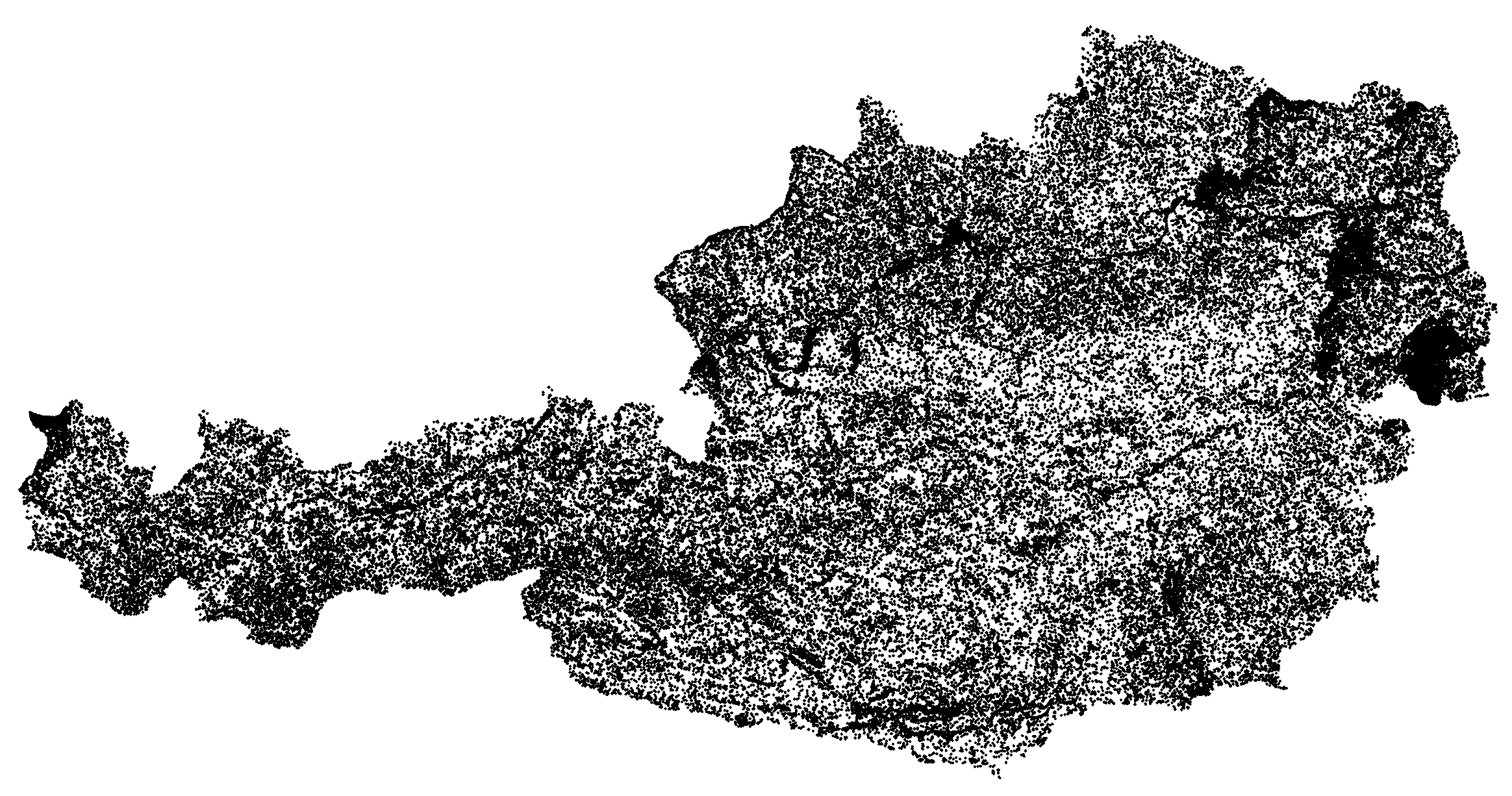
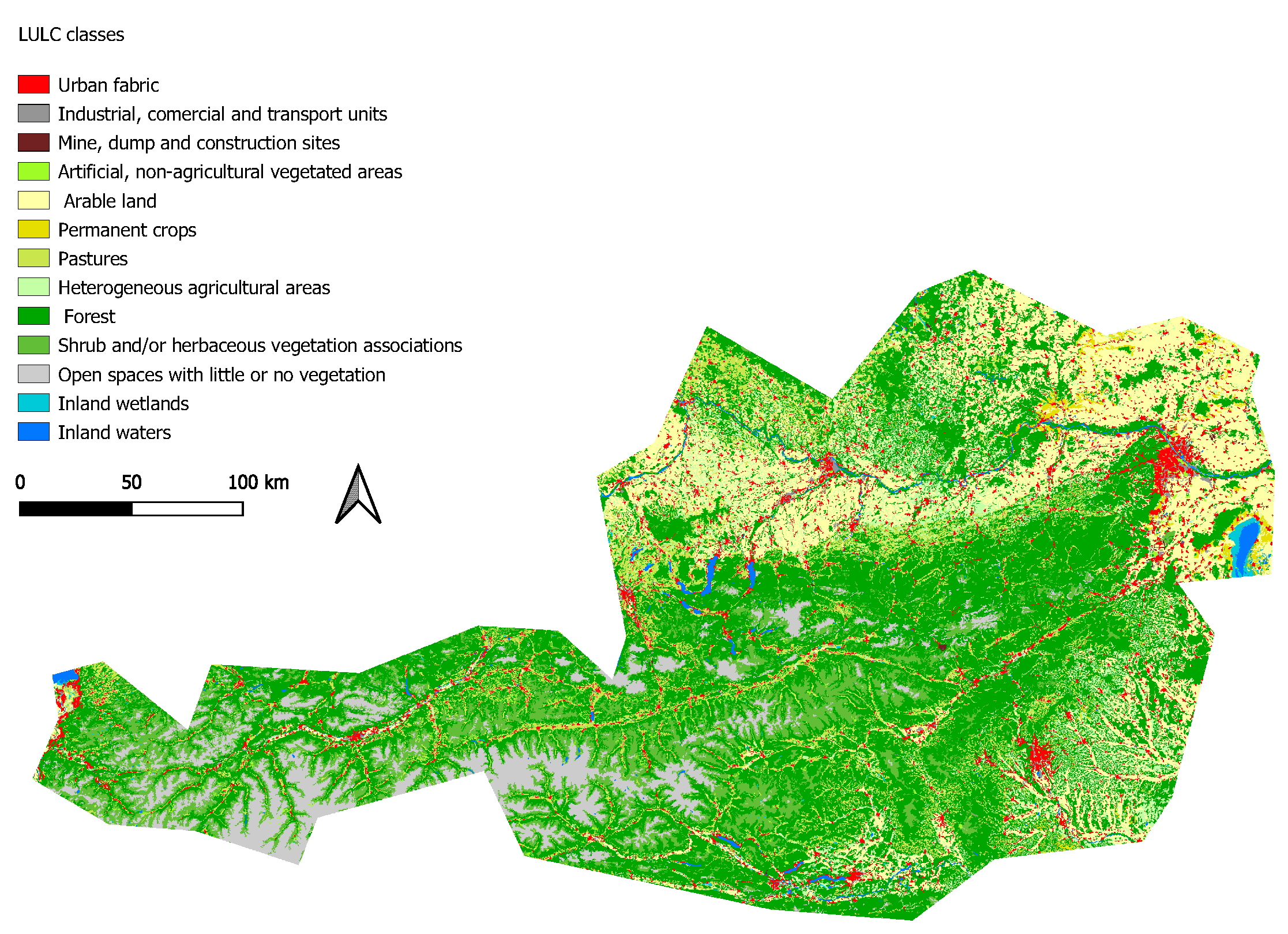
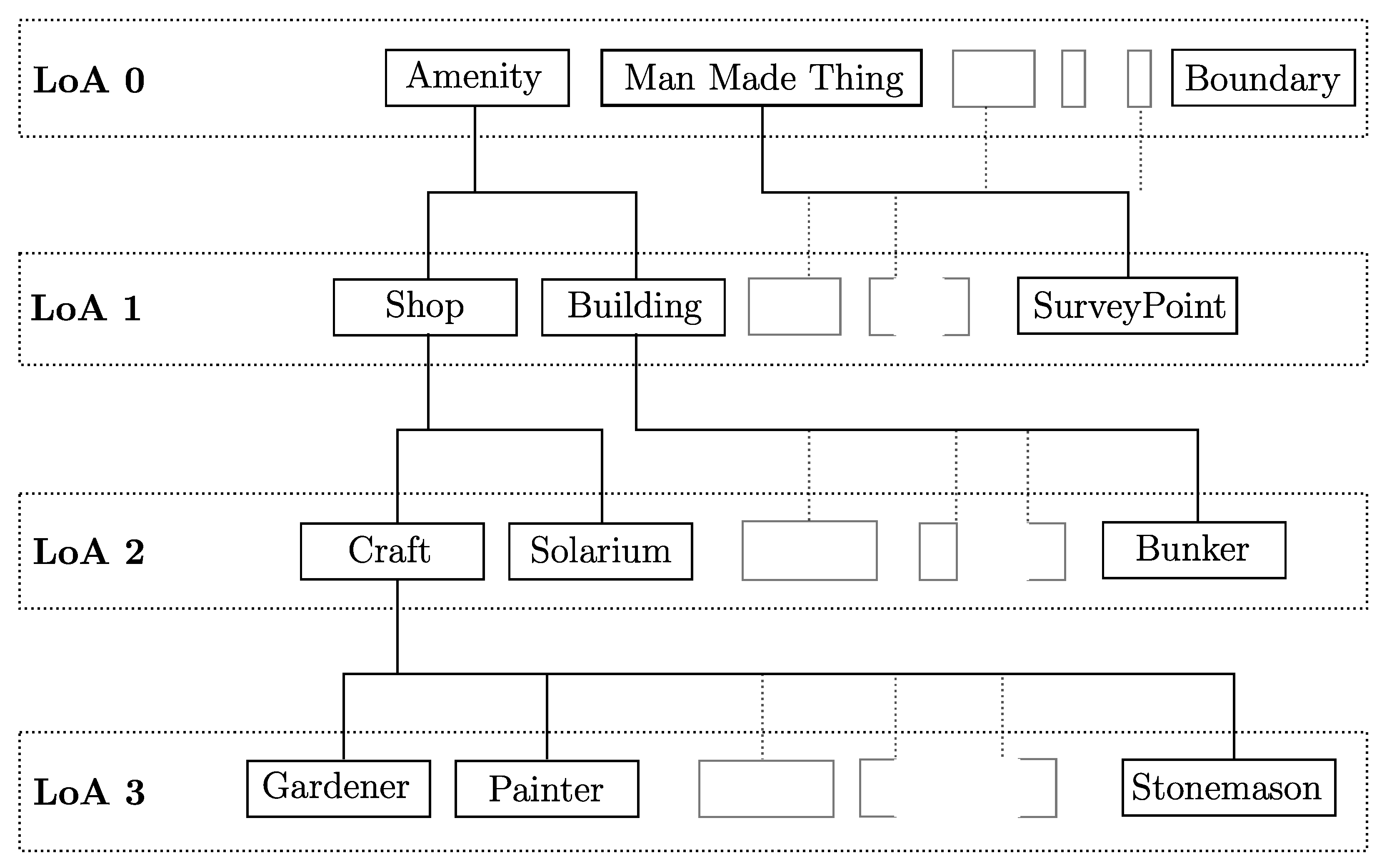
The two datasets were obtained for the entire ROI of this work, which is Austria (the ROI and sample locations are depicted in Figure 2). CORINE Level 2 for the year 2018 was used as ground truth (see Figure 3) as it is a well-studied LULC dataset used by others as ground truth as well [2,30,31,32,33]. The task within both experiments was to predict the LULC classes provided by CORINE. There are 13 different LULC classes within the ROI (see Table 1). A total of 2 of the 15 originally available LULC were not available in the ROI, as Austria is landlocked (LULC classes Marine Waters and Coastal Wetlands are missing). Some 12,000 LULC grid-cells were randomly selected for each LULC class which were then used in Experiment one and Experiment two for training and testing the classification model. Each of these grid-cells (of size 100 m × 100 m) defines the area and ground truth (the LULC class) for a single sample. An equal number of CORINE grid-cells was selected for each LULC class to have a balanced representation of the LULC in the training and testing dataset for subsequent deep learning in our workflow. The geographic distribution of these samples can be seen in Figure 2. For each of these samples, geospatial vector data was extracted around the sample center location. This vector data and its semantics were then ultimately used to predict the LULC class of the corresponding sample. The geospatial vector data was obtained from LinkedGeoData [34], which derives its data from OSM and enhances the object description with an ontology. This enables the description of a single geo-object in terms of multiple Web Ontology Language (OWL) classes which exhibit defined super- and sub-class relationships to each other. For example, a geo-object might be of type PetShop; however, given the ontology, it automatically is also of type Shop and Amenity. This is because the ontology defines PetShop as a subclass of Shop, and Shop as a sub-class of Amenity. Each geo-object is additionally characterized by a geometry which can either be a point (e.g., for the location of a Street sign), a linestring (e.g., for the course of a Street), or a polygon (e.g., for the footprint of a Building).

3.2. Experiment One

Based on these two input datasets Experiment one was carried out. In this experiment the geospatial vector data was encoded using four different approaches: (1) the Geospatial Configuration Matrix (GSCM), (2) the Layered GSCM (LGSCM), (3) the Channel GSCM (CGSCM), (4) and the CUBE Encoding (CUBE). These encodings transform the vector data and its semantic annotations to different numeric feature spaces. For each of the encodings, an optimized Perceiver architecture was searched for. This was accomplished by using a hyperparameter search. Subsequently, the networks were trained and tested using cross-validation folds. This provided us with an accuracy assessment for the comparison of the encodings. The encoding and its corresponding Perceiver network which scored the highest overall accuracy was then used further for Experiment two.

3.2.1. The GSCM Encoding

The GSCM (see Figure 4a), proposed by [4], calculates local statistics for each sample location. Therefore, for each geo-object class (OWL classes such as Restaurant, School, Shop etc.), 9 different statistics were calculated: the standard deviation, the mean as well as the minimum and maximum of all azimuths and distances for the corresponding geo-object class (these are 8 out of the 9 values), as well as the number of geo-objects of this class in the sample area (adding up to 9 values). As there are 1300 different OWL classes, a total of 11,700 features were calculated for each sample (9 × 1300). For calculating the distances and azimuths, the centroids of the geo-objects were used. The default values in case an object class was not present were the same as defined by [4]. For example, 1000.0 (which is the d m a x value) was used for the minimum and maximum distance value in case an OWL class was not present. For the GSCM a hyperparameter has to be set which defines the proximity to the sample location in which geo-objects are considered for the GSCM calculation. This parameter is denoted as d m a x . In this work, we use the recommended value found by [2] for d m a x of 1 km for LULC classification.

3.2.2. The Layered GSCM Encoding

The layered GSCM (LGSCM) is a modification of the GSCM (see Figure 4b). Instead of defining one d m a x value, a series of d m a x values can be defined. These d m a x values define regions around the sample center for which the 11,700 values were computed. For example, if the first d m a x value is 500 m and the second 1 km, the 11,700 descriptive features were calculated for the circle area of 500 m around it, as well as the ring-shaped area which lays 500 m to 1 km away from the sample center. This would result in 11,700 × 2 features for each sample. As such, increasing the number of d m a x threshold values would result in a higher number of input features for the deep neural network. In this work, we used three d m a x values: 333.3 m, 666.6 m and 1 km. Thus, the maximum d m a x value was set to 1 km (same as at the GSCM, to keep it comparable) and equally divided by 3. It was divided equally, to have rings of equal width. Choosing a number higher than 3 resulted in a Perceiver network with unfeasible computational complexity. As such, we chose to use the maximum possible number, which was 3. The feature vector of each sample therefore had the length of 351,003 elements (3 × 11,700 descriptive features). Nevertheless, the number of zones as well as their width can be subject to a separate parameter tuning procedure. However, we leave this for future research.

3.2.3. The Channel GSCM Encoding

The channel GSCM (CGSM) describes each of the 9 descriptive values for each OWL class in a separate input channel (see Figure 4c). Thus, the CGSCM does not represent the input in a vector with a length of 11,700 elements, but a tensor of shape [9,1300], where 1300 is the number of channels, one for each OWL class. As such, the Perceiver network used for this encoding can utilize a channel-wise representation of the input. In addition, for this encoding a d m a x value of 1 km was used.

3.2.4. The CUBE Encoding

The CUBE encoding generates a heatmap for each OWL class (see Figure 4d), stacking them together to a cube-shaped tensor. Each heatmap has an extend of 2000 m × 2000 m to cover a GSCM with radius d m a x = 1000 m. As there are 1300 potential OWL classes, the CUBE has 1300 channels (one for each OWL class). Each heatmap consists of 100 × 100 grid-cells, where each one has an extend of 20 m × 20 m representing the frequency of geo-objects for the corresponding OWL class in this grid area. This resolution was chosen for two reasons: (1) The locations of the geo-objects should be preserved as much as possible. This preservation is increased with a raising resolution, while a reduced resolution can prune this spatial information. Consequently, the highest possible resolution was selected. (2) However, while this resolution may not have a theoretical limit, it has one in practice due to computational limitations. As such, the resolution was chosen based on two objectives: Maintaining the highest possible resolution while also maintaining the computational workload feasible. This was the case for 20 m, which we found to be the optimal solution regarding both objectives. The aim of using heatmaps is to allow the Perceiver network to learn based on the spatial distributions directly, instead of statistics which aggregate information on the spatial distribution of the geo-objects (which is the case for the other encodings).
A separate deep learning pipeline was created for each encoding type (see Figure 1). The same sequence of steps was performed in each pipeline: (1) Split the (already encoded) data into 5 folds. This was completed to perform a 5-fold cross validation at a later stage. (2) Based on the first fold, search for optimal hyperparameters for the Perceiver network. This was performed using Optuna [35] which is a library for hyperparameter search and agnostic to the model type. (3) Train and test the Perceiver network based on the optimized hyperparameters in a 5-fold cross-validation manner.

3.2.5. The Perceiver Model

The Perceiver network [6] aims at optimizing the runtime complexity of the Transformer network [5] by introducing a bottleneck in its architecture. In addition, it is a general-purpose network as it can handle different data modalities, such as audio or 3D-pointclouds due to its flexible Fourier-based positional encoding. The Fourier-based encoding applies attention at different frequencies for different data granularities. There are multiple potential ANN architectures (e.g., MLP, CNN, RNN, etc.) which could be chosen in practice to perform the LULC classification in this work. However, there are two requirements which must be fulfilled by the potential architecture, and the Perceiver fulfills them both: First, the same network type had to be used for all encodings to aim at a fair comparison among them. However, since the shapes of the encodings were different, a network architecture was required which supports this variation. For example, while [2,4] used a multilayer perceptron (MLP) for training a GSCM, a MLP would not fit this requirement for the other encodings proposed in this work. This is because the shape of the encodings used here can exceed one-dimensional feature vectors (such as the CUBE encoding). Second, the ANN was not allowed to assume that nearby features are correlated. This is the case for convolutional neural networks, which make such an assumption by training weight matrices patch-wise. The Perceiver meets both requirements as it can forward tensors of different dimensions (first requirement), and it uses attention mechanism to detect the relationship of different features (second requirement). We chose the Perceiver network as it fulfills both requirements.

3.2.6. Hyperparameter Optimization

For hyperparameter optimization, the Tree-structured Parzen Estimator (TPE) [36] was used, as this is the recommended default setting. The TPE searches for optimal hyperparameters in the search space in an iterative manner. Moreover, it therefore adjusts the hyperparameters based on previous hyperparameter configurations and their associated accuracy scores (we used the overall accuracy for that). A total of 30 trials for each encoding were performed.
The Perceiver hyperparameters which were subject to this optimization procedure can be seen in Table 2. Please note that for each of the four deep learning pipelines in Experiment one, the hyperparameter search spaces were the same.

3.2.7. Training and Testing the Model

This results in four different Perceiver networks which all have optimized hyperparameter with regards to the input encoding. Each of the four models was then evaluated in a 5-fold cross-validation manner. For each fold, 5 different metrics were calculated to assess the model performance for the corresponding fold. Then, based on the 5 folds, an average value was computed for each of the 5 metrics. We employed the following 5 metrics: (1) overall accuracy; (2) kappa value; (3) recall; (4) precision and (5) confusion matrix. These were defined as:
Overall accuracy:
overall accuracy = number of all correct predictions number of all wrong predictions
Kappa [37]:
κ = p 0 p c 1 p c
p 0 is the proportion of correct predictions and p c the expected proportion of predictions due to chance [37].
Recall and precision:
recall = true positive true positive + false positive
precision = true positive true positive + false positive
Based on these metrics, the best performing model and the respective encoding were used for Experiment two.

3.3. Experiment Two

In Experiment two, the aim was to explore the influence a varying level of knowledge on the semantics has on the LULC classification. For example, how does the model performance change once there are only 50 OWL classes available describing geo-object types, versus, when all 1300 OWL classes are available? The OWL ontology describes these classes, such as BeautyShop or Amenity, respectively (see Figure 5 for examples and visualization). These OWL classes exhibit sub- and super-class relationships to each other. Please note, the OWL classes were not defined by us, but by LinkedGeoData [34]. We denote the level of knowledge, which describes different granularities of semantics, as the the level of abstraction (LoA). The LoA descibes the levels in the lattice-like structured OWL ontology, and we define it as the maximum number of super-classes an OWL class has. The top layer of this OWL lattice structure contains the most abstract geo-object types (i.e., OWL-classes such as Amenity or Boundary). We denote this layer LoA 0 as it is the first layer. The least abstract geo-objects (e.g., Gardener, Beekeeper, etc. in Figure 5) are in the last (the fourth) layer which we denote LoA 3. The LoAs between are denoted LoA 1 and LoA 2. LoA 1 contains more abstract classes than LoA 2. Thus, there are four levels of abstraction. In Experiment two, these four LoAs were used to parametrize the detail of knowledge on geo-objects. They were pruned one by one and the LULC was then re-run based on the pruned dataset (using the model and encoding from Experiment one which scored the highest classification accuracy). Three pruned datasets were created: (I) OWL classes of LoA 3 were pruned (denoted L.0–2); (II) OWL classes of LoA 3 and 2 were pruned (denoted L.0–1); (III) OWL classes of LoA 3 to 1 were pruned (denoted L.0). Not all geo-objects belong to LoA 3, 2 or 1 (and therefore to all other LoAs); however, they at least belong to LoA0. A geo-object may, for example, be of type Shop and an Amenity only. As such, this pruning strategy ensured that no geo-object was lost in a dataset, but only OWL-class information was removed (due to its super- and sub-class relationship). For example, a PetShop is always also a Shop and Amenity. Therefore, no information loss (or gain) was due to missing geographic information. Once the model was re-run on each of the pruned datasets, their classification performance was measured with the same metrics as in Experiment one.

4. Results and Analysis

4.1. Experiment One

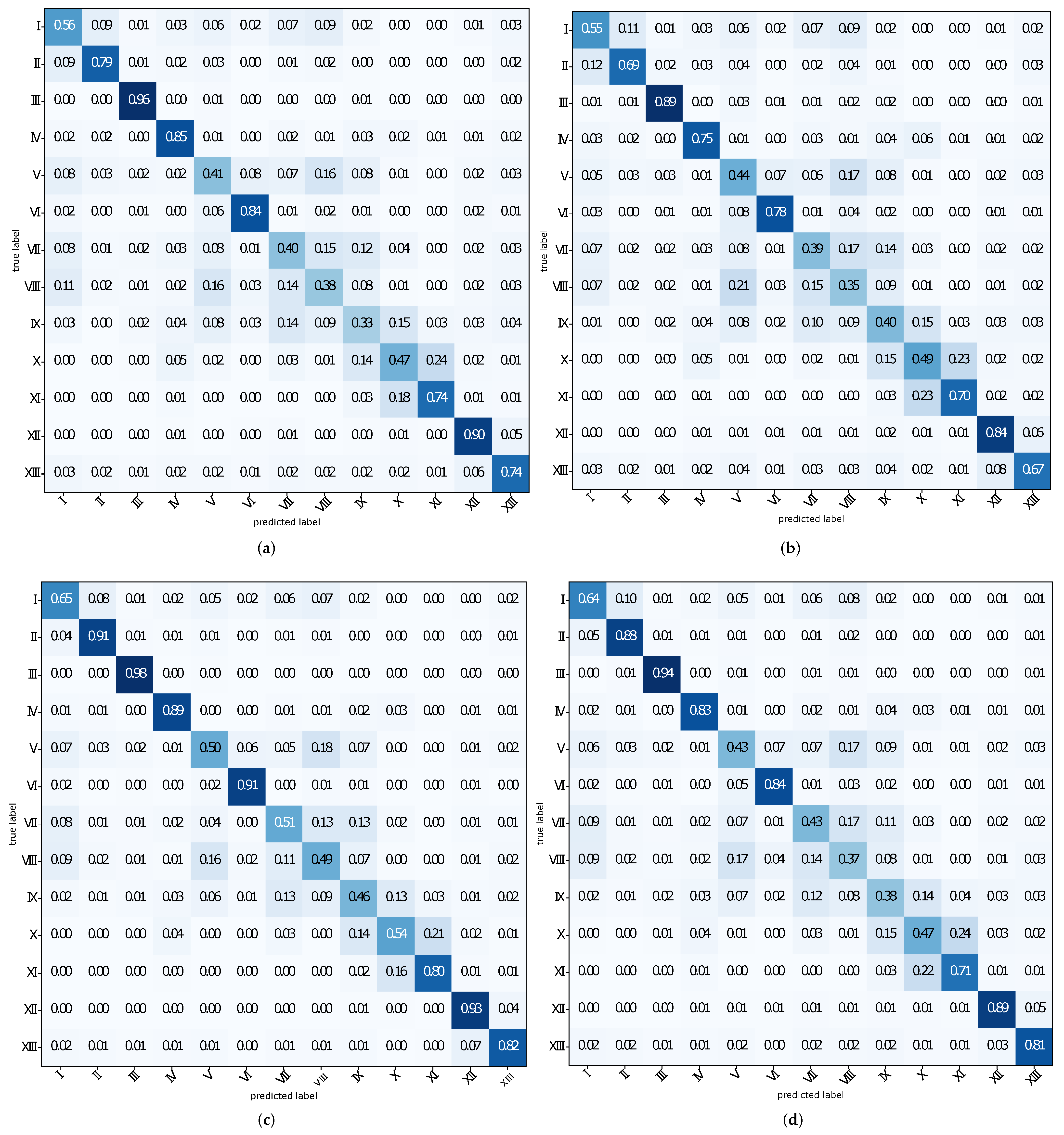
The overall accuracies and kappa coefficients scored with each encoding in Experiment one can be seen in Table 3. The highest overall accuracy and kappa coefficient were scored for the same encoding, the CGSCM. The second highest overall accuracy was scored using the CUBE with 66%. The third and fourth highest overall performance was scored by the GSCM and LGSCM, respectively. Consequently, forwarding the local statistics channel-wise to the Perceiver provides superior results in Experiment one. A similar behavior is seen for recall and precision (see Table 4): The highest recall and precision were scored for the CGSCM. Concerning the other encodings, the CUBE encoding scored the highest recall for LULC classes I (Urban Fabric), IV (Artificial, non-agricultural vegetated areas), V (Arable land), VI (Permanent crops), IX Forest, XII Inland wetlands and XIII Inland waters. In contrast, the recall for the GSCM exceeds for LULC classes II (Industrial, commercial and transport units), III (Mine, dump and construction sites), X (Scrub and/or herbaceous vegetation associations) and XI (Open spaces with little or no vegetation). The LGSCM has an inferior recall and precision compared to the other encodings. Furthermore, the recall for the CUBE encodings is higher than for the GSCM for LULC classes I (Urban Fabric), II (Industrial, commercial and transport units), V (Arable land), VII (Pastures), IX (Forest) and XIII (Inland waters). The confusion matrices (see Figure 6a–d) also show that the CGSCM confuses the LULC classes the least with each other. However, next to the individual encoding performances another pattern can be detected: The same LULC classes were confused most strongly among all encodings, however, with different magnitude depending on the encoding. For example, LULC classes VII (Pastures), VIII (Heterogeneous agricultural areas) and IX (Forest) are among the most confused for all encodings. The same is true for LULC classes XI (Open spaces with little or no vegetation) and X (Scrub and/or herbaceous vegetation associations). The hyperparameters which were determined using OPTUNA can be seen in Table 5. The optimizer used in this work is LAMB [38] as it was the recommended optimizer by [6].

4.2. Experiment Two

Table 6 shows the overall accuracies as well as kappa coefficients which were scored with different LoAs. It can be seen that the varying availability of semantics has an impact on the LULC classification performance. Specifically, the highest overall accuracy and kappa coefficient were scored when using all the available LoAs (L.0–3). The biggest gain in classification accuracy was obtained once LoA 1 is used too, i.e., when moving from L.0 to L.0–1. Considering the recall and precision (see Table 7), it can be seen that using all available LoAs yields the highest scores. Furthermore, some LULC classes benefit more than others from using semantics. For example, LULC classes I to IV have a higher precision and recall than LULC class V. However, all recall and precision scores increase when increasing the LoA too. Another observation can be made when using L.0–3. While the overall performance gain is not as high as for moving from L.0 to L.0–1 (see Table 6), two LULC classes change in recall more than others (see Table 6): LULC XI increasing from0.74 to0.80 and LULC class X dropping from0.60 to0.54. The same observation is not made for the precision. Here, it is important to note that the difference between LoA 2 and LoA3 is a set of very specific OWL classes which relate to Crafts such as Painter, Beekepper or Gardener (see Figure 5 for further examples).
The confusion matrices (see Figure 7a–d) confirm prior observations of the overall classification performance. For example, the confusions among the LULC classes also decrease here the most when increasing LoA 0 to LoA 0 and 1 (see Figure 7a,b), respectively). Increasing to LoA 2 and LoA 3 (see Figure 7c,d), respectively) but with a lower magnitude also confuses. Here, some minor changes in confusions with LULC classes X, XI and class I can be observed when including LoA 3.

5. Discussion

5.1. Experiment One

Experiment one revealed that the encoding type influences the LULC classification performance. The CGSCM scored the highest classification performance, which passes the GSCM to the Perceiver channel-wise (i.e., the CGSCM). This suggests that a feature space which allows us to access the same descriptive values (stored in one channel) of the GSCM but for different OWL classes provides an advantage when modeling LULC. As such, not only the way how the geo-objects are encoded matters, but also how this representation is embedded in a feature space. In contrast, the CUBE encoding aims at maintaining the spatial distributions of the different geo-objects (via the heatmap). Based on the corresponding overall accuracy and kappa coefficient, it can be seen that this did not provide an advantage. However, another possible reason for this can be that the Perceiver network was unable to facilitate this information more effectively. Next to the overall performance, the recall, precision as well as confusions revealed that a series of LULC classes were captured more precisely than others when using semantics, regardless of how the geography is encoded. Consequently, encoding geo-objects by using descriptive statistics (GSCM) or heatmaps only influenced the overall classification performance and not the relative classification performances of single LULC classes. This suggests that the encoding of the geography influences the overall performance rather than the performance for specific LULC classes. Nevertheless, we also observed limitations of a computational nature within Experiment one. Encoding the geospatial vector data can be a computationally demanding task. This is because for each sample location, all vector data has to be queried within the d m a x perimeter and then converted into the right encoding scheme. We addressed this problem in practice by implementing the encoding in a multi-threaded manner. Another limitation is caused by the Perceiver network, as it can be computationally challenging to train and test. The reason for this is the computationally demanding attention mechanism and an increased number of weights which need to be trained (depending on the hyperparameters, 80 million to 300 million weights in our case). We tackled this problem by using eight A100 GPU (from Nvidia®) in parallel to train and test the networks.

5.2. Experiment Two

Experiment two showed that semantics can influence both the overall accuracy as well as the relative classification performance of single LULC classes. Having more information (parameterized via the LoAs) on the geo-object types can thus help increase the LULC classification performance overall and for single LULC classes. Using all available LoAs yielded the highest classification performance which suggests that more information on the geo-object types yields a higher classification performance. However, this increase of performance seemed to converge. Thus, while semantics allows us to discriminate LULC, the discrimination power depends on the granularity of the semantics.
Moreover, including specific OWL classes changed the information on specific LULC classes. This was seen in the case of adding LoA3, which contained OWL classes such as Plumber, Gardener, Beekeeper, etc. which are all sub-classes of a single OWL class Craft. The recall changed mostly for LULC XI (increasing from 0.74 to 0.80) and LULC X (dropping from 0.60 to 0.54). A potential explanation for this is that Services/Crafts are more likely to be found where they can be offered to customers. However, while they may belong to different LULC classes (e.g., a Beekeeper at LULC class Forests, a Plumber at Urban fabric) finding such services in the alpine area of Austria is unlikely. Alpine area is of LULC type Open spaces with little or no vegetation (LULC class XI) and covers a significant part of the ROI. Thus, the absence of any Craft potential has helped to recall that a certain area is not of LULC class Open spaces with little or no vegetation. The same assumption, however, can be made for Inland wetlands and Inland waters too, which are unlikely to be inhabited by mankind. Nevertheless, when they are close to urban areas (e.g., a river) or essential to tourism (e.g., water sport), this assumption does not hold.

6. Conclusions and Future Research

In this work, different geographic encoding schemes and semantic granularities (LoA) were used to classify LULC. Therefore, two experiments were carried out which resulted in three findings: (1) Semantics can be used to classify LULC, confirming prior research [2]. (2) The way the geography of the corresponding geo-objects is encoded influences the overall LULC classification performance. In particular, the CGSCM was found to be the encoding which yielded the highest LULC classification performance, followed by the CUBE encoding. (3) The granularity of the semantics (LoA) influences the overall classification performance and discrimination power for single LULC classes. The granularity of the semantics was represented by the LoA. Our findings suggest that the prediction performance increases once more semantics are available. Nevertheless, future research can focus on other ways for pruning OWL ontology than using the LoA. For example, OWL classes which are likely to co-locate with others could be pruned. This can potentially help reduce the computational cost of using all 1300 OWL classes of the ontology while preserving the discriminative power. Another potential research target in this realm is the creation of a case specific ontology which increases the classification performance further. In this work, a Perceiver network was employed for deep learning. While this network was capable of training based on different modalities, other ANN could be tested as well in the future. Prior work has performed image fusion with semantics [2]. The CUBE encoding presented in this work is an ideal candidate for such a fusion due to its heatmap representation; additional image channels could be stacked to it. This data fusion is another potential research direction. While we employed encodings in this work which focus on different geographic characteristics, future research could focus on learnable embeddings for geographic information with semantic annotations. This might lead to higher overall classification performances but may also allow it to fuse with other data sources. The irregularity and heterogeneity of geospatial vector data with semantics makes this a challenging but also fruitful research direction. Moreover, the data which were used here are volunteered geographic information [39] collected via OSM; however, other data sources could be considered, for example from augmented reality recordings [40] or street level information [7], which could provide enhanced semantics. In addition, while this work focused on a quantitative analysis of the results, future work can consider qualitative assessment methods such as geovisualization of the results.

Author Contributions

Conceptualization, M.M.C.; Data curation, M.M.C.; Formal analysis, M.M.C.; Investigation, M.M.C.; Methodology, M.M.C. and I.G.; Project administration, I.G.; Software, M.M.C.; Supervision, I.G.; Visualization, M.M.C.; Writing—original draft, M.M.C.; Writing—review & editing, M.M.C. and I.G. All authors have read and agreed to the published version of the manuscript.

Funding

Open Access Funding by TU Wien.

Data Availability Statement

Data available on request due to restrictions, e.g., privacy or ethical.

Conflicts of Interest

The authors declare no conflict of interest.

References

  1. Fisher, P. The pixel: A snare and a delusion. Int. J. Remote Sens. 1997, 18, 679–685. [Google Scholar] [CrossRef]
  2. Mc Cutchan, M.; Comber, A.J.; Giannopoulos, I.; Canestrini, M. Semantic Boosting: Enhancing Deep Learning Based LULC Classification. Remote Sens. 2021, 13, 3197. [Google Scholar] [CrossRef]
  3. Mc Cutchan, M.; Giannopoulos, I. Geospatial Semantics for Spatial Prediction. In Leibniz International Proceedings in Informatics (LIPIcs); Winter, S., Griffin, A., Sester, M., Eds.; Schloss Dagstuhl–Leibniz-Zentrum fuer Informatik: Dagstuhl, Germany, 2018; Volume 114, pp. 45:1–45:6. [Google Scholar] [CrossRef]
  4. Mc Cutchan, M.; Özdal Oktay, S.; Giannopoulos, I. Semantic-based urban growth prediction. Trans. GIS 2020, 24, 1482–1503. [Google Scholar] [CrossRef]
  5. Vaswani, A.; Shazeer, N.; Parmar, N.; Uszkoreit, J.; Jones, L.; Gomez, A.N.; Kaiser, Ł.; Polosukhin, I. Attention is all you need. Adv. Neural Inf. Process. Syst. 2017, 30, 5998–6008. [Google Scholar]
  6. Jaegle, A.; Gimeno, F.; Brock, A.; Zisserman, A.; Vinyals, O.; Carreira, J. Perceiver: General Perception with Iterative Attention. arXiv 2021, arXiv:2103.03206. [Google Scholar]
  7. Ertler, C.; Mislej, J.; Ollmann, T.; Porzi, L.; Kuang, Y. Traffic Sign Detection and Classification around the World. In Proceedings of the European Conference on Computer Vision (ECCV), Glasgow, UK, 23–28 August 2020. [Google Scholar]
  8. Veer, R.V.; Bloem, P.; Folmer, E. Deep learning for classification tasks on geospatial vector polygons. arXiv 2018, arXiv:1806.03857. [Google Scholar]
  9. Yan, B.; Janowicz, K.; Mai, G.; Gao, S. From ITDL to Place2Vec: Reasoning About Place Type Similarity and Relatedness by Learning Embeddings From Augmented Spatial Contexts. In Proceedings of the 25th ACM SIGSPATIAL International Conference on Advances in Geographic Information Systems (SIGSPATIAL ’17), Redondo Beach, CA, USA, 7–10 November 2017; Association for Computing Machinery: New York, NY, USA, 2017. [Google Scholar] [CrossRef]
  10. Zhang, Y.; Li, Q.; Tu, W.; Mai, K.; Yao, Y.; Chen, Y. Functional urban land use recognition integrating multi-source geospatial data and cross-correlations. Comput. Environ. Urban Syst. 2019, 78, 101374. [Google Scholar] [CrossRef]
  11. Mikolov, T.; Sutskever, I.; Chen, K.; Corrado, G.; Dean, J. Distributed Representations of Words and Phrases and their Compositionality. Adv. Neural Inf. Process. Syst. 2013, 26, 3111–3119. [Google Scholar] [CrossRef]
  12. Grekousis, G.; Mountrakis, G.; Kavouras, M. An overview of 21 global and 43 regional land-cover mapping products. Int. J. Remote Sens. 2015, 36, 5309–5335. [Google Scholar] [CrossRef]
  13. Thanh Noi, P.; Kappas, M. Comparison of Random Forest, k-Nearest Neighbor, and Support Vector Machine Classifiers for Land Cover Classification Using Sentinel-2 Imagery. Sensors 2017, 18, 18. [Google Scholar] [CrossRef]
  14. Mishra, V.N.; Prasad, R.; Kumar, P.; Gupta, D.K.; Dikshit, P.K.S.; Dwivedi, S.B.; Ohri, A. Evaluating the effects of spatial resolution on land use and land cover classification accuracy. In Proceedings of the 2015 International Conference on Microwave, Optical and Communication Engineering (ICMOCE), Bhubaneswar, India, 18–20 December 2015; pp. 208–211. [Google Scholar]
  15. Ma, L.; Li, M.; Ma, X.; Cheng, L.; Du, P.; Liu, Y. A review of supervised object-based land-cover image classification. ISPRS J. Photogramm. Remote Sens. 2017, 130, 277–293. [Google Scholar] [CrossRef]
  16. Comber, A.J.; Wadsworth, R.A.; Fisher, P.F. Using semantics to clarify the conceptual confusion between land cover and land use: The example of ‘forest’. J. Land Use Sci. 2008, 3, 185–198. [Google Scholar] [CrossRef]
  17. Foley, J.A. Global Consequences of Land Use. Science 2005, 309, 570–574. [Google Scholar] [CrossRef] [PubMed]
  18. Pielke, R.A. Land Use and Climate Change. Science 2005, 310, 1625–1626. [Google Scholar] [CrossRef]
  19. Pielke, R.A., Sr.; Pitman, A.; Niyogi, D.; Mahmood, R.; McAlpine, C.; Hossain, F.; Goldewijk, K.K.; Nair, U.; Betts, R.; Fall, S.; et al. Land use/land cover changes and climate: Modeling analysis and observational evidence. WIREs Clim. Chang. 2011, 2, 828–850. [Google Scholar] [CrossRef]
  20. Li, Z.; White, J.C.; Wulder, M.A.; Hermosilla, T.; Davidson, A.M.; Comber, A.J. Land cover harmonization using Latent Dirichlet Allocation. Int. J. Geogr. Inf. Sci. 2020, 35, 348–374. [Google Scholar] [CrossRef]
  21. Polasky, S.; Nelson, E.; Pennington, D.; Johnson, K.A. The Impact of Land-Use Change on Ecosystem Services, Biodiversity and Returns to Landowners: A Case Study in the State of Minnesota. Environ. Resour. Econ. 2011, 48, 219–242. [Google Scholar] [CrossRef]
  22. De Chazal, J.; Rounsevell, M.D. Land-use and climate change within assessments of biodiversity change: A review. Glob. Environ. Chang. 2009, 19, 306–315. [Google Scholar] [CrossRef]
  23. Tayebi, M.; Fim Rosas, J.T.; Mendes, W.D.S.; Poppiel, R.R.; Ostovari, Y.; Ruiz, L.F.C.; dos Santos, N.V.; Cerri, C.E.P.; Silva, S.H.G.; Curi, N.; et al. Drivers of Organic Carbon Stocks in Different LULC History and along Soil Depth for a 30 Years Image Time Series. Remote Sens. 2021, 13, 2223. [Google Scholar] [CrossRef]
  24. Metzger, M.; Rounsevell, M.; Acosta-Michlik, L.; Leemans, R.; Schröter, D. The vulnerability of ecosystem services to land use change. Agric. Ecosyst. Environ. 2006, 114, 69–85. [Google Scholar] [CrossRef]
  25. Fu, P.; Weng, Q. A time series analysis of urbanization induced land use and land cover change and its impact on land surface temperature with Landsat imagery. Remote Sens. Environ. 2016, 175, 205–214. [Google Scholar] [CrossRef]
  26. Debbage, N.; Shepherd, J.M. The urban heat island effect and city contiguity. Comput. Environ. Urban Syst. 2015, 54, 181–194. [Google Scholar] [CrossRef]
  27. Schultz, M.; Voss, J.; Auer, M.; Carter, S.; Zipf, A. Open land cover from OpenStreetMap and remote sensing. Int. J. Appl. Earth Obs. Geoinf. 2017, 63, 206–213. [Google Scholar] [CrossRef]
  28. Mai, G.; Janowicz, K.; Yan, B.; Zhu, R.; Cai, L.; Lao, N. Multi-Scale Representation Learning for Spatial Feature Distributions using Grid Cells. arXiv 2020, arXiv:2003.00824. [Google Scholar]
  29. Yan, X.; Ai, T.; Yang, M.; Tong, X. Graph convolutional autoencoder model for the shape coding and cognition of buildings in maps. Int. J. Geogr. Inf. Sci. 2021, 35, 490–512. [Google Scholar] [CrossRef]
  30. Bengana, N.; Heikkilä, J. Improving Land Cover Segmentation Across Satellites Using Domain Adaptation. IEEE J. Sel. Top. Appl. Earth Obs. Remote Sens. 2021, 14, 1399–1410. [Google Scholar] [CrossRef]
  31. Antropov, O.; Rauste, Y.; Šćepanović, S.; Ignatenko, V.; Lönnqvist, A.; Praks, J. Classification of Wide-Area SAR Mosaics: Deep Learning Approach for Corine Based Mapping of Finland Using Multitemporal Sentinel-1 Data. In Proceedings of the IGARSS 2020—2020 IEEE International Geoscience and Remote Sensing Symposium, Waikoloa, HI, USA, 26 September–2 October 2020; pp. 4283–4286. [Google Scholar] [CrossRef]
  32. Balado, J.; Arias, P.; Díaz-Vilariño, L.; González-deSantos, L.M. Automatic CORINE land cover classification from airborne LIDAR data. Procedia Comput. Sci. 2018, 126, 186–194. [Google Scholar] [CrossRef]
  33. Balzter, H.; Cole, B.; Thiel, C.; Schmullius, C. Mapping CORINE Land Cover from Sentinel-1A SAR and SRTM Digital Elevation Model Data using Random Forests. Remote Sens. 2015, 7, 14876–14898. [Google Scholar] [CrossRef]
  34. Stadler, C.; Lehmann, J.; Höffner, K.; Auer, S. LinkedGeoData: A Core for a Web of Spatial Open Data. Semant. Web J. 2012, 3, 333–354. [Google Scholar] [CrossRef]
  35. Akiba, T.; Sano, S.; Yanase, T.; Ohta, T.; Koyama, M. Optuna: A Next-generation Hyperparameter Optimization Framework. In Proceedings of the 25rd ACM SIGKDD International Conference on Knowledge Discovery and Data Mining, Anchorage, AK, USA, 4–8 August 2019. [Google Scholar]
  36. Bergstra, J.; Bardenet, R.; Bengio, Y.; Kégl, B. Algorithms for Hyper-Parameter Optimization. In Advances in Neural Information Processing Systems; Shawe-Taylor, J., Zemel, R., Bartlett, P., Pereira, F., Weinberger, K.Q., Eds.; Curran Associates, Inc.: Red Hook, NY, USA, 2011; Volume 24. [Google Scholar]
  37. Cohen, J. A Coefficient of Agreement for Nominal Scales. Educ. Psychol. Meas. 1960, 20, 37–46. [Google Scholar] [CrossRef]
  38. You, Y.; Li, J.; Hseu, J.; Song, X.; Demmel, J.; Hsieh, C. Reducing BERT Pre-Training Time from 3 Days to 76 Minutes. arXiv 2019, arXiv:1904.00962. [Google Scholar]
  39. Goodchild, M. Citizens as Sensors: The World of Volunteered Geography. GeoJournal 2007, 69, 211–221. [Google Scholar] [CrossRef]
  40. Gokl, L.; Mc Cutchan, M.; Mazurkiewicz, B.; Fogliaroni, P.; Giannopoulos, I.; Fogliaroni, P.; Mazurkiewicz, B.; Kattenbeck, M.; Giannopoulos, I.; Fogliaroni, P.; et al. Towards urban environment familiarity prediction. Adv. Cartogr. Gisci. ICA 2018, 62, 26. [Google Scholar] [CrossRef]
Figure 1. An overview of the workflow. CORINE LULC Level 2 data and geospatial vector data are used as input. Experiment one was carried out before Experiment two, and Experiment two was based on the outcome of Experiment one. In particular, in Experiment one, four different encodings were used to transform the geospatial vector data and its semantic annotations for predicting the LULC ground truth (given from CORINE). For each encoding, a separate processing pipeline for hyperparameter search and model training/testing (with accuracy assessment) was created. After Experiment one was finished, Experiment two was carried out. Experiment two used the best performing encoding (determined in Experiment one), however with different semantic granularities (i.e., LoA). Please note that the data with LoA 3 in Experiment two is the same data as used in Experiment one, as it uses all the available semantics (OWL classes).
Remotesensing 14 02812 g001
Figure 2. The 12,000 samples were randomly selected as ground truth for each LULC class to train and test the deep learning model (Perceiver network). These sample locations are illustrated in this map as black dots.
Remotesensing 14 02812 g002
Figure 3. The CORINE level 2 data which was used as ground truth over Austria.
Remotesensing 14 02812 g003
Figure 4. The four encodings presented in this work. All of them quantify the geospatial vector data differently: (a) shows the GSCM which was introduced by [4] (image source: [4]); (b) shows the layered GSCM (LGSCM) which computes descriptive statistics for different ring regions. For each ring region descriptive values are computed for each OWL class; (c) shows the channel GSCM (CGSCM) which provides a channel-wise representation of the descriptive values. In (ac) the different geo-object types (OWL classes) are indicated by different shapes; (d) shows the CUBE encoding which represents the geographic distribution of each geo-object type as a heatmap. In this visualization, only three of multiple heatmaps are shown. Each heatmap represents the geospatial distribution of a specific OWL class. Here, deep blue grid-cells denote a higher number of geo-objects, whereas the color gradient toward white represents a decreasing number of geo-objects.
Remotesensing 14 02812 g004
Figure 5. Different examples of OWL classes and to which level of abstractions (LoA) they can belong. The OWL classes exhibit a super- and sub- class relationship to each other. For example, Solarium is a sub-class of Shop which is a sub-class of Amenity. A geo-object which is of type Solarium automatically is of type Shop and Amenity too. This figure illustrates the hierarchical lattice structure of the OWL ontology. In Experiment two, specific LoAs were used to find out how important it is for LULC classification to have more detailed knowledge about geo-objects.
Remotesensing 14 02812 g005
Figure 6. The confusion matrices of the four encoding in Experiment one: (a) GSCM; (b) LGSCM; (c) GSCM; (d) CUBE. Please note that in Experiment one all available OWL classes (all LoAs) were used. The horizontal and vertical axis indicates predicted vs.true labels, respectively.
Remotesensing 14 02812 g006
Figure 7. The confusion matrices for classification using different LoAs: (a) for using LoA 0 only. As such, here only the most basic OWL-classes were used; (b) for using LoA 0 and 1; (c) for using LoA 0 to 2; (d) for using LoA 0 to 3 (all OWL classes).
Remotesensing 14 02812 g007
Table 1. The 13 different LULC available in the ROI (Austria). A total of 2 of the original 15 CORINE LULC Level 2 classes were not available as the ROI (Austria) is land-locked. These were Coastal wetlands and Marine waters.
CodeCLC Level 2 LULC Class
IUrban fabric
IIIndustrial, commercial and transport units
IIIMine, dump and construction sites
IVArtificial, non-agricultural vegetated areas
VArable land
VIPermanent crops
VIIPastures
VIIIHeterogeneous agricultural areas
IXForest
XScrub and/or herbaceous vegetation associations
XIOpen spaces with little or no vegetation
XIIInland wetlands
XIIIInland waters
Table 2. Hyperparameter of the Perceiver networks and their search spaces. For all encodings, the same search spaces were used. Please note, continuous search spaces are denoted in square brackets, whereas (discrete) sets are denoted in curly brackets.
Hyperparameter [6]Seach SpaceDescription
Learning rate [ 1 × 10 4 , 1 × 10 4 ] Learning rate
of the LAMB
optimizer
Dropout [ 0.30 , 0.60 ] Dropout for attention
and fully connected
layers
Depth { 6 , 8 , 10 } Number of iteratively
applied Perceiver
blocks
Number of latents { 128 , 256 , 384 , 512 } Number of
centroids
in latent space
Dimension of latents { 128 , 256 , 384 , 512 } Dimension of
latent space
Number of cross-heads { 1 , 2 , 3 , 4 } Number of heads
for cross-attention
Number of latent-heads { 2 , 4 } Number of heads
for latent-attention
Dimension of cross-heads { 128 , 256 , 384 , 512 } Dimension of
each cross-head
Dimension of latent-heads { 128 , 256 , 384 , 512 } Dimension of
each latent-head
Number of self-attention blocks { 1 , 2 , 3 , 4 } Number of self-attention
blocks used
Number of frequency bands { 7 , 8 , 9 , 10 , 11 , 12 , 13 , 14 , 15 } Bands used
for Fourier
positional encoding
Maximum frequency [ 7 , 16 ] Maxium frequency
for Fourier
positional encoding
Table 3. Overall accuracy and kappa coefficients scored for the encodings used in Experiment one.
GSCMLGSCMCGSCMCUBE
OA64.47%61.01%72.31%66.10%
Kappa0.580.540.690.57
Table 4. Recall and Precision for each encoding in Experiment one. The blue color value indicates the magnitude of the values.
PrecisionRecall
GSCMLGSCMCGSCMCUBEGSCMLGSCMCGSCMCUBE
I0.540.580.650.620.560.550.650.64
II0.800.750.840.790.790.690.900.88
III0.900.850.920.890.960.890.980.94
IV0.770.760.870.820.850.750.890.83
V0.440.400.570.480.410.440.500.43
VI0.810.810.880.820.840.780.910.84
VII0.440.420.560.480.400.390.510.43
VIII0.390.340.490.390.380.350.490.37
IX0.380.380.480.410.330.400.460.38
X0.530.480.600.510.470.490.540.47
XI0.700.710.750.690.740.700.800.71
XII0.810.780.850.830.900.840.930.89
XIII0.700.690.840.770.740.670.820.81
Table 5. Hyperparameters obtained using Optuna [35] for the Perceiver networks of each encoding. The LAMB [38] optimizer was used here.
HyperparameterGSCMLGSCMCUBECGSCM
Learning rate0.0002820.0001780.0025580.000242
Dropout0.35960.49360.41230.3532
Depth106610
Number of latents512512384384
Dimension of latents384128256384
Number of cross-heads3222
Number of latent-heads4433
Dimension of cross-heads256512512512
Dimension of latent-heads384128128128
Number of self-Attention blocks4421
Number of frequency bands116712
Maximum frequency13.647.0413.657.09
Table 6. The overall performance of the CGSCM using different LoAs. Level 0 includes LoA 0. Level 0–1 includes LoA 0 and 1, Level 0–2 include LoA 0 to 2. Level 0–3 includes LoA 0 to 3, i.e., all available LoA. Thus, Level 0–3 is the outcome of Experiment one when using the CGSCM, as it uses all available semantics. The last columns (OWL classes) sho also how much percentage of the OWL classes were available using the corresponsing LoAs.
Level 0Level 0–1Level 0–2Level 0–3
OA65.19%71.52%71.52%72.31%
Kappa0.610.680.680.69
OWL classes3.97%70.34%96.11%100.0%
Table 7. Recall and precision scores for different LoAs. L.0 denotes that only LoA was used. L.0–1 denotes that LoA 0 and 1 were used. L.0–2 denotes that LoA 0, 1 and 2 were used. L.0–3 denotes that LoA 0, 1, 2 and 3 were used, i.e., all available OWL classes. L.0–3 corresponds to the input used for Experiment one. The blue color value indicates the magnitude of the values.
PrecisionRecall
L.0L.0–1L.0–2L.0–3L.0L.0–1L.0–2L.0–3
I0.600.650.650.650.570.620.620.65
II0.820.830.840.840.870.910.920.90
III0.880.910.920.920.960.990.990.98
IV0.820.850.860.870.880.910.910.89
V0.440.570.550.570.350.490.500.50
VI0.790.860.860.880.880.910.910.91
VII0.430.550.560.560.380.500.500.51
VIII0.420.490.500.490.420.480.460.49
IX0.370.470.470.480.350.390.430.46
X0.490.560.580.580.480.590.600.54
XI0.680.750.750.750.660.740.740.80
XII0.800.870.850.850.900.930.930.93
XIII0.750.810.820.840.770.850.840.82
Publisher’s Note: MDPI stays neutral with regard to jurisdictional claims in published maps and institutional affiliations.