Spatial Grid-Based Position Calculation Method for Satellite-Ground Communication Links

Abstract

With the rapid development of global satellite constellation clusters and the popularity of ground-based intelligent terminals, the interconnection between large-scale low Earth orbit satellites and ground base stations has become more frequent. The calculation of satellite position requires a large number of floating point square calculations and coordinate system conversions, with high computational complexity and long computation time. Based on the grid encoding method of GeoSOT, we propose a GeoSOT-based grid calculation for a satellite-ground position (GCSGP) model. We use binary bit operations instead of complex topological operations and floating point calculations, and use grid distance calculations instead of existing angle calculations. Thus, the relative positions of satellites to the ground can be quickly calculated and thus connected to more suitable satellites quickly. The results of the grid calculation were verified by simulation experiments. The calculation speed was improved by about 82% compared with the traditional method. The test accuracy error of the 10-level grid at a terminal 45° inclination was less than 1% at all heights, and the maximum error of the 10-level grid within a 10–45° inclination was 7.2% at 10,000 km altitude, which provides theoretical support for the subsequent grid space calculation.

1. Introduction

With the rapid development of space technology and modern internet, satellite internet, which consists of space satellite nodes interlinked with ground network clusters, has been developed tremendously. Satellite internet has increased the breadth of network coverage and is able to reach remote areas such as oceans and polar regions, playing an important role in the national economy and national security. With the satellite network formed by satellite nodes, information can be transmitted rapidly without geographical constraints, achieving a global response in a short time, and will occupy an important position in future communications [1,2,3,4].

However, in satellite networks, especially low earth orbit (LEO) satellite networks, because of the high-speed movement of satellites, the network topology changes quickly, meaning satellite and ground base station communication links are easy to break. For example, the satellite delivery speed in the classical LEO constellation can reach 7 km/s [5]; the safe and efficient transmission of data between the satellite and the terminal is the basis for the normal operation of the entirety of three satellite internet. The upstream and downstream data of the satellite network are transmitted through the link between the terminal and the satellite, and the quality of this link can easily become a bottleneck for information transmission [6]. There are multiple satellites within the visual range of the terminal, and in order to ensure reliable data transmission o, it becomes crucial to select the appropriate satellite for the terminal to establish a link to.

The establishment of a stable satellite–ground link begins with the selection of the most suitable satellite according to selection criteria. In the current research on satellite–ground link switching selection, there are three basic criteria, namely service time, satellite elevation angle and the number of available satellite channels [7]. Hou [8] optimized three aspects of link switching frequency, routing update frequency and relay satellite configuration, and proposed a link-planning algorithm with a minimum number of link switches; Zhang [6] proposed an access satellite-selection strategy from the aspects of data transmission traffic and balancing data transmission. Tish strategy uses the maximum sum of inter-satellite distance to reduce data blockage. Liu [5] proposed a load-balanced satellite switching strategy based on the minimum switching frequency algorithm, considering satellite workload balancing, and optimizing the power allocation of satellites to improve system capacity.

In addition to the above models for strategy selection, there are now computational methods using mathematical or graphical models that allow for the selection of a satellite’s spatial position with respect to a particular criterion. Wu proposed a graph-based satellite switching framework [9] that allows for the integration of existing satellite switching criteria and the selection of the most suitable satellite. Hu X [10] also used graphs to solve satellite selection and proposed a velocity-aware handover prediction model to perform dynamic satellite switching prediction, which solves the problem of both users and satellites changing in the multi-link state. Chen [11] developed a model for calculating the geometric parameters of satellite links, including distance and pointing direction, and used mathematical models to theoretically derive the path change law of space links. The above studies optimized satellite switching from the perspective of rule models, mathematical models or graph models, respectively, to improve the efficiency of satellite utilization.

However, for all of the above methods, when calculating the relative positions of satellites to each other and to ground-based observation points, the existing through-view analysis methods need to construct satellite relative coordinate and Earth-centered, Earth-fixed coordinate systems in real time, and use floating numbers to calculate the relative positions between different satellite orbits and even different constellations. The complexity of this algorithm is high [12,13]. Therefore, calculation takes a long time when multiple orbits, multiple constellations and fast-moving targets are involved.

Different from the above methods of calculating latitude and longitude data, the spatial grid data model and its indexing method are simple to divide and efficient to calculate spatially [14]. Among them, geographic coordinate subdivision grid with one-dimension integer coding on 2n tree (GeoSOT) is a unified location framework for two-three-dimensional, multi-level nested, equal latitude and longitude divisions [15]. Previous studies [16,17] found that GeoSOT-3D is significantly helpful in improving the efficiency of spatial computation by avoiding the conversion of coordinate systems and using grid coordinates in binary format, which is more beneficial than floating-point numbers in terms of computational efficiency. Li [18] used the GeoSOT grid model and proposed a set of algorithms to perform satellite link analysis by querying the grid passages. It builds a grid index table using grid retrieval instead of inter-satellite link computation, and the computation speed is improved by about 20 times. However, this method uses a storage query instead of computation, and spatial storage will show an exponential increase in the face of complex constellations and finer spatial requirements. Using the GeoSOT grid model, Hou [19] proposed an overall grid coding algebraic computing framework to verify the feasibility and efficiency of grid coding computation.

Based on previous research, this paper proposes a GeoSOT-based grid calculation model for the satellite-ground position (GCSGP) model to achieve fast calculation of the relative positions of satellites and the ground. The GeoSOT can uniformly represent the objects in the satellite internet, avoiding frequent conversion between the spatial coordinate system of the satellite and the geodetic coordinate system of the ground base station in the calculation. We discretize the whole of Earth space using the GeoSOT grid, and use binary grid code calculation instead of longitude, latitude and altitude floating calculation, thus increasing the efficiency of satellite-ground position calculation. The feasibility and efficiency of the proposed GCSGP model under the grid satellite maximum service time strategy are also verified.

In Section 1, we introduce the research background of satellite position calculation and the research status of existing literature, and put forward the overall research method. In Section 2, we first introduce the GeoSOT grid coding model and coverage area grid modeling method. On this basis, a grid-based spatial computing model of the coverage area is proposed. In Section 3, the specific data and experimental process of the experiment are determined. In Section 4, according to the experimental results, the feasibility experimental analysis based on the grid computing model, the comparative experimental analysis of grid computing efficiency and the experimental analysis of grid computing accuracy are carried out, respectively. In Section 5, we summarize and propose ideas for future research.

2. Materials and Methods

2.1. GeoSOT-Based Grid Modeling

GeoSOT is a binary spatial unified dissection coding system proposed by Prof. Cheng of Peking University, which can cover all geospatial space seamlessly and without stacking. It can uniquely identify regions in geospatial space, and different spatial objects can be finely represented through the selection of layers. The research theory based on GeoSOT is now relatively well-established and has become the standard in multiple industries. The core idea of GeoSOT Earth spherical dissection is to expand the whole sphere by three times (expanding the whole sphere to 512° × 512°, the whole degree of latitude and longitude from 1° to 64′ and the whole score from 1′ to 64″) and to perform regular quadrature of the value domain space layer-by-layer, in order to form a multi-scale quadratic tree grid from the global sphere (level 0) down to the centimeter-level surface element (level 32). Subsequently, on the basis of the spherical two-dimensional dissection, the elevation attribute is introduced. The elevation information is then mapped into 512 degrees, each degree being defined as the distance 2πa/(360°) (approximately 111.3 km) from the Earth’s surface adjacent to X in longitude at the Earth’s equator, forming an altitude binomial tree profile grid from 50,000 km high down to the Earth. The above spherical and elevation profile systems are unified and organized to form the final GeoSOT-3D geospatial profile grid (Figure 1). In order to provide a uniform representation of ground base station and satellite constellation positions, we chose the GeoSOT coding system as the coding basis for spatial position representation. Meanwhile, this paper uses GeoSOT for grid modeling of ground terminal and space satellite coverage area to solve the position calculation problem in satellite-ground links.

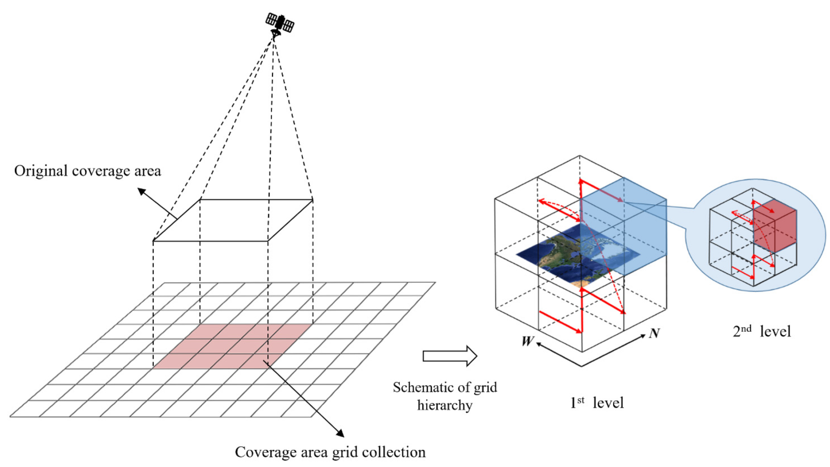
Different levels correspond to different sizes of spatial grids in the GeoSOT model. The essence of coverage area grid characterization is to discretize the area. We divide the coverage area into a series of grids through the GeoSOT model, and use the grid set to represent the coverage area. For different application scenarios, we select different levels of grids to divide the coverage area. The coverage area grid characterization is firstly a formal description, which introduces a dissecting grid to describe the representation form of the satellite ground coverage area and provides a basic logical reference for concrete implementation. Secondly, the characterization is a computational framework, which obtains the ground coverage area of satellite at a specific moment by the existing coverage calculation method, then dissects it to form a coverage grid, and then introduces a time dissecting code to expand the specific moment to any time period to form a satellite space-time coverage grid.

The grid characterization method is to select the highest grid level that meets the accuracy requirements of satellite applications, dissect the calculated satellite ground coverage area into this grid level and obtain a collection of grids (Figure 2). The satellite coverings of several different shapes at moment t are each dissected by the Nth level, assuming a number n, and the notation is in order $\left\{gri{d}_1,gir{d}_2\dots ,gri{d}_n\right\}$. Then, we use this collection to characterize the satellite ground coverage at this moment, i.e.,

$$C_{s,t\to e}\to \left\{gri{d}_1, gri{d}_2,\dots ,gri{d}_n\right\}$$

(1)

The notation in Equation (1) means mapping. In the GeoSOT profiling reference framework, all grids at all levels are uniquely coded. We named $gri{d}_n$’s code as $gcod{e}_n$, and for the satellite at moment t, its ground coverage $C_{s,t\to e}$ can be encoded as $G_{s,t\to e}$, i.e.,

$$\left\{\begin{array}{c}{C}_{s,t\to e}\to G_{s,t\to e}\\ G_{s,t\to e}=\left\{gcod{e}_i\right|C_{s,t,i}-gcod{e}_i, C_{s,t,i}\subset C_{s,t\to e}\}\end{array}\right.$$

(2)

In Equation (2), $C_{s,t,i}$ are the covered subregions that are consistent with the spatial extent of grid $gri{d}_i$ or conform to the boundary treatment principles.

The grid conversion Algorithm 1 for the coverage area is shown below:

Algorithm 1 Coverage area grid conversion algorithm

Input: Boundary Point Sequence $CoverLine\_pt\_seq$

Output:$\left\{gcod{e}_{border}\right\}$ and $\left\{gcod{e}_{inner}\right\}$

1: Traverse the boundary nodes of the spatial object $O$,

2: convert each node in turn to a node code with a profile level of n-level

3: record the inclusive box grid range $R$ of the boundary nodes

4: generate an $m\times n$ inclusive box grid matrix, when $j=n$, $Vij=-1$, else, $Vij=0$.

5: fill the node grid code $Cod{e}_i$ with $Cod{e}_{i+1}$ in turn, generate the boundary grid set $\left\{gcod{e}_{border}\right\}$.

6: set the value of the corresponding grid element in $V$ to 1 according to the boundary coverage processing rules, and set i = 1

7: while $i<R$

8:  Set flag $Flag=Flase$ and visit elements $V_{ij}$ in matrix $V$ one by one from left to right:

9:  if $V_{ij}=1$ and $V_{i,j+1}=0$, then

10:   Flag = true

11:   end if

12:   if $V_{ij}=0$ and $Flag=true$, then

13:     Let $V_{ij}\in \left\{gcod{e}_{inner}\right\}$

14:    end if

15:    i = i + 1

16: End while

17: return $\left\{gcod{e}_{border}\right\}$ and $\left\{gcod{e}_{inner}\right\}$.

The traditional satellite and ground base station coverage-area calculation methods cannot provide a unified description of different types of satellite observations, making it difficult to judge the spatial relationship between observation targets and coverage areas. The grid modeling of satellite range by GeoSOT can effectively solve the problem of uniform characterization of the coverage grid. Through layer selection, the grid size of each layer can just cover the application requirements of the satellite orbit and user terminal. While ensuring the accuracy of representation, it avoids the costs of data storage and computation of too-fine grids.

2.2. Calculation of Satellite-Ground Visibility

The satellite information transmission system generally consists of a space segment and a ground control segment, and information transmission can be carried out only after the establishment of a satellite-ground link. In the process of satellite motion, the satellite is in dynamic motion relative to the terminal, which poses difficulties for real-time calculation of the relative position of the satellite and the ground. In this section, we will establish a satellite grid computational model based on the GeoSOT model to solve the satellite selection problem in satellite-ground communication under the maximum service time.

The spatial reception area coverage of the ground terminal can also be expressed by using the ground coverage grid framework of the satellite.

Each satellite in the satellite constellation moves according to a certain orbit, and satellite trajectories can be calculated based on satellite orbit dynamics. Therefore, by mapping the satellite motion trajectory information with the sensor coverage area information in the GeoSOT grid coding system, we can perform grid modeling (Figure 3). The satellite motion trajectory is mainly composed of a series of ordered spatial 3D points. Under the grid coordinate system, we map the satellite’s latitude and longitude positions into a series of grid codes by determining the size of a specific grid. The motion speed of a low-orbiting satellite is about 7.5 km/s, so depending on the satellite response time, a GeoSOT grid with 9–15 levels is generally used for modeling.

Grid modeling for satellite beams, terminals, etc., is mainly used to calculate their coverage areas (Figure 2). By determining the boundary information of the coverage area, we can dissect the original coverage area and generate a collection of grids at the base level. This can then be aggregated according to the actual requirements to generate multi-scale grid codes and establish a one-to-many mapping relationship with temporal information.

In the model proposed in this paper, we use the distance of the satellite relative to the center of the terminal receiving area to determine whether the satellite is in the communicable range of the ground terminal. For a deterministic satellite, we know the orbital altitude, and the space coverage area of the ground terminal is a closed inverted conic surface body. As shown in Figure 4, the bottom of the inverted conic surface body can be projected onto the surface of the Earth, forming a closed surface region S. S is a circular area of radius r centered on the ground measurement and control station, and the circular area is the coverage area of the ground terminal for orbit height H.

Gridding the coverage area S, we have:

$$C_{u,H}\to \left\{gri{d}_1, gri{d}_2,\dots ,gri{d}_n\right\}$$

(3)

Further onwards,

$$\left\{\begin{array}{c}{C}_{u,H}\to G_{u,H}\\ G_{u,H}=\left\{gcod{e}_i\right|C_{u,H,i}-gcod{e}_i, C_{u,H,i}\subset C_{u,H}\}\end{array}\right.$$

(4)

Equation (4) is the form of the grid code description of the coverage area of the ground terminal for orbit height H.

The primary condition for establishing a stable satellite-ground link is to be within the visibility range of the terminal, followed by the state of motion of the satellite equivalent to the center of the terminal. Because the visibility of the ground terminal and the satellite is mainly related to the angle of the satellite relative to the terminal, the distance will hardly affect the visibility of the satellite signal, but will affect the strength of the signal. Additionally, within the same altitude layer, the distance L between the satellite and the center point is the key factor for measuring whether the satellite is within the acceptance range. Therefore, converting the position analysis of the satellite and the location station to the position analysis of the ground terminal centroid projection and the satellite can convert the three-dimensional position calculation into a two-dimensional plane. Compared with judging the spatial relationship between the satellite and the terminal by calculating the angle of the satellite relative to the terminal, this paper makes a judgment of the relative position and motion state of both by the change in distance L, i.e.,

$$L=Gri{d}_{satelite}-Gri{d}_{central}$$

(5)

$$L<H\times \frac{tan\theta }{L_{Grid}}$$

(6)

$$∆L<L_t-L_{t+1}$$

(7)

$\theta$ is the maximum elevation angle fixed by the terminal, $H$ is the altitude of the current satellite and $t$ is the current satellite time. (1) $L$ is the distance between the grid-calculated satellite and the center point; (2) it indicates a rough judgment method within the acceptance range of the terminal, as long as L is less than the coverage boundary; and (3) it can indicate the motion state of the satellite relative to the center point.

In the GeoSOT model, the grids at the same level have the same volume size, so the distance between two grids can be represented by the number of grids. We represent the distance between satellites by the difference in the distance between grids, thus we can judge the movement of the satellite’s position in the receiving area. As shown in Figure 5, after the satellite space is gridded, the number of grid differences between the satellite grid and the grid where the center point is located is calculated using the grid where the satellite is located, representing the position of the satellite. Because the satellite is in dynamic motion, as shown in Figure 6, the grid in which the satellite is in motion will also change, and the number of grids away from the centroid will also change.

In the GeoSOT grid calculation model we can obtain the following rules:

• The closer the position grid is to the edge of the receiving range, the greater the grid distance.
• The grid difference in two time intervals $∆t$ can indicate the motion state. The number of grids at moment t from the center point is greater than the number of grids at moment $t+1$, i.e., $N_t>N_t+1$, which roughly means that the satellite is moving to a position close to the center point.

Suppose the initial selection time is $t$, and the grid distance of satellite $A$ at this time is $N_{A-t}$. By analyzing the grid number from the center point during the motion of different satellites, we can set the following judgment model:

• If $N_t>N_t+1$, the larger $N_t$ is, the longer it stays in the receiving area, and the higher priority we set.
• If $N_t<N_t+1$, the smaller $N_t$ is, the longer it stays in the acceptance area, and the higher priority we set;
• The $N_t>N_t+1$ case is overall higher than the $N_t<N_t+1$ motion case.

The GeoSOT grid code is an integer binary three-dimensional code, and its bit operation between codes is faster, which can meet the demand of fast response between multiple objects. With the position calculation model proposed in this section, we can use the grid bit operation to directly express the position relationship between the satellite and the terminal, and achieve the goal of fast calculation of the satellite-ground position relationship.

3. Experiment and Result

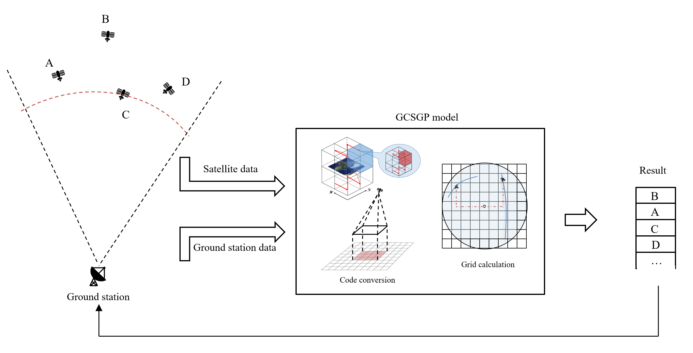
In order to validate the proposed GCSGP model in this paper, we develop a feasibility verification experiment for selecting the longest service time satellite using grid computing. In addition, we also validate the computational accuracy error and time efficiency of the GCSGP model. The overall experimental architecture is shown in Figure 7.

3.1. Feasibility Experiments

In the feasibility experiment, we use the real BeiDou satellite orbital root and terminal data as the basic experimental data. In order to show the experimental results more intuitively, we choose the following satellites in the three orbital planes of the Big Dipper constellation for the experiment, with a simulation start time of 20:00:00 on 23 May 2021 and end time of 02:00:00 on 24 May 2021. The simulation duration is 6 h, and the time interval is 10 s for each simulation (

Table 1. Satellite data for experiments.

Satellite	Terminal	Test Time
BEIDOU 10 (C10) BEIDOU 17 (C31) BEIDOU 7 (C07) BEIDOU 20 (C18)	Properties of the simulated terminal: (Lat: 39.9989 deg Lon:116.317 deg Height: 0 m) Cone Half Angle: 45 deg	20210523-20:00(UTM+8)–20210524-2:00(UTM+8)
BEIDOU-3M9(C23) BEIDOU-3 M11 (C25) BEIDOU-3 M10 (C24) BEIDOU-3 M12 (C26)
BEIDOU 9 (C09) BEIDOU-3IGSO-2 (C39) BEIDOU IGSO-7 (C16) BEIDOU 5 (C06)

).

In our experiments, we use the satellite orbit data to generate satellite motion grid data based on the satellite within the test window, and use STK to simulate and verify the BeiDou satellite constellation model to simulate the generation of the link between the satellite and the terminal.

The experimental steps are as follows.

Step1: Use the GeoSOT grid model to grid the satellite trajectory data to produce grid coordinates;

Step2: Use the model in Section 2.2 to calculate the grid positions of satellites and terminals and rank the satellites according to the results;

Step3: Use the STK software satellite and terminal link for simulation;

Step4: Compare the results of grid calculation with the results of simulation.

3.2. Analysis of Grid Computing Feasibility Results

According to the GeoSOT encoding model, we apply grid encoding to the position of satellites and the terminal. After that, by calculating the grid encoding, we can obtain the grid distance between the satellite position and the terminal position at each time step, as shown in Figure 8.

Two features should be noticed in Figure 8. One is the grid distance of each satellite, shown on the y-axis. The larger the grid distance, the closer it is to the edge of the coverage area. The other feature is the variation in grid distance, which we can obtain from the slope of each satellite’s grid distance curve. If the curve has an upward trend, which means the slope of the curve is greater than zero, it indicates that the satellite is moving away from the coverage area. Therefore, a curve with a large initial grid distance and slope less than zero will represent a satellite with long residence time. A curve with a large initial grid distance and slope greater than zero will be a satellite that leaves the coverage area fastest.

From the result graph in Figure 8, we can see that:

• IGSO_43603 (blue line) has the highest initial grid distance, but the grid distance of the satellite is still increasing as time increases, indicating that IGSO_43603 is at the edge of the detection region, while still accelerating away from the detection region, so we drop its ranking to the last.
• Among the remaining candidate satellites, IGSO_37256 (purple line) has the highest initial grid distance, while the grid distance of the satellite is decreasing with time, and it has not yet reached the nearest position turning point.
• IGSO_36828 (green line) reaches the distance nadir at the second time node, after which it starts to run away from the detection center.

With the experimental results, we can rank the satellites according to the available time as follows: IGSO_37256 > IGSO_37763 > IGSO_43581 > IGSO_44337 > IGSO_43539 > IGSO_36828 > IGSO_43603.

Using the same satellite and terminal data in STK software, we can generate the experimental results as shown in Figure 9.

The y-axis represents different satellites, and we use different colors to distinguish them. The x-axis represents the time interval. Each horizontal line represents the coverage time interval of each satellite. Take satellite IGSO_44337 as an example, which is located at the bottom of Figure 9 and is represented in red. This indicates that the link time of the satellite in the coverage area is from 20:00 to 00:20 on the 24th. The simulation results can visualize the link time between the observation satellite and the ground terminal. By ranking the longest link time, we can make a comparison with the grid calculation ranking results. The simulation results of the satellite-ground link in Figure 9 can show more intuitively that satellite IGSO_37256 has the longest visibility time throughout the whole calculation period, followed by satellite IGSO_37763, and the satellite IGSO_43603 has the smallest visibility time. The results for the longest satellite link time are approximately the same as those obtained from our grid calculations.

3.3. Accuracy and Computational Efficiency Analysis Experiments

In terms of the accuracy and computational efficiency of the GCSGP model, we will analyze the effect of satellite altitude and receiver elevation angle on the accuracy of the experiment under a grid of 9–15 size level. Under the fixed variables of altitude and elevation angle, the accuracies of the grid coordinates with respect to latitude and longitude at a certain level are tested by selecting the coordinates of a fixed distance from the center point and the coordinates of the point at the edge of the receiver range, respectively.

The use of the grid instead of latitude and longitude will certainly bring up some errors in spatial position representation. The GeoSOT grid will produce different errors at different layer scales. In this experiment, we take satellite BEIDOU-3M9(C23) as an example, and analyze the accuracy error at different levels under two factors of satellite altitude and receiver angle.

From Figure 10, we can see that the error of the grid at level 9 is larger when the altitude is below 2500 km, and the error decreases significantly when the altitude is higher; grids of 10–15 levels are available with the required accuracy at the test height of the satellite distribution.

From Figure 11, it can be learned that the larger the angle at the same height, the larger the critical edge distance of the center point of phase convergence at a fixed height, and the smaller the area share of the unit grid area at that height, and the system error will be reduced. At the same time, for receivers with small inclination angles, the use of grids tends to cause larger computational errors. Using a higher-level grid (e.g., 14 levels) can result in better performance.

We compare the calculation time of satellite-ground position using latitude and longitude coordinates with that using grid coordinates. We generate 10,000 to 10,000,000 satellite trajectory points, calculate GeoSOT-3D codes for each point at 9–15 levels and perform the following operations separately.

A. Calculate the Euclidean distance between N trajectory points and the terminal and record the calculation time.

B. For N trajectory points (same as in A), use their grid coordinates to calculate the grid distance between the satellite position and the terminal, and record the time.

Figure 12 shows the total time consumed by conventional GPS for spatial distance calculation and grid distance calculation. We choose the grid of the 10th level for satellite position characterization. It can be seen that the grid code calculation time is lower than that of the conventional latitude and longitude.

The experimental results in Figure 12 show that the total time consumed for grid distance calculation is much smaller than that of the traditional latitude and longitude approach, and the time calculation is reduced by about 7 times, mainly because the use of grid code calculation avoids the conversion of polar coordinates and a large number of trigonometric and square calculations, which reduces its complexity.

4. Discussion

Compared with traditional characterization, grid characterization has the following advantages.

(1) The traditional model is inconsistent in the basic unit of satellite ground coverage capability representation, and it is unable to unify the expression of different types of satellite observation resources, while the GeoSOT coding-based grid dissection model takes the geospatial grid as the basis, quantifies the ground coverage capability of observation resources into a spatial grid, appends the temporal information to form a temporal-spatial grid of satellite resources and finally uses a unified coding model to characterize the spatio-temporal grid, which can realize the unified expression of multiple types and large numbers of space and Earth resources.

(2) The traditional model cannot intuitively determine whether the observed target is within the satellite’s ground coverage range. Since the current discrete subsatellite trajectory and load width are simply used to characterize the satellite’s observation capability, when judging the spatial relationship between the observed target and the satellite’s ground coverage range, it is necessary to abstract the line and surface-shaped observed target into a point, and calculate and judge whether the distance from the point to the subsatellite trajectory is within the load width. The distance from the point to the subsatellite trajectory is calculated and determined to be within the payload width. The literature reference in [20] is about position calculations based on the specific position of the satellite in relation to the receiver, followed by pseudo-range observations. When the observation task is heavy, the computation time should not be underestimated. In contrast, the GCSGP model uses a spatio-temporal grid (collection) to visually represent the ground coverage, and the spatial relationships are more efficient. With one million positions, the traditional calculation takes 0.72 s, while the grid calculation takes only 0.12 s.

However, the use of grid coordinates instead of latitude and longitude coordinates improves efficiency, but gives up some accuracy. In the altitude accuracy experiment in Figure 10, we set the receiver inclination angle to 45° and tested the grid error test from a 500 km to 20,000 km altitude. The results show that the grid of 10–15 levels can achieve an error within 1% at all altitudes, and shows a decreasing trend with increasing altitude. In the angular accuracy experiments in Figure 11, the error decreases with increasing receiver inclination; for example, in the ninth-level grid, the error is 7.3% at 10° inclination, while the error is only 1.3% at 45° inclination.

In both the height and angle accuracy test results, we found that the error of the test decreases as the grid level increases. This is because the larger the number of dissection levels, the smaller the grid cell size, so the more accurately the coverage grid at the boundary can fit the original coverage boundary. The characterization accuracy is thus improved. As is shown in Figure 13, the blue area is at the boundary of the ground coverage area, and the red object is the dissection grid, with the number of dissection levels increasing from left to right. For level $A$, the grid drawn on the left is a covering grid according to the principle of covering boundary determination. For level $A+1$, the four subgrids of this grid are also covering grids, but for the profiling level $A+2$, seven of all the subgrids of the four subgrids of this grid are not covering grids.

This paper proposes a grid calculation model for satellites on the ground, mainly to provide solutions for rapid interconnection and information interaction of satellite constellations for large-scale and complex network communications in low orbit. Because the GeoSOT grid has two-dimensional and three-dimensional consistency, it can provide effective support for ground, satellite-ground and inter-satellite computations, and is conducive to the construction of a unified and integrated computing network between space and Earth. This paper is also the first to apply the grid system to the calculation of satellite-ground position, and there are still many problems in the application that deserve in-depth study. For example, the influence of weather and atmosphere on signal transmission, the satellite selection strategy and signal transmission routing, the scheduling of on-board resources and the optimization of on-board algorithm storage will be further studied in the future.

5. Conclusions

Combined with constellation groups such as BeiDou satellites, this paper introduces the GeoSOT model and applies it within the aerospace field to explore a spatially fast calculation method of satellite links. By using the GeoSOT model to discretize the Earth’s space, the GeoSOT-based grid calculation model for satellite-ground position model is constructed, and the angular calculation of longitude and latitude floating point numbers is replaced by the number calculation between grids. A grid data judgment model in terms of the longest service time of satellites is formed. We start with the grid coding of satellite trajectories, then calculate the grid distance between satellites and ground using grid coding algebra, rank and classify the optional satellites and then verify the feasibility and accuracy of the experimental results via STK simulation. On the basis of verifying the correctness of the model, the accuracy of the grid calculation method was verified and the time efficiency of the traditional latitude and longitude calculation method was compared with that of the grid calculation method. It is about 82% faster than the traditional latitude and longitude calculation method on the basis of a single constellation calculation. In future research, we plan to add improvements and undertake further experiments. Firstly, the current environment of our test is relatively simple; the real situation will be more complex, so more variables and constraints will be added in future research. Secondly, we will also conduct more levels of comparison with other studies to further explore the advantages and disadvantages of grid computing. Finally, there are thousands of satellites in the low-orbit constellation, and the subsequent research will analyze the scheduling applications of this full constellation of satellites in specific application scenarios.