Article

UAV Remote Sensing for Detecting within-Field Spatial Variation of Winter Wheat Growth and Links to Soil Properties and Historical Management Practices. A Case Study on Belgian Loamy Soil

1
Territory and Technologies Unit, Walloon Agricultural Research Centre (CRA-W), 5030 Gembloux, Belgium
2
Georges Lemaître Centre for Earth and Climate Research, Earth and Life Institute, Université Catholique de Louvain (UCL), 1348 Louvain-la-Neuve, Belgium
3
Crop Production Unit, Walloon Agricultural Research Centre (CRA-W), 5030 Gembloux, Belgium
4
General Direction, Walloon Agricultural Research Centre (CRA-W), 5030 Gembloux, Belgium
*
Author to whom correspondence should be addressed.
Remote Sens. 2022, 14(12), 2806; https://doi.org/10.3390/rs14122806
Submission received: 14 April 2022 / Revised: 23 May 2022 / Accepted: 8 June 2022 / Published: 11 June 2022
(This article belongs to the Special Issue Innovative Belgian Earth Observation Research for the Environment)

Abstract

:
Intra-field heterogeneity of soil properties, such as soil organic carbon (SOC), nitrogen (N), phosphorous (P), exchangeable cations, pH, or soil texture, is a function of complex interactions between biological factors, physical factors, and historic agricultural management. Mapping the crop growth and final yield heterogeneity and quantifying their link with soil properties can contribute to an optimization of amendment/fertilizer application and crop yield in a management variable zones (MVZ) approach. To this end, we studied a field of 17 ha consisting of four former fields that were merged in early 2017 and cropped with winter wheat in 2018. Historical management practices data were collected. The topsoil characteristics were analyzed by grid-based sampling and kriged to create maps. We tested the capacity of a multispectral MicaSense® RedEdge-MTM camera sensor embedded on an unmanned aerial vehicle (UAV) to map in-season growth of winter wheat. Relating several vegetation indices (VIs) to the plant area index (PAI) measured in the field highlighted the red-edge NDVI (RENDVI) as the most suitable to follow the crop growth throughout the growing season. The georeferenced final grain yield of the winter wheat was measured by a combine harvester. The spatial patterns in RENDVI at three phenological stages were mapped and analyzed together with the yield map. For each of these images a conditional inference forest (CI-forest) algorithm was used to identify the soil properties significantly influencing these spatial patterns. Historical management practices of the four former fields have induced significant heterogeneity in soil properties and crop growth. The spatial patterns of RENDVI are rather constant over time and their Spearman rank correlation with yield is similar along the growing season (r ≃ 0.7). Soil properties explain between 87% (mid-March) to 78% (mid-May) of the variance in RENDVI throughout the growing season, as well as 66% of the variance in yield. The pH and exchangeable K are the most significant factors explaining from 15 to 26% of the variance in crop growth. The methodology proposed in this paper to quantify the importance of soil parameters based on the CI-forest algorithm can contribute to a better management of amendment/fertilizer inputs by stressing the most important parameters to take into consideration for site-specific management. We also showed that heterogeneity induced by the soil properties can be described by a crop map early in the season and that this crop map can be used to optimize soil sampling and thus amendment/fertilizer management.

1. Introduction

According to the Food and Agriculture Organization (FAO), the demand for cereals will increase by 70% by 2050 due to an ever-growing population [1]. Currently, croplands under conventional management receive broadcasted applications of fertilizers, herbicides, irrigation, seeds, etc. [2], while it has been shown that soil properties and crop conditions can vary considerably over space and time within a single field [3]. In order to secure food supplies for future generations, expected amounts and quality of agricultural products, intensive but environmentally safe production, and sustainability of the resources involved are required. To meet these ends, precision agriculture emerged as a way to apply the right treatment type and amount in the right place at the right time [4]. Gebbers and Adamchuk [4] defined precision agriculture as “ [agriculture that] comprises a set of technologies that combine sensors, information systems, enhanced machinery, and informed management to optimize production by accounting for [spatial and temporal] variability and uncertainties within agricultural systems”. Hence, when precision agriculture is applied to a field, it is potentially divided into various management zones that each receive customized inputs, based on landscape position and soil conditions [2].
Spatial distribution of crop growth and yield within a territory are classically expected to result, besides crop management, from basic factors such as soil characteristics, position in the landscape (field topography and soil exposure), and weather conditions. Understanding the degree of importance of the effects of these main drivers on crop growth and yield is essential in order to assess the potentialities and usefulness of applying variable rate inputs, mainly amendments (organic or calcic) and fertilizers, within a field [5]. The most relevant properties of soil productivity are soil moisture content, clay content, organic matter content, nutrient availability, pH, and bulk density [4]. However, spatial variations in crop yield reflect not only the influence of soil properties, site characteristics, and weather conditions, but also their complex interactions. Therefore, seasonal variation in crop growth conditions such as water stress or excess, lack or excess in nutrients, and disease, pest, and weed pressures and incidences can also greatly affect inter- and intra-annual variations in crop performance [6]. The intra-field heterogeneity of soil properties is thereby a function of complex interactions between biological, physical, and chemical factors as well as historical management practices.
Remote sensing in agriculture allows non-contact measurements of spectral radiation reflected from crop canopy or bare soil, and has been used since the early 1970s (for an exhaustive list of studies see [2]). With the development of remote sensing technology leading to increasing spatial, temporal, and spectral resolution, the relevance of using reflectance data from remote platforms has increased [2]. These technological advances in remote sensing imagery coupled with a decrease in associated costs have allowed the collection of timely information on crop variability. Such information on agricultural crop status during the growing season can be used for estimating potential crop yields. Moreover, an early assessment of the risk of yield reduction acquired by timely crop monitoring could help to guide the strategic planning related to site-specific management of crop inputs, such as amendments or fertilizers. Remote sensing is frequently used to estimate spatial patterns in crop growth through the use of spectral vegetation indices (VIs), such as the commonly used Normalized Difference Vegetation Index (NDVI). However, the latter suffers from limitations when it comes to estimating the total plant biomass in fully developed crops, and the use of other spectral indexes, such as those including the red-edge bands (centered around 740 nm), is recommended [7].
Recently, unmanned aerial vehicles (UAV) have been developed as low-cost observational platforms for environmental monitoring with an ever-increasing scientific interest [8]. The latest advancements in sensor specifications (weight, spectral and radiometric resolutions, battery autonomy) have allowed an exponential increase of UAV applications in agriculture, as they can be easily deployed to monitor the crop during the growing season over a field or some contiguous fields.
Numerous studies have described crop growth monitoring through the use of such technologies combining remote sensing and UAVs. Lukas et al. [9] showed that Green NDVI (GNDVI) is a reliable variable to estimate winter wheat biomass across the growing season. Schirrmann et al. [10] showed that RGB UAV imagery is sufficient to assess winter wheat crop biophysical variables such as leaf area index (LAI) along the growing season and that there is significant variation in pattern between different dates. Barley biomass estimation can be made by combining RGB height estimation and VI. While only VI is suitable at early development stages, the combination with RGB height is more robust at advanced stages [11].
This paper aims to explore the links between the within-field spatial variations in crop growth throughout the growing season and the spatial variability of site characteristics, current soil properties (physical and chemical), and contrasted historical soil and crop management practices. We use a case study of a winter wheat crop in 2018 (sowing in autumn 2017) in a single loamy field of central Belgium (Gembloux). Crop growth assessment was based on relevant VIs derived from in-season UAV remote sensing imagery and yield mapping sensor at harvest. Information on the current within-field spatial patterns of soil characteristics, such as soil organic carbon (SOC), nitrogen (N), phosphorus (P), exchangeable cations, pH, or physical soil texture characteristics, were collected. The objectives of the present study were (i) to test a selection of UAV-based VIs and choose the best one to accurately monitor and map in-season winter wheat crop growth heterogeneity as well as the related final grain yield; (ii) to assess, using a conditional inference forest (CI-forest) algorithm, the link between, on the one hand, the winter wheat crop growth and yield, and on the other hand, field soil properties, characteristics, and former field layout linked to contrasted historical soil and crop management practices within four previous different parcels merged into a unique field; (iii) to explore and discuss the possibilities of UAV remote sensing acquisition on a winter wheat canopy growth and yield to indirectly qualify and/or quantify the within-field spatial patterns of soil properties and characteristics, and to define potential field management variable zones. Such final information could contribute, for instance, either to an improvement in the optimization of further amendments, manures or fertilizer recommendation aiming to mitigate soil heterogeneity effect on crop, or to better contribute to in-season management of fertilizer application through site-specific management of the crop.

2. Materials and Methods

2.1. Study Site

The study was conducted in 2018 on an experimental conventional farming field (50°33′55.0″N, 4°43′02.2″E) in the vicinity of Gembloux, central Belgium. The field is located in the loam belt region dominated by niveo-eolian deposits characterized by well-drained soils. The climate is temperate oceanic with mean annual precipitation of 790 mm and with the lowest monthly mean temperature in January (2.3 °C) and the highest monthly mean temperature in July (17.8 °C). The field of 17 ha consists of four former parcels, characterized by contrasted historical soil and crop management practices, that were merged in spring 2017. The entire field was sown with a winter wheat crop in October 2017 (Figure 1). The study area was defined within this field by applying an inner buffer of five meters to avoid the border effects in the analysis of the UAV images, manually deleting the headlands, and keeping only the area covered by the three UAV images captured during the 2018 winter wheat crop growing season (cf. Section 2.3).
A calendar of annual field management practices for the four parcels of the former field layout dating back to 1990 was established. The data collected concerned main crop, organic and mineral amendments and fertilizers, cover crops, and residues, all of which affect the soil organic and mineral content. P, K, Mg, and Ca fertilizer/amendment contents (obtained from laboratory analysis or internal references for organic or calcic fertilizer/amendment) were used to calculate/estimate the rates applied. An estimation of the exportation of P, K, and Mg at harvest was carried out using yield, crop type, and P–K–Mg exportation (kg per yield unit) [12]. Daily meteorological data from the Belgian Royal Meteorological Institute (RMI) weather station (Gembloux-Ernage) located within 3 km from the field were retrieved from March to July 2018. Temperature and precipitation data were used to assess the growing conditions.

2.2. Soil Data

A total of 80 soil samples (0–25 cm depth) were collected in August 2018 according to a systematic sampling design on the nodes of a 50 m grid. Each sample consisted of 10 subsamples taken within a radius of 2.5 m with a 3 cm diameter core drill. Sample positions were recorded using a John Deere Starfire 3000 Real Time Kinematic (RTK) GPS instrument (Moline, IL, USA) with 2.5 cm precision. The samples were dried (<40 °C) and gently crushed and passed through a 2 mm sieve, according to NF ISO 11464 standard, and analyzed for soil organic carbon (SOC), total nitrogen (N), P, Fe, Ca, exchangeable cations (K, Mg, Mn), pH, and soil texture (Table 1). To assess the importance of the former field layout on the variability of soil properties, a one-factor analysis of variance (ANOVA) test was applied for each soil variable, using the former field layout as the categorical factor of interest. This test was followed by a Student–Newman–Keuls (SNK) test (alpha value of 0.05) to identify, for each variable, the significantly different former field(s).
Additionally to the soil properties analysis, a digital elevation model (DEM) at 1 m spatial resolution was downloaded from the Walloon Geoportal, an online geodatabase of the Walloon region. The DEM was generated from aerial light detection and ranging (LiDAR) images acquired between December 2012 and March 2014. The average point density of the scanner is less than 1 point/m2, and the altimetric resolution is ca. 0.12 m over the entire Walloon territory (source: http://geoportail.wallonie.be/catalogue/6029e738-f828-438b-b10a-85e67f77af92.html; accessed on 10 March 2022).

2.3. Crop Data

Crop growth was assessed based on the plant area index (PAI) derived from ground-truth digital hemispherical photography (DHP) and VIs derived from UAV multispectral imagery. UAV images and DHP were acquired at three dates during winter wheat growing season: 26 March 2018 (BBCH phenological stage 28, end of tillering), 17 April 2018 (BBCH 30, beginning of stem elongation), and 16 May 2018 (BBCH 37, end of stem elongation).
DHP technique uses a digital camera with a fisheye lens to measure canopy gap fraction over a wide range of viewing directions [14]. This technique is widely used and allows retrieving LAI with an uncertainty of less than 1 [15]. A BESEL Super fish-eye lens 0.25× was mounted on a CANON Powershot A540 (Tokyo, Japan) camera set on a 1200 × 1600 pixel per image resolution. Photographs were taken in a downward-pointing direction at about 1.5 m distance from the ground on a regular basis by following the tractor tracks (north–west–west orientation). Each point corresponds to the central position of a series of ten pictures spaced one step apart (Figure 1) and was geolocated with a Spectra Promark 120 L1 RTK GPS. CAN-EYE software [16] was used to process the DHP pictures and to derive one PAI value per series. PAI is very similar to LAI for winter wheat.
A RedEdge-MTM sensor from MicaSense® (Washington, DC, USA) was used to acquire UAV multispectral images of the crop. It allows capturing images in five narrow spectral bands, each from a dedicated sensor, in the range 475–840 nm (Table 2). Images are provided with a resolution of 1280 × 960 pixels, from a sensor with a horizontal field of view (HFOV) of 47.2 degrees. The image acquisition rate was fixed at 1 image/second. Sensor sensitivity and exposure time were set to automatic for each picture. The camera was integrated with a downwelling light sensor, provided by MicaSense®, to register solar irradiance for each picture and allow for radiance correction in post-processing.
For data acquisition, the RedEdge-MTM was embedded on a quadcopter-type UAV (a DJI Phantom 3 and a custom-made model with DJI N3 controller). UAV surveys were executed with flight planning software (DJI Ground Station Pro; Shenzhen, China) to keep a regular flight elevation of 45 m a.g.l., a regular inter-line distance to provide a lateral overlap of the images of 80%, and a flight speed of 6 m s−1 to provide a frontal overlap of 80%. Pictures of a calibrated reflectance target were acquired at the beginning of each flight to allow for conversion of radiance data to reflectance.
The images were then processed with the photogrammetric software Pix4d Mapper (Lausanne, Switzerland) to produce reflectance maps with a resolution of 3.9 cm/pixel. This software automatically dealt with all of the phases of image correction (black-level compensation, vignetting correction, radiometric calibration), orthomosaic generation, and data conversion from radiance to reflectance.
In addition, the grain yield was measured during the harvest on 17 July 2018 using a force plate sensor (impulsion measurement) embedded on the combine harvester. The yield sensor from John Deere was placed in front of the hopper and measured the grain flow (number of grains per second). The grain flow value was then converted into yield. The average harvesting width was 7.1 m and the system recorded data every 1.3 m. Geolocation was recorded with a John Deere Starfire 3000 RTK GPS. The data were supplied already interpolated at 1 m resolution by ordinary kriging (OK).

2.4. Data Analysis

2.4.1. Vegetation Indices

Aiming at characterizing the heterogeneity of the crop growth at the three UAV images acquisition dates, four VIs were computed using the spectral data provided by the RedEdge-MTM sensor (Table 2). All VIs were calculated in the form of a generic normalized difference index (NDI) combining the near-infrared (NIR) band with the red (R), green (G), and red-edge (RE) bands, except for the NDI668-717, which combines the R and RE bands (Table 3). The VI with the highest capacity to characterize crop growth heterogeneity was selected, taking into account (i) the capacity to avoid saturation, to which some VIs are sensitive [17], and (ii) the goodness of fit of its relationship to PAI, which is used as ground-truth data. A simple linear regression was carried out on PAI and the VI values extracted within a 1 m buffer area of the corresponding locations. An additional manually created mask was applied to erase the tractor tracks.

2.4.2. Compilation of Uniform Maps

In order to provide uniform information into the final model and to reduce computation time of the operation, all the geolocated data available were transformed to fit a reference grid of 10 m resolution. This resolution was considered as adequate to correlate crop patterns with soil properties determined from samples spaced 50 m apart. Additionally, even with this resampling resolution, UAV-based crop images are still useful because the reflectance of aggregated pixels is more accurate than 10 m resolution satellite images, where a single pixel still has, to some extent, the influence of the reflectance of the neighboring pixels, while the aggregation of fine-resolution pixels minimizes uncertainty due to georeferencing.
The VI, yield, and DEM rasters were aggregated and resampled by means of the bilinear interpolation technique to fit the 10 m resolution reference grid. This method assigns the output cell value by taking the weighted average of four closest cell centers. The previous parcel layout (the only categorical variable) was rasterized to the reference grid.
The soil physicochemical properties were interpolated according to the reference grid using OK. Within the variety of interpolation methods for soil parameters, OK was proven to be performant for application in crop-site-specific management [21,22]. It takes into consideration both the distance and the degree of variation among known points when calculating the unknown points and it estimates a value at a point of a region for which a variogram has been fitted [23]. Grid sampling method is preferred to random sampling for this kind of purpose [24], and a good knowledge of spatial dependence of the soil variables considered is important as a strong dependence makes it easier for site-specific management [25]. The basic parameters required for OK prediction are supplied by a variogram 2γ(x,y). It is a function describing the spatial dependence of a random field, and it is defined as the expected square increment of the values between locations x and y [23]. The variograms were fitted using the fit.variogram function in R v3.6.1 (R Core Team, Vienna, Austria) gstat v1.1-6 package, for all soil variables. The fitted spherical variogram models were subsequently used in the OK krige function in R gstat v1.1-6 package, and the selected soil variables were interpolated according to the 10 m resolution reference grid. The sill-to-nugget ratio was calculated to evaluate the quality of the semivariograms, and a leave-one-out cross-validation procedure was conducted to compute a relative root mean square error of cross validation (rRMSECV; i.e., RMSECV divided by the mean) to assess the quality of the interpolation.
Overall, the final dataset contains rasters of VI at three dates (26 March 2018, 17 April 2018, and 16 May 2018), yields, DEM, former field layout, and soil physicochemical properties at 10 m resolution.

2.4.3. Conditional Inference Forest

A CI-forest algorithm was used to identify, amongst the DEM, former field layout, and soil properties variables, the key drivers of crop growth at the four development stages (in March, April, and May for crop vegetation growth and in July at harvest for yield). The CI forest algorithm is a tree ensemble machine learning procedure similar to a random forest (RF). It combines the growth of multiple CI-trees to produce a more stable and accurate regression compared to a single CI-tree, by eliminating the possibility of overfitting the original data (i.e., the fitted model corresponds too closely to a particular dataset and might therefore fail to fit additional data) [26]. Moreover, it is capable of modeling nonlinear interactions between response and predictor variables without any pre-assumptions about the distribution of the data [27,28]. The advantage of using CI-forest, compared to the traditional RF, is the decision to split a node, which is based upon the outcome of a test of the global null hypothesis of independence between the response and the predictor variables selected for splitting a node. If the null hypothesis is rejected at specified significance level, the node is split, otherwise, the tree growth is completed [29].
A total of 500 CI-trees were grown using the CI-forest algorithm (cforest() in the R v3.6.1 (R Core Team, Vienna, Austria) “party” package v1.3-3). The predictor variables used to construct the models included soil properties, information on the former field layout, and the digital elevation model (DEM). Empirical results suggest that the importance of correlated predictor variables is severely overestimated [30]. Therefore, when highly correlated predictors occur (Pearson’s rank correlation coefficient ρ > 0.7), the variable with lower rRMSECV, i.e., higher quality of interpolation, was selected so as to include a more accurate kriged map in the CI-forest model.
The number of splitting variables was set to half the square root of the total number of predictor variables. The criterion for partitioning was set at 0.95, i.e., the null hypothesis to split a node is to be rejected at the significance level α = 0.05. For each CI-forest model, the relative variable importance (RVI) was extracted. Variables were deemed important if their relative importance was greater than that expected from a theoretical model, where all predictors are equally influential [29]. The performance of the model was evaluated using the coefficient of determination (R2) and the RMSE.

3. Results

3.1. Historical Soil and Crop Management and 2018 Meteorological Conditions

Soil and crop management practices data for the period 1990–2018 across the parcels of the former field layout were retrieved from CRA-W archives and compiled to create a summary of the field management practices (Table 4 and Table 5). The four parcels were managed in a conventional farming system throughout the period 1990–2018. The values of Table 4 and Table 5 are presented for four sub-periods from 1990 to 2018 to allow the illustration of the contrasted historical soil and crop management practices and also the consideration of short- to long-term effects of such practices on current soil properties. For each sub-period, values are expressed as the sum of annual values over the sub-period. The crops were grown in rotation. The main crops are the main ones for central Belgium, i.e., winter wheat (Triticum aestivum sp.), winter barley (Hordeum vulgare sp.), sugar beet (Beta vulgaris subsp. vulgaris Altissima Group sp.), maize (Zea mays sp.), potato (Solanum tuberosum sp.), and oilseed rape (Brassica napus sp.).
The soil was ploughed and harrowed every year and usual crop protection products (fungicides, herbicides, insecticides) were used. Recommended N–P–K fertilization was applied according to the balance sheet method for N and the triennial balance between import and crop uptakes for P and K, applying various mineral or organic forms of fertilizers and amendments (organic or calcic).
SOC can be affected by the crop residue restitution, organic amendments (farmyard manure, slurry, waste lime), and winter cover crops (Table 4) [31]. Before 2009, mustard was occasionally sown as a winter cover crop. The last ten years, winter cover crops (ray-grass or mixture) were sown systematically if possible prior to a summer crop. Since 1990, there have been no remarkable differences between parcels for cover crops. Long-term observation of crop residues shows a higher occurrence on parcel D. Looking at least at the last ten years or more, more organic inputs were applied on plots B and D, which is expected to have increased their SOC content over the period.
Organic amendments also contain various amounts of minerals such as P, K, Mg, and Ca, also supplied by mineral fertilizers and amendments such as KCl, solid P–K in various proportions, Haspargit (K2O, CaO, SO3), or dolomite (CaCO3 and MgCO3).
For the 2014–2018 period, the balance between import and export of P, K, and Mg was negative, especially on parcel A (Table 5). For 2010–2018, the balance is positive for parcel B, close to zero for parcel D, and still negative for parcel A and C. This differentiation between the A–C and B–D parcels remains for the 2000–2018 period, especially for P and K.
Ca was supplied by organic amendment (especially waste lime), Haspargit, and dolomite, which are used to lime the parcel. Waste lime was applied until 2009. Haspargit was occasionally applied in the last 20 years on each parcel and the most recent application dates back to 2014 on parcels A and B. A total of 1500 kg·ha−1 of dolomite (55% CaCO3, 40% MgCO3) was applied on plot B in 2009. According to the 2010–2018 period, a higher pH can be expected on parcels B and D.
The four parcels were merged in spring 2017 into a unique field of 17 ha. Maize was then sown over the whole field with a N–P–K supply (21%–6%–6%) of 500 kg·ha−1 as bulk fertilizer and harvested in October. Winter wheat was sown on 27 October 2017 for the 2018 growing season. Only mineral N was supplied, with an application of 71.5 uN·ha−1 (sulfazote) in March and 60 uN·ha−1 (solid) in May (Figure 2).
According to the “Bulletins Agrométéorologiques” for the year 2018 [32], growing conditions were favorable for winter wheat at the end of winter and beginning of spring. May, June, and July were unusually dry and hot, which led to serious drought problems for summer crops.
The drought has not really impacted yields of the winter wheat up to June, but has accelerated the grain ripening, leading to early harvest in July. The crop growth observed by drone in May (Figure 2) was thus a priori not affected by these dry conditions, as hydric stress was not yet induced. Appropriate application of plant protection products avoided the emergence and damages due to pest and disease. Nevertheless, the dry conditions after the application of the solid N in May could have led to a non-optimal absorption and valorization by the crop.

3.2. Soil Property Assessment across the Entire Field and the Previous Four Parcels

The values of physical and chemical soil parameters are given in Table 6. Globally, the ranges of value are close to the normal values encountered in this part of the Belgian silty (silt rate around 70–75%) region essentially dedicated to main crops. It must, however, be mentioned that the pH values of the studied field range from 7 to 8 and therefore the soil is qualified as basic. The coefficients of variation (CV) vary globally from 3% up to 42% for the soil properties across the entire field. P and Na show the highest intra-field variation, while Ntot, pH, and silt content the lowest. Distribution frequency for each soil property can be found in the Appendix A (Figure A1).
The results of the ANOVA tests aiming to compare the specific values within the four parcels of the former field layout reveal very highly significant differences for pH, SOC, K, and Fe values, while highly significant differences are observed for Mg and Mn, and significant differences for P and Ca. More specifically, the SNK tests reveal significantly higher pH and K values for B–D parcels compared to A–C parcels. SOC is significantly higher on the B parcel and Fe on the D parcel, as is also the case for Mn and Mg, respectively. For Ca and P, only A and B parcels show significantly higher value. To illustrate the results of the SNK test, the mean values and distributions of each soil variable in each of the four previous parcels can be found in the Appendix A (Figure A2).
Looking back a decade ago (period 2010–2018) and with respect to historical management practices data summary (Table 5), the highest pH and K values in parcels B and D can be explained, respectively, according to the higher balance value (difference between imports and exports) in Ca and K applications than in parcels A and C. Additionally for the period 1990–2018, applications of much higher amounts of waste lime (a calcic amendment) on parcels B and D (Table 4) partly explain their current higher pH values. Similarly, higher SOC values on parcel B and D are in agreement with the two to three times higher applied amounts of farmyard manure for the period 1990–2018 (Table 4), such applications leading to an expected higher biological activity in parcels B and D.
As aforementioned, the CI-forest algorithm is sensitive to correlated predictors. Hence, amongst the highly correlated predictors (Pearson’s rank correlation coefficient ρ > 0.7) (Figure 3), we selected those with a lower rRMSECV (Table 7), as those provided a more accurate kriged map. Overall, silt was eliminated because of its high negative correlation with clay (ρ = −0.94), sand because of its high positive correlation with P (ρ = 0.70), and Fe because of its high positive correlation with Mn (ρ = 0.80). Moreover, Na was eliminated because of its very high rRMSECV (0.41%), resulting in a kriged map of poor quality. This is probably caused by the inaccuracy of Na laboratory analysis, well known by the reference laboratory of the Requasud network in Belgium.
The maps generated by OK (parameters can be found in Table 7) are presented in Figure 4. The interpolated map of SOC shows, for example, areas with higher SOC content in (i) the foot slope (parcel D) and in (ii) the northeastern area of the field (parcel B). These two parcels used to form one independent parcel until 2017.

3.3. Crop Growth Assessment

3.3.1. VI Selection

NDVI and NDI
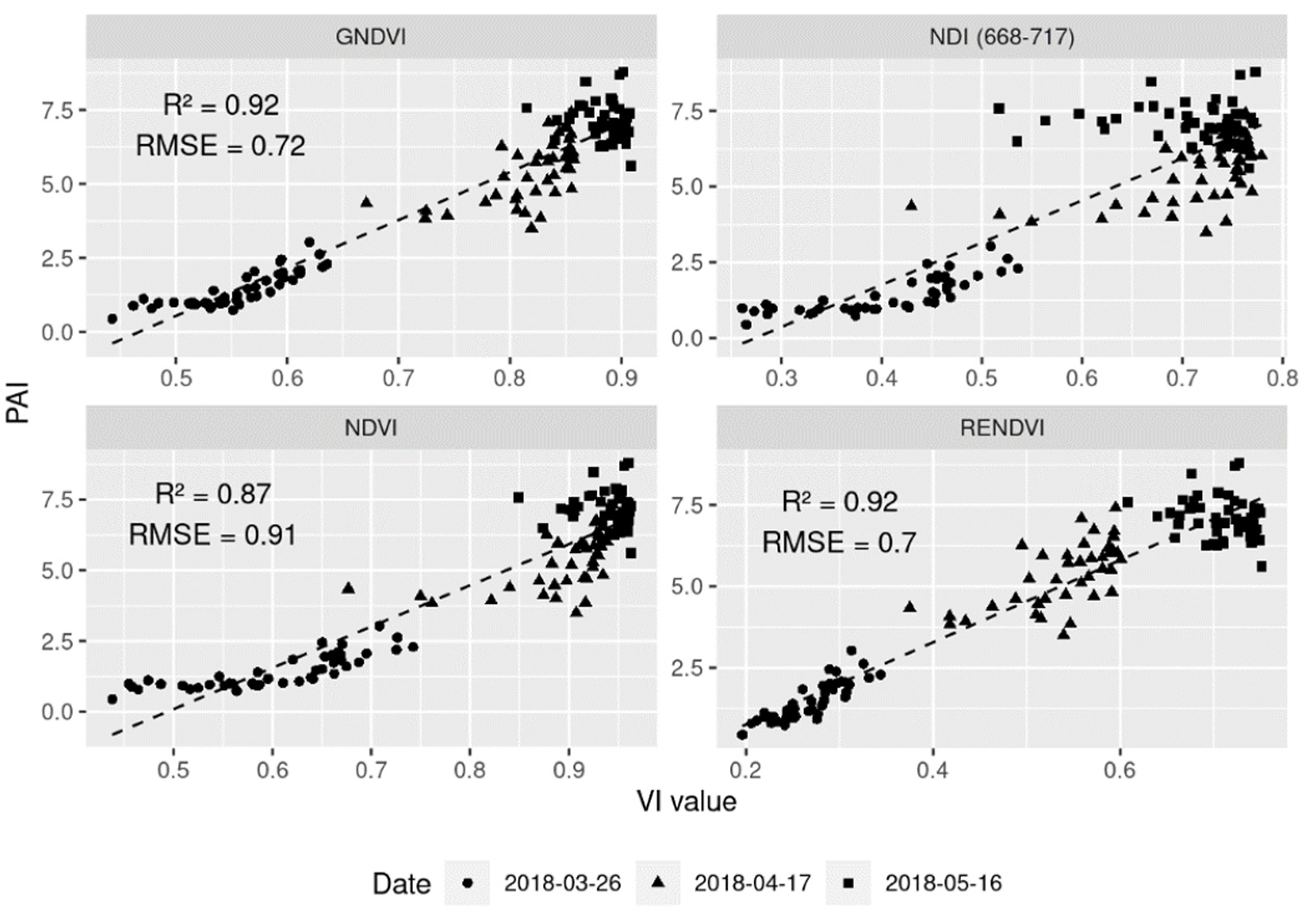
668-717 level off in April and May, and their values seem to no longer reflect the crop growth and development of winter wheat (Figure 5 and Figure 6). Among the four VIs, RENDVI shows the smallest saturation effect in May. The linear regression of VI to PAI resulted in an R2 and an RMSE of, respectively, 0.92 and 0.72 for GNDVI, 0.92 and 0.7 for RENDVI, 0.87 and 0.91 for NDVI, and 0.77 and 1.2 for NDI668-717 (Figure 6). It should be noted that we used the VIs derived from the UAV sensor as a proxy for the crop growth in order to map its heterogeneity within the field. For such a proxy assessment against ground-truth PAI data, we assumed that a simple linear regression was sufficient and more straightforward than, for example, partial least square or RF regressions. Based on the goodness of fit of the regressions and the evolution of the VIs throughout the growing season (Figure 5), RENDVI was chosen as the best remotely sensed proxy for crop growth.

3.3.2. RENDVI and Final Yield Maps

RENDVI and yield maps present similar patterns throughout the growing season (Figure 7). The effects of the former field layout on the crop growth appear, with the northeastern (B) and southeastern (D) parcels showing higher biomass and yields.
The Spearman rank correlation coefficient (Sp), calculated for all combinations of RENDVI acquisition dates and yield (pixel scale), confirms the stability of the patterns in vegetation and yield throughout time. Sp is larger than 0.8 amongst RENDVI values at the three acquisition dates and larger than 0.7 between yield and RENDVI values at each acquisition date.
Additionally, RENDVI and yield maps are displayed, classified into five groups of the same number of pixels, defined by four quantiles (Figure 8). This allowed to highlight the time-continuity of intra-field heterogeneity along the growing season and at harvest. Moreover, this highlights more clearly the separation of the field into two main zones, defined quite well by the grouping of the A and C versus the B and D previous parcels, as it was defined by the analysis of historical management practices and soil samples. Nevertheless, these maps also show heterogeneity within each of the previous four parcels, which could be interesting to take into account in a field management variable zones approach.

3.4. Assessment of the Contribution of Soil Property Heterogeneity to In-Season Crop Growth and Final Yield Heterogeneity Using the CI-Forest Algorithm

The CI-forest models for the entire field performed very well at fitting: they explained variance of 66–87% (Figure 9).
The crop growth was best predicted by the CI-forest model at the beginning of the growing season. By the end of March, the model explained 87% of the observed variance. Model performances decreased over time, from 87% to 66%.
K and pH were identified as the most important and stable explanatory variables for crop growth throughout the entire growing season, explaining from 15% up to 26% of the variance in crop growth and yield each. The former field layout (OB variable) was amongst the top ranked for the crop growth throughout the growing season and for the yield, except for mid-May where SOC and DEM emerged as more important splitting variables for the prediction of crop growth. In contrast, Mn, Ca, clay, P, and Ntot were not important splitting variables either for crop growth or yield in any of the CI-forest models. Mg was marginally important at the beginning of the season (end-March) and at harvest (mid-July), but this instability might be attributed to the randomness of the model. These soil parameters did not generate any heterogeneity in crop growth, meaning that they were probably not the limiting growth factors.
Given the importance of the former field layout in all CI-forest models, we carried out the same CI-forest analysis for each of the four former parcels. The results are reported in the Appendix A (Figure A3). Overall, the model performance decreased for each parcel compared to the results from the entire field, with the highest R2 = 0.82 obtained for Parcel B in April, and the lowest R2 = 0.28 obtained for parcel A in July. The interpretation of the results must be performed with care as the models have, in some cases, very poor explanatory ability. The variable importance rankings for RENDVI and yield vary strongly amongst parcels. While in the CI-forest analysis for the whole field pH was the most discriminatory variable, this is only the case for parcel C in May. On the other hand, the second most discriminatory variable for the entire field, K, is top-ranked in parcels A and B during crop growth stages. This highlights once more the impact of the heritage of former field division and of historical soil and crop management practices. Moreover, each parcel presents instability throughout time, as explanatory variables are ranked differently in the CI-forest from March to July. Parcels A and C are witnessing this effect more noticeably.

4. Discussion

Characterizing the intra-field heterogeneity of crop growth is the first step for defining field management variable zones in precision agriculture. Several combinations of “NDI” [7] were tested to explore the possibilities of the UAV-borne MicaSense® RedEdge-MTM sensor to characterize the growth heterogeneity throughout the growing season. The combination of red-edge and red bands was the most suitable to show the continuity in winter wheat crop growth patterns, even at a late growing stage (mid-May). It performed better than the NDVI, classically used in precision agriculture applications [2] and showing saturation issues between stem elongation stage (mid-April) and flag leaf stage (mid-May) of winter wheat crop. Similar patterns have been observed between RENDVI maps and yield maps (Sp = 0.7), which led us to consider RENDVI maps to be a good predictor for final yield heterogeneity. As a comparison, Maestrini and Basso [5] showed an in-season correlation of maximum 0.5 between wheat final yield and NDVI and considered it as a good predictor for yield heterogeneity. This confirms the potential of RENDVI maps to characterize the winter wheat crop growth and yield.
OK is known to be a robust method to produce soil properties maps for agricultural applications [22,23,24]. Our study confirmed its robustness considering the small relative RMSECV obtained for kriged soil property maps (maximum 0.24).
CI-forest models showed the strong influence of soil properties heterogeneity on crop growth heterogeneity. This link is stronger early in the season (March) and decreases until harvest, potentially illustrating an increasing effect of intra-annual variability on the heterogeneity of the crop growth. According to the variable importance analysis, DEM and SOC importance raised in mid-May. Topography is closely related to concentration of runoff at the footslopes. A positive correlation has been found between soil wetness and SOC in numerous studies [33,34,35]. Between the 17 April 2018 and 15 May 2018 UAV flights (28 days), there was a total of 49.5 mm precipitation, 33.1 and 12.4 mm of which fell in 2 consecutive days at the end of April (Figure 2). Hence, this period was quite dry and the heavy rain storms have probably led to concentration of runoff and higher moisture contents in the soils of the lower part of the field. We therefore hypothesize that the crop growth at the end of the growing season was faster where more soil moisture was available.
According to the CI-forest variable importance analysis, the soil properties related to the most crop growth and yield heterogeneity were K and pH and, to a lower extent, SOC and Mg. In this study case, they can therefore be considered as limiting factors for the crop growth and final yield on at least part of the field and we can analyze whether these are parameters that should be taken into account primarily in such a field to apply a management zones approach. In the conditions of the silty soils of the Belgian loam belt and ideal crop growing conditions, Van Koninckxloo and Brassart [36] described optimal values for the abovementioned soil properties as follows: pH = 6.9; K = 16 mg/100 g; Mg = 12 mg/100 g; SOC = 1.25 g/100 g. Keeping in mind that soil was sampled after the harvest of winter wheat crop, which received no input other than nitrogen and has a low demand for other nutrients, it is interesting to compare such values with our data and results from the CI-forest analysis. Considering firstly the average values over the whole field area, pH values ranging from 6.9 to 7.9 can be qualified as alkaline values higher than the optimal. However, according to Fernandez and Hoeft [37], such basic pH values are still adequate for winter wheat crop growth. K values ranging from 13.8 to 34.7 mg/100 g are close to or higher than the optimal value. SOC values ranging from 0.8 to 1.5% are mainly lower than the optimal ones. Mg values ranging from 5 to 14.7 mg/100 g are also generally too low compared to optimal values. For the four soil properties identified in our study as linked to the winter wheat crop growth and final yield heterogeneity, such value range fluctuations with raw values are quite distant from the expected optimal ones, indicating the potential to discriminate management variable zones within the field, based on the use of UAV-embedded multispectral sensor and RENDVI image acquisition. Considering the crop growth and final yield heterogeneity over the four previous parcels from the former field layout, parcels B and D clearly indicate higher crop growth and yield values compared to parcels A and C (Figure 7). Similarly, mean values of variables pH, K, and SOC were also significantly higher within B and D parcels, while Mg showed significantly higher value in parcel D only. Considering pH and K factors, as stated above, it is not known from the literature that increasing values of both factors, per se, has increasing effect on winter wheat crop growth and yield, but it could be argued that the interaction of both can explain differences in crop growth and yield. Indeed, as mentioned before, pH values are quite alkaline and could partially reduce the availability and plant assimilation of K in this value range [38], but pH limitation is probably not the only explanation, because, as stated by IPNI [39], availability and uptake of K is often complicated by many interacting components such as soil and plant characteristics and also fertilizer and management practices. For soil, one can mention, for instance, its cation exchange capacity, the amount of available K in the soil solution, the K fixation of the soil, or the nonexchangeable or slowly available K. K is also known to interact with almost all of the essential macronutrients, secondary nutrients, and micronutrients, so that crop growth and yield can be affected. As K amount in B and D parcels are higher, this limitation could be mitigated so that induced deficiency effect of K on crop growth and yield is much lower or even avoided in both B and D situations. On the contrary, a direct effect of higher SOC values in B and D parcels can explain increase in crop growth and yield. This is supported by a global meta-analysis conducted by Oldfield et al. [40], showing that winter wheat yield increases with SOC until it levels off at SOC contents of 2%. This can be explained through the soil biological activity that increases with higher SOC content. Finally, the effect of Mg soil content is to be related to K effect as both nutrients show quite similar behavior in the soil–plant relationship. From this analysis, it is important to conclude that not only the single effect of limiting or boosting factors on crop growth but also their complex interactions need to be taken into account.
The analyses and discussion in the previous paragraph illustrate the link that is established in our case study between crop growth heterogeneity assessed through UAV spectral sensor and the observed and geolocalized heterogeneity in specific physical and chemical soil parameters, leading to the identification and localization of management variables zones within a field. We considered one growing season after the consolidation of four former fields two years earlier. The former fields were managed differently and this remarkably impacted the soil nutrients availability, the pH, and the SOC, as reflected by the historical management data analysis and the soil sampling analyses. This difference in historical management induced crop growth heterogeneity, as depicted by the crop growth maps. Management zones based only on the former field layout and the historical management, with the definition of two main zones: A–C and B–D former parcels, would already allow a good enhancement of organic and calcic amendments or fertilizers management. In our case study, crop growth spatial patterns are a strong indicator for the legacy of management on soil properties.
Given the observed strong link between some soil property heterogeneity and winter wheat crop growth, especially at the tillering stage, we can assume that it would be possible to describe the heterogeneity resulting from the combination of soil properties limiting crop growth on at least part of the field from an early-season crop growth map. In our case, the heterogeneity of the crop growth at tillering is representative of the heterogeneity of pH and K, themselves strongly correlated to the former field management and layout. As these crop growth patterns are related to soil properties, the patterns can therefore be useful for the identification of soil sampling areas. Taking enough soil samples to characterize the heterogeneity of the field is essential to achieve an optimal site-specific management. Such an operation completed for this study is labor-intensive and represents a significant cost (approximately 25 euro per sample) for the farmer, but these data can allow the farmer to save inputs by applying a management zones approach for several years on its field. This sampling must be carried out at the most relevant locations to properly characterize the heterogeneity of a field while optimizing the number of samples required and therefore the cost of the operation. The analysis of winter wheat crop growth, especially at the beginning of the growing season, near the tillering stage, allows a characterization of soil-induced heterogeneity by dividing the field into zones that could be taken into consideration to target soil analyses and then be used as management zones. Soil analysis remains important and can be completed or replaced by remote sensing of bare soil to create objective maps of soil properties, such as SOC [41], or textural properties [42].

5. Conclusions

In precision agriculture, a good assessment of the crop heterogeneity throughout the growing season is essential as a first step to understand and predict yield heterogeneity. We have shown that it can be performed efficiently by RENDVI maps derived from a UAV-borne multispectral sensor. Analyzing and quantifying physical and chemical soil properties and their spatial variation within a field is essential to complete the assessment of crop growth by matching both information. Considering field management history is also very useful to this end. We have demonstrated the usefulness of the CI-forest technique for quantifying the importance of spatial variation in some soil properties heterogeneity on crop growth heterogeneity and suggested the link between. Our case study shows that such relevant assumptions between crop and soil can be used to reach a better management of organic and calcic amendments or fertilizers inputs by stressing the most relevant soil parameters to take into account in site-specific management. However, the analysis of the causal effect of soil properties on in-season crop growth and final yield illustrate that to identify a relevant action for inputs modulation, not only will the single effect of soil factors need to be considered, but also their interaction. It illustrates clearly that in such analysis, at least agronomy and plant/crop physiology concerns need to be merged for relevant decision in soil- and crop-adapted management practices aiming to efficiently mitigate soil heterogeneity within a field based on a management variable zones approach. In this way, this study indicates the strong link between spatial variation in soil properties and winter wheat crop growth and suggests that early season crop maps could be sufficient to define field management zones linked to spatial variation in soil properties.

Author Contributions

Conceptualization, D.G., K.D., Y.C., F.C., V.P., J.-P.G., and B.v.W.; methodology, D.G., K.D., G.C., Y.C., K.V.O., F.C., V.P., J.-P.G., and B.v.W.; software, D.G., K.D., G.C., K.V.O., and F.C.; formal analysis, D.G. and K.D.; investigation, D.G., G.C., Y.C., Q.L., and K.V.O.; resources, Q.L., K.V.O., V.P., and B.v.W.; data curation, D.G., G.C., and Q.L.; writing—original draft preparation, D.G. and K.D.; writing—review and editing, D.G., K.D., Y.C., V.P., J.-P.G., and B.v.W.; visualization, D.G. and K.D.; supervision, Y.C., V.P., J.-P.G., and B.v.W.; project administration, V.P. and B.v.W.; funding acquisition, Y.C., V.P., J.-P.G., and B.v.W. All authors have read and agreed to the published version of the manuscript.

Funding

This work was supported by the Research Programme for Earth Observation (STEREO III) of the Federal Science Policy (BELSPO under Grant SR/00/362—UAVSoil).

Data Availability Statement

Data are stored on Walloon Agricultural Research Center (CRA-W) servers and can be made available on demand through specific agreement. R code used for the data processing, analysis, and figure production is a custom code written for the only purpose of this paper.

Acknowledgments

Many thanks to Amaury Leclef who contributed to the field work, to Henri Michels who helped to find and gather the historical field management data, and to Belgian Scientific Policy (BELSPO) for the funding of this work. R (R Core Team 2018) was used for the data processing. Many thanks to the whole team and community for developing such a powerful and versatile tool.

Conflicts of Interest

The authors have no conflict of interest to declare that are relevant to the content of this article.

Appendix A

Figure A1. Distribution frequency of the physical and chemical soil parameters (80 soil samples) over the whole studied field in 2018.
Remotesensing 14 02806 g0a1
Figure A2. Boxplots of the soil parameters (samples) for the four previous parcels (A, B, C, and D) of the former field layout (see Figure 1). The p-value significance code resulting from ANOVA test for each variable and between the four previous fields is indicated after the variable name. Significance code : *** = 0 to 0.001 p-value; ** = 0.001 to 0.01; * = 0.01 to 0.05 ; . = 0.05 to 0.1.
Remotesensing 14 02806 g0a2
Figure A3. Relative variable importance (RVI) of predictor variables (variable importance of a given variable normalized to the sum of variable importance of all variables in the model) influential to crop growth at four dates during the growing season of the winter wheat crop in 2018 for each of the four former parcels (AD) of the former field layout (see Figure 1), calculated by conditional inference forest algorithm after the removal of correlated variables. The vertical dashed line indicates the expected importance in a completely random model. The performance of the models was evaluated using the R2 and RMSE throughout the winter wheat growing season and the harvest. * Expressed in kg ha−1.
Remotesensing 14 02806 g0a3

References

  1. Alexandratos, N.; Bruinsma, J. World Agriculture towards 2030/2050: The 2012 Revision; ESA Working Papers 12-03; FAO: Rome, Italy, 2012. [Google Scholar]
  2. Mulla, D.J. Twenty Five Years of Remote Sensing in Precision Agriculture: Key Advances and Remaining Knowledge Gaps. Biosyst. Eng. 2013, 114, 358–371. [Google Scholar] [CrossRef]
  3. Awika, J.M. Major Cereal Grains Production and Use around the World. In Advances in Cereal Science: Implications to Food Processing and Health Promotion; Awika, J.M., Piironen, V., Bean, S., Eds.; American Chemical Society: Washington, DC, USA, 2011; Volume 1089, pp. 1–13. ISBN 978-0-8412-2636-4. [Google Scholar]
  4. Gebbers, R.; Adamchuk, V.I. Precision Agriculture and Food Security. Science 2010, 327, 828–831. [Google Scholar] [CrossRef] [PubMed]
  5. Maestrini, B.; Basso, B. Predicting Spatial Patterns of Within-Field Crop Yield Variability. Field Crops Res. 2018, 219, 106–112. [Google Scholar] [CrossRef]
  6. Lauzon, J.D.; Fallow, D.J.; O’Halloran, I.P.; Gregory, S.D.L.; von Bertoldi, A.P. Assessing the Temporal Stability of Spatial Patterns in Crop Yields Using Combine Yield Monitor Data. Can. J. Soil Sci. 2005, 85, 439–451. [Google Scholar] [CrossRef]
  7. Delegido, J.; Verrelst, J.; Alonso, L.; Moreno, J. Evaluation of Sentinel-2 Red-Edge Bands for Empirical Estimation of Green LAI and Chlorophyll Content. Sensors 2011, 11, 7063–7081. [Google Scholar] [CrossRef] [PubMed] [Green Version]
  8. Whitehead, K.; Hugenholtz, C.H. Remote Sensing of the Environment with Small Unmanned Aircraft Systems (UASs), Part 1: A Review of Progress and Challenges. J. Unmanned Veh. Syst. 2014, 2, 69–85. [Google Scholar] [CrossRef]
  9. Lukas, V.; Novák, J.; Neudert, L.; Svobodova, I.; Rodriguez-Moreno, F.; Edrees, M.; Kren, J. The Combination of UAV Survey And Landsat Imagery for Monitoring of Crop Vigor in Precision Agriculture. ISPRS—Int. Arch. Photogramm. Remote Sens. Spat. Inf. Sci. 2016, XLI-B8, 953–957. [Google Scholar] [CrossRef] [Green Version]
  10. Schirrmann, M.; Giebel, A.; Gleiniger, F.; Pflanz, M.; Lentschke, J.; Dammer, K.-H. Monitoring Agronomic Parameters of Winter Wheat Crops with Low-Cost UAV Imagery. Remote Sens. 2016, 8, 706. [Google Scholar] [CrossRef] [Green Version]
  11. Bendig, J.; Yu, K.; Aasen, H.; Bolten, A.; Bennertz, S.; Broscheit, J.; Gnyp, M.L.; Bareth, G. Combining UAV-Based Plant Height from Crop Surface Models, Visible, and near Infrared Vegetation Indices for Biomass Monitoring in Barley. Int. J. Appl. Earth Obs. Geoinform. 2015, 39, 79–87. [Google Scholar] [CrossRef]
  12. COMIFER Teneurs En P, K et Mg Des Organes Végétaux Récoltés Pour Les Cultures de Plein Champ et Les Principaux Fourrages. Available online: https://comifer.asso.fr/fr/publications.html (accessed on 10 March 2022).
  13. Lakanen, E.; Erviö, R. A Comparison of Eight Extractants for the Determination of Plant Available Micronutrients in Soils. Acta Agralia Fennica 1971, 123, 223–232. [Google Scholar]
  14. Jonckheere, I.; Fleck, S.; Nackaerts, K.; Muys, B.; Coppin, P.; Weiss, M.; Baret, F. Review of Methods for in Situ Leaf Area Index Determination: Part I. Theories, Sensors and Hemispherical Photography. Agric. For. Meteorol. 2004, 121, 19–35. [Google Scholar] [CrossRef]
  15. Fang, H.; Baret, F.; Plummer, S.; Schaepman-Strub, G. An Overview of Global Leaf Area Index (LAI): Methods, Products, Validation, and Applications. Rev. Geophys. 2019, 57, 739–799. [Google Scholar] [CrossRef]
  16. Weiss, M.; Baret, F. CAN_EYE V6.4.91 User Manual; INRAE: Avignon, France, 2017; Available online: https://www6.paca.inrae.fr/can-eye/content/download/3052/30819/version/4/file/CAN_EYE_User_Manual.pdf (accessed on 10 March 2020).
  17. Darvishzadeh, R.; Skidmore, A.; Atzberger, C.; van wieren, S. Estimation of Vegetation LAI from Hyperspectral Reflectance Data: Effects of Soil Type and Plant Architecture. Int. J. Appl. Earth Obs. Geoinf. 2008, 10, 358–373. [Google Scholar] [CrossRef]
  18. Rouse, J.W.; Hass, R.H.; Schell, J.A.; Deering, D.W. Monitoring Vegetation Systems in the Great Plains with ERTS; NASA: Washington, DC, USA, 1974. [Google Scholar]
  19. Gitelson, A.A.; Kaufman, Y.J.; Merzlyak, M.N. Use of a Green Channel in Remote Sensing of Global Vegetation from EOS-MODIS. Remote Sens. Environ. 1996, 58, 289–298. [Google Scholar] [CrossRef]
  20. Gitelson, A.; Merzlyak, M.N. Quantitative Estimation of Chlorophyll-a Using Reflectance Spectra: Experiments with Autumn Chestnut and Maple Leaves. J. Photochem. Photobiol. B 1994, 22, 247–252. [Google Scholar] [CrossRef]
  21. Li, J.; Heap, A.D. Spatial Interpolation Methods Applied in the Environmental Sciences: A Review. Environ. Model. Softw. 2014, 53, 173–189. [Google Scholar] [CrossRef]
  22. Kravchenko, A.; Bullock, D.G. A Comparative Study of Interpolation Methods for Mapping Soil Properties. Agron. J. 1999, 91, 393–400. [Google Scholar] [CrossRef]
  23. Zhu, Q.; Lin, H.S. Comparing Ordinary Kriging and Regression Kriging for Soil Properties in Contrasting Landscapes. Pedosphere 2010, 20, 594–606. [Google Scholar] [CrossRef]
  24. Houlong, J.; Daibin, W.; Chen, X.; Shuduan, L.; Hongfeng, W.; Chao, Y.; Najia, L.; Yiyin, C.; Lina, G. Comparison of Kriging Interpolation Precision between Grid Sampling Scheme and Simple Random Sampling Scheme for Precision Agriculture. Eurasian J. Soil Sci. 2016, 5, 62–72. [Google Scholar] [CrossRef] [Green Version]
  25. López-Granados, F.; Jurado-Expósito, M.; Atenciano, S.; García-Ferrer, A.; Sánchez de la Orden, M.; García-Torres, L. Spatial Variability of Agricultural Soil Parameters in Southern Spain. Plant Soil 2002, 246, 97–105. [Google Scholar] [CrossRef]
  26. Williams, G. Random Forests. In Data Mining with Rattle and R: The Art of Excavating Data for Knowledge Discovery; Springer: New York, NY, USA, 2011; pp. 245–268. ISBN 978-1-4419-9890-3. [Google Scholar]
  27. Mascaro, J.; Asner, G.P.; Knapp, D.E.; Kennedy-Bowdoin, T.; Martin, R.E.; Anderson, C.; Higgins, M.; Chadwick, K.D. A Tale of Two “Forests”: Random Forest Machine Learning AIDS Tropical Forest Carbon Mapping. PLoS ONE 2014, 9, e85993. [Google Scholar] [CrossRef] [PubMed]
  28. Hobley, E.U.; Baldock, J.; Wilson, B. Environmental and Human Influences on Organic Carbon Fractions down the Soil Profile. Agric. Ecosyst. Environ. 2016, 223, 152–166. [Google Scholar] [CrossRef] [Green Version]
  29. Hobley, E.; Wilson, B.; Wilkie, A.; Gray, J.; Koen, T. Drivers of Soil Organic Carbon Storage and Vertical Distribution in Eastern Australia. Plant Soil 2015, 390, 111–127. [Google Scholar] [CrossRef]
  30. Strobl, C.; Boulesteix, A.-L.; Zeileis, A.; Hothorn, T. Bias in Random Forest Variable Importance Measures: Illustrations, Sources and a Solution. BMC Bioinform. 2007, 8, 25. [Google Scholar] [CrossRef] [Green Version]
  31. Chenu, C.; Angers, D.A.; Barré, P.; Derrien, D.; Arrouays, D.; Balesdent, J. Increasing Organic Stocks in Agricultural Soils: Knowledge Gaps and Potential Innovations. Soil Tillage Res. 2019, 188, 41–52. [Google Scholar] [CrossRef]
  32. B-CGMS Team Belgian Crop Growth Monitoring System (B-CGMS) 2018 Reports. Available online: http://b-cgms.cra.wallonie.be/ (accessed on 10 March 2022).
  33. Davidson, E.A. Spatial Covariation of Soil Organic Carbon, Clay Content, and Drainage Class at a Regional Scale. Landsc. Ecol. 1995, 10, 349–362. [Google Scholar] [CrossRef]
  34. Doetterl, S.; Stevens, A.; van Oost, K.; Quine, T.A.; van Wesemael, B. Spatially-Explicit Regional-Scale Prediction of Soil Organic Carbon Stocks in Cropland Using Environmental Variables and Mixed Model Approaches. Geoderma 2013, 204–205, 31–42. [Google Scholar] [CrossRef]
  35. Meersmans, J.; De Ridder, F.; Canters, F.; De Baets, S.; Van Molle, M. A Multiple Regression Approach to Assess the Spatial Distribution of Soil Organic Carbon (SOC) at the Regional Scale (Flanders, Belgium). Geoderma 2008, 143, 1–13. [Google Scholar] [CrossRef]
  36. Van Koninckxloo, M.; Brassart, D. 30 Ans d’agriculture En Hainaut 2020. Available online: http://www.carah.be/documents-telechargeables.html (accessed on 10 March 2022).
  37. Fernández, F.G.; Hoeft, R.G. Managing Soil PH and Crop Nutrients. In Illinois Agronomy Handbook; University of Illinois at Urbana Champaign: Champaign, IL, USA, 2009; p. 22. [Google Scholar]
  38. Truog, E. Lime in Relation to Availability of Plant Nutrients. Soil Sci. 1948, 65, 1–8. [Google Scholar] [CrossRef]
  39. International Plant Nutrition Institute (IPNI). Better Crops with Plant Food—Potassium for Agriculture. 1998, Volume 82. Available online: http://www.ipni.net/publication/bettercrops.nsf/0/E90E04A957EA624285257980007CD63C/$FILE/BC-1998-3.pdf (accessed on 10 March 2022).
  40. Oldfield, E.E.; Bradford, M.A.; Wood, S.A. Global Meta-Analysis of the Relationship between Soil Organic Matter and Crop Yields. Soil 2019, 5, 15–32. [Google Scholar] [CrossRef] [Green Version]
  41. Castaldi, F.; Hueni, A.; Chabrillat, S.; Ward, K.; Buttafuoco, G.; Bomans, B.; Vreys, K.; Brell, M.; van Wesemael, B. Evaluating the Capability of the Sentinel 2 Data for Soil Organic Carbon Prediction in Croplands. ISPRS J. Photogramm. Remote Sens. 2019, 147, 267–282. [Google Scholar] [CrossRef]
  42. Casa, R.; Castaldi, F.; Pascucci, S.; Pignatti, S. Potential of hyperspectral remote sensing for field scale soil mapping and precision agriculture applications. Ital. J. Agron. 2012, 7, 331–336. [Google Scholar] [CrossRef]
Figure 1. RGB image of the study site (Bing Aerial®). Dashed lines delineate the former field layout (parcels A, B, C, and D) before merging in spring 2017 to make up the 17 ha field. The black continuous line delineates the study area, defined by applying an inner buffer of 5 m, deleting the headlands and keeping only the common area between the three unmanned aerial vehicle (UAV) images captured during the 2018 winter wheat growing season. Dots indicate locations of soil samples and triangles indicate locations of plant area index (PAI) measurements (May 2018).
Remotesensing 14 02806 g001
Figure 2. Timeline from 1 January to 31 August 2018 of daily meteorological data (temperature, rainfall, cumulative rainfall), UAV flights occurrences, fertilizer N applications, harvest, and soil sampling over the experimental field of 17 ha located in Gembloux (Belgium) for the present study and cropped with winter wheat. First graph represents minimum, average (continuous line), and maximum temperature.
Remotesensing 14 02806 g002
Figure 3. Pearson correlation matrix of the soil parameters from the 80 topsoil samples collected on the study field in August 2018.
Remotesensing 14 02806 g003
Figure 4. Maps of interpolated soil variables by ordinary kriging and DEM map. Points represent the location of the topsoil sampling, and gray lines show the delineation of the previous four parcels (A, B, C, and D) of the former field layout which were merged in 2017 (see Figure 1). The black border delineates the study area which is used as input in the CI-forest algorithm.
Remotesensing 14 02806 g004
Figure 5. Temporal evolution of the VIs derived from spectral information acquired by MicaSense® RedEdge-MTM sensor embedded on a quadcopter UAV on three dates in 2018 over the studied field sown with winter wheat. NDI (668-717) = NDI668-717.
Remotesensing 14 02806 g005
Figure 6. VI values derived from spectral information acquired by MicaSense® RedEdge-MTM sensor mounted on quadcopter UAV plotted against ground-truth measurements of PAI derived from ground-truth digital hemispherical photography (DHP) during the 2018 winter wheat growing season (end March, mid-April, mid-May) over the studied field. NDI (668-717) = NDI668-717.
Remotesensing 14 02806 g006
Figure 7. RENDVI acquired by MicaSense® RedEdge-MTM sensor embedded on a quadcopter UAV and winter wheat grain yield (measured during the harvest on 17 July 2018 with a John Deere sensor) maps showing the crop growth heterogeneity and its continuity all along the considered growing period from March to July 2018. The gray lines illustrate the delineation of the previous four parcels A, B, C, and D (after suppression of headlands), which were merged into a unique field in spring 2017 (see Figure 1).
Remotesensing 14 02806 g007
Figure 8. Class maps of RENDVI and winter wheat grain yield (classified into five groups of the same number of pixels, defined by four quantiles). See Figure 7 for details on acquisition and historical former field layout.
Remotesensing 14 02806 g008
Figure 9. Relative variable importance (RVI) of predictor variables (variable importance of a given variable normalized to the sum of variable importance of all variables in the model) influential to crop growth and yields at four dates, during the growing season of winter wheat crop in 2018 over the study area (see Figure 1), calculated by CI-forest algorithm after the removal of correlated variables. The vertical dashed line indicates the expected importance in a completely random model. The performance of the models was evaluated using the R2 and the RMSE throughout the growing season and the harvest. * Expressed in kg ha−1. OB stands for old borders, of the former field layout into four parcels.
Remotesensing 14 02806 g009
Table 1. Soil properties monitored and methodology used for the samples analysis.
Soil Property(ies)MethodologyReference
PExtraction using ammonium acetate and ethylenediaminetetraacetic acid and analysis by injection flow colorimetry.[13]
K, Mg, Ca, Fe, Mn, NaExtraction using ammonium acetate and ethylenediaminetetraacetic acid and dosage by and analysis by flame atomic absorption spectrometry.[13]
pHGlass electrode in a suspension of soil diluted 1:5 (volume fraction) in a 1 mol·L−1 potassium chloride solution.NF ISO 10390
SOCDry combustion (DUMAS).Derived from NF ISO 10694
NDry combustion (DUMAS).Derived from NF ISO 13878
TextureSedimentation and sieving to determine the percentage of clay (particle size < 2µm), silt (particle size between 2 and 50 µm), and sand (particle size > 50 µm).Derived from NF X 31–107
Table 2. Specifications of the RedEdge-MTM sensor from MicaSense®.
Spectral BandCenter Wavelength (nm)Bandwidth (nm)
Blue (B)47520
Green (G)56020
Red (R)66810
Red edge (RE)71710
Near-IR (NIR)84040
Table 3. Vegetation indices (VIs) computed using spectral data from the RedEdge-MTM camera spectral sensor embedded on a quadcopter-type UAV (a DJI Phantom 3 and a custom-made model with DJI N3 controller).
Vegetation IndexAbbreviationFormulaReference
Normalized Difference Vegetation IndexNDVINIR − R/NIR + R[18]
Green NDVIGNDVINIR − G/NIR + G[19]
Red-Edge NDVIRENDVINIR − RE/NIR + RE[20]
Normalized Difference IndexNDI668-717RE − R/RE + R[7]
Table 4. Summary of historical soil and crop management practices data related to organic matter restitution or application in each of the four parcels (A, B, C, and D) of the former field layout (see Figure 1). Annual data are summed for four periods (2014–2018, 2010–2018, 2000–2018, 1990–2018). # = Number of occurrences. Residues = crop residues restitution.
PeriodParcelWinter Cover CropResiduesFarmyard ManureSlurryWaste Lime
#Type(s)##t·ha−1#m3·ha−1#t·ha−1
2014–2018A2mixture0000000
B1mixture3000000
C2mixture2000000
D2mixture10014000
2010–2018A3raygrass, mixture30013000
B2raygrass, mixture427026000
C2mixture2000000
D3mixture227014000
2000–2018A5mustard, raygrass, mixture7275130237
B3mustard, raygrass, mixture75165260115
C3mustard, mixture813500115
D4mustard, mixture105170140115
1990–2018A5mustard, raygrass, mixture103100130359
B4mustard, raygrass, mixture117220260240
C4mustard, mixture1138500375
D4mustard, mixture157270140115
Table 5. Summary of historical P, K, Mg, and Ca nutrient import and export in each of the four parcels (A, B, C, and D) of the former field layout (see Figure 1). Annual data are summed for four periods (2014–2018, 2010–2018, 2000–2018, 1990–2018). Organic imports (OI) refers to farmyard manure, slurry, and waste lime, as stated in Table 4. Mineral imports (MI) refers to various mineral amendments or fertilizers. Imports (Imp) is the sum of OI and MI. Exports (Exp) of P, K, and Mg are based on crop-yield-based estimation uptake at harvest from COMIFER references tables [12]. Dif is the difference between Exp and Imp.
PeriodParcelP2O5 (kg·ha−1)K2O (kg·ha−1)MgO (kg·ha−1)CaO (kg·ha−1)
OIMIImpExpDifOIMIImpExpDifOIMIImpExpDifOIMIImp
2014–2018A0120120465−34502502501128−878000176−1760150150
B03030263−23303030403−37300075−750150150
C0120120316−1960250250748−498000118−118000
D7230102337−23516030190812-62240040134−9480080
2010–2018A54120174559−3851202503701234−86430030181−15160150210
B4303046033812287030900542358200020096104554150704
C0200200504−30405305301025−495000164−164000
D4081105185031582531011351154−191800180196−166470647
2000–2018A73243611681089798691490236022649645804583768216353952030
B100211011127883241755710246515079585026001102251851159310552648
C296410706726−203451400174514453001820182228−46667180847
D10031901193912281175599027451924821492049232217017171601877
1990–2018A104543614811710−2291138149026283763−113567206725997324503952845
B14801401620140022023001760406032987628006001400464936268410553739
C106641014761217259915260035152518997732073241032227771802957
D146319016531446207265599036453129516692069254015223371602497
Table 6. Averaged, minimum, and maximal values of soil properties over the whole experimental field of 17 ha. The last column shows the conventional significance code of p-value (p-V SC) of an analysis of variance (ANOVA) test for four groups of soil samples partitioned based on their location within the four parcels (A, B, C, and D) of the former field layout (see Figure 1). CV = coefficient of variation. Significance code : *** = 0 to 0.001 p-value; ** = 0.001 to 0.01; * = 0.01 to 0.05; . = 0.05 to 0.1.
VariableUnitMinMaxMeanSDCV (%)p-V SC
Clay%12.422.3182.413.
Camg/100 g223.7803339.384.725*
Femg/kg241.7593346.783.424***
Kmg/100 g13.934.721.73.617***
Mgmg/100 g514.79.21.819**
Mnmg/kg187.7317.6231.23314**
Namg/100 g0.44.21.90.842.
Ntot%0.10.10.10.017.
Pmg/100 g7.225.512.33.831*
pH/6.97.97.60.33***
Sand%5.411.46.70.812
Silt%71.28075.423.
SOCg/kg8.31510.31.313***
Table 7. Ordinary kriging parameters for the soil variables selected as input for the final conditional inference forest (CI-forest) algorithm. RMSECV = RMSE of cross validation, rRMSCVE = relative RMSECV.
VariableNuggetSillRange (m)Nugget/SillRMSECVrRMSECV
P0.9913.38134.770.072.950.24
K3.999.89237.240.42.840.13
Mg1.12.27160.190.481.520.17
Ca2161.696816.59367.590.3265.40.19
pH (KCl)0.40.574531.110.70.190.02
Mn01191.92124.910250.11
SOC0.7718.617525.210.041.060.1
Ntot0092.990.510.010.07
clay05.99121.8901.850.1
Publisher’s Note: MDPI stays neutral with regard to jurisdictional claims in published maps and institutional affiliations.

