Article

Triplet-Metric-Guided Multi-Scale Attention for Remote Sensing Image Scene Classification with a Convolutional Neural Network

1
Key Laboratory of Photoelectronic Imaging Technology and System, Ministry of Education of China, Beijing Institute of Technology, Beijing 100081, China
2
School of Optics and Photonics, Beijing Institute of Technology, Beijing 100081, China
*
Author to whom correspondence should be addressed.
Remote Sens. 2022, 14(12), 2794; https://doi.org/10.3390/rs14122794
Submission received: 23 April 2022 / Revised: 1 June 2022 / Accepted: 8 June 2022 / Published: 10 June 2022

Abstract

:
Remote sensing image scene classification (RSISC) plays a vital role in remote sensing applications. Recent methods based on convolutional neural networks (CNNs) have driven the development of RSISC. However, these approaches are not adequate considering the contributions of different features to the global decision. In this paper, triplet-metric-guided multi-scale attention (TMGMA) is proposed to enhance task-related salient features and suppress task-unrelated salient and redundant features. Firstly, we design the multi-scale attention module (MAM) guided by multi-scale feature maps to adaptively emphasize salient features and simultaneously fuse multi-scale and contextual information. Secondly, to capture task-related salient features, we use the triplet metric (TM) to optimize the learning of MAM under the constraint that the distance of the negative pair is supposed to be larger than the distance of the positive pair. Notably, the MAM and TM collaboration can enforce learning a more discriminative model. As such, our TMGMA can avoid the classification confusion caused by only using the attention mechanism and the excessive correction of features caused by only using the metric learning. Extensive experiments demonstrate that our TMGMA outperforms the ResNet50 baseline by 0.47% on the UC Merced, 1.46% on the AID, and 1.55% on the NWPU-RESISC45 dataset, respectively, and achieves performance that is competitive with other state-of-the-art methods.

1. Introduction

Remote sensing image scene classification (RSISC), which is defined as a process of classifying remote sensing images into a discrete set of categories, may have broad applications in land-use surveying [1,2], urban planning [3], natural hazard detection [4,5], geographic image retrieval [6,7], and so on. Over the past few decades, RSISC has been a hot research focus, and some gratifying results [8,9,10,11,12] have been achieved. However, RSISC still faces challenges in:
  • Large diversity within classes: some scenes in the same class can be very different. As shown in Figure 1, in the first row, four scenes of the palace are different in appearance, shape, color, etc..
  • High similarity between classes: some scenes from different categories express similar geographical features. From the second row of Figure 1, we can see that the forest and sparse residential (freeway and runway) areas have strong similarities, such as spatial distribution, appearance, and texture.
  • The large variance of object/scene scales: when collecting remote sensing images, the scale of object/scene can change arbitrarily due to the different ground sample distances. In the third row of Figure 1, from airplane01 to airplane02, and from storage tank01 to storage tank02, there are large spatial scale variations.
  • Coexistence of multi-class objects: there may be multiple different objects in a scene. For example, the basketball court and tennis court, listed in the last row of Figure 1, also have buildings and trees, alongside being semantically related regions.
In early literature, researchers used handcrafted features for RSISC, such as scale-invariant feature transform (SIFT) [13], local binary pattern (LBP) [14,15], and histogram of oriented gradients (HOG) [16]. Later, some methods encoded handcrafted features to generate unsupervised features, including k-means clustering, sparse coding [17], principal component analysis (PCA) [18], autoencoder [19], and bag of words (BoW) [4,8,20,21]. However, these features cannot convey abstract semantic information, so they are not suitable for remote sensing scenes.
Recently, since the convolutional neural network (CNN) can automatically extract high-level features from raw images, it was applied to RSISC and made remarkable progress [6,22,23,24,25,26,27,28,29,30,31]. For example, to adapt to object scale variations, a multi-scale CNN (MCNN) framework [32] was built for extracting scale-invariant features from multi-scale input. Some researchers [10,33,34] used the covariance matrix calculated from stacked multi-scale feature maps or multi-granularity regional images to automatically capture second-order statistics features. Researches have shown that appropriate fusing of local and global features can help to discover more discriminative semantics for remote sensing scenes [6,35,36]. In [37], the authors focused on constructing a robust space–frequency joint representation (RSFJR) for RSISC. In addition, Qi et al. [38] proposed a deep Siamese convolutional network with rotation invariance regularization to reduce the over-fitting. Zhang et al. [23] designed a more efficient search framework, RS-DARTS, to find the optimal network architecture. In general, these methods improve the discriminative ability of feature representation by mining multiple features and designing effective networks.
However, the aforementioned CNN-based approaches neglect the problem of redundant features, such as irrelevant semantics and noise. To consider the contributions of different features, some methods employed the attention mechanism [39,40,41,42,43,44] to involve salient features through the relevant excitation and irrelevant inhibition. For example, Wang et al. [31] used deformable convolution to extract features and spatial-channel attention to enhance the extracted features. Li et al. [45] proposed a gated recurrent multiattention neural network (GRMA-Net) to focus on informative regions at multiple stages in a network. Shi et al. [46] designed an attention-based multi-branch feature fusion CNN (AMB-CNN). The AMB-CNN consists of eight groups. The squeeze and excitation (SE) [40] module is used for the first three groups and the convolutional block attention module (CBAM) [44] is used for four to seven groups. Tang et al. [47] designed a parallel channel and spatial attention module to fully capture the local-level information and develop an attention consistent model to unify the attention areas of the image pairs with different angles. These methods do emphasize salient features in the input feature map, but (1) salient features are not all helpful for classification [27], and some may even cause classification confusion; (2) the attention is derived from single-scale feature maps, so these methods cannot effectively mine multi-scale information; and (3) the attention only focuses on the local-level information and fails to exploit the contextual information. Some methods combine metric learning [48,49,50] to constrain features through finding an appropriate similarity measurement between pairs of features and preserving desired distance structure. For example, Cheng et al. [11] designed a discriminative CNN (D-CNN) where the contrastive loss is used to guide the network to map paired images in the same class as closely as possible; otherwise, the opposite occurs. Zhang et al. [51] trained a CNN with multi-size input images and triplet loss. In the inference stage, triplet loss is performed on triplet data to raise inter-class diversity and intra-class similarity under the constraint that the negative pair distance is larger than the positive pair distance plus some margin. These methods do effectively boost the performance of scene classification. However, directly combining metric learning to constrain features to follow a distance criterion may cause excessive correction of features.
Taking the problems mentioned above into account, a qualified CNN-based solution for RSISC needs to be capable of discriminative feature representation, multi-scale representation, and preserving contextual information to boost the classification performance.
In this paper, we propose a novel RSISC method named triplet-metric-guided multi-scale attention (TMGMA) to enhance task-related salient features and suppress task-unrelated salient and redundant features. Our contributions are summarized as follows:
  • We propose a multi-scale attention module (MAM) for RSISC. It can emphasize salient features from multi-scale convolutional activation features and capture the contextual information.
  • We add triplet metric (TM) regularization in the objective function. It optimizes the learning of MAM and guides the MAM to pay attention to task-related salient features by constraining the distance of positive pairs to be smaller than negative pairs.
  • We make MAM and TM collaborate. This strategy allows for the better determination of the contribution of different features in global decision and enforces learning a more discriminative classification model.
  • We conducted extensive experiments on UC Merced [8], AID [52], and NWPU-RESISC45 [3] datasets and demonstrate that the TMGMA improves the performance of RSISC.
The rest of this paper is organized as follows. Section 2 details the architecture of the proposed TMGMA. In Section 3 and Section 4, experiments and analyses are presented, and visualizations (Grad-CAM and t-SNE) are used to show the effectiveness of the proposed method. Section 5 concludes this paper.

2. Materials and Methods

CNN-based methods have achieved considerable progress in RSISC. However, they do not adequately consider the contributions of different features to the global decision. Directly combining the attention mechanism or metric learning to capture salient features may cause classification confusion or excessive correction of features. Therefore, learning how to enhance task-related salient features is essential.
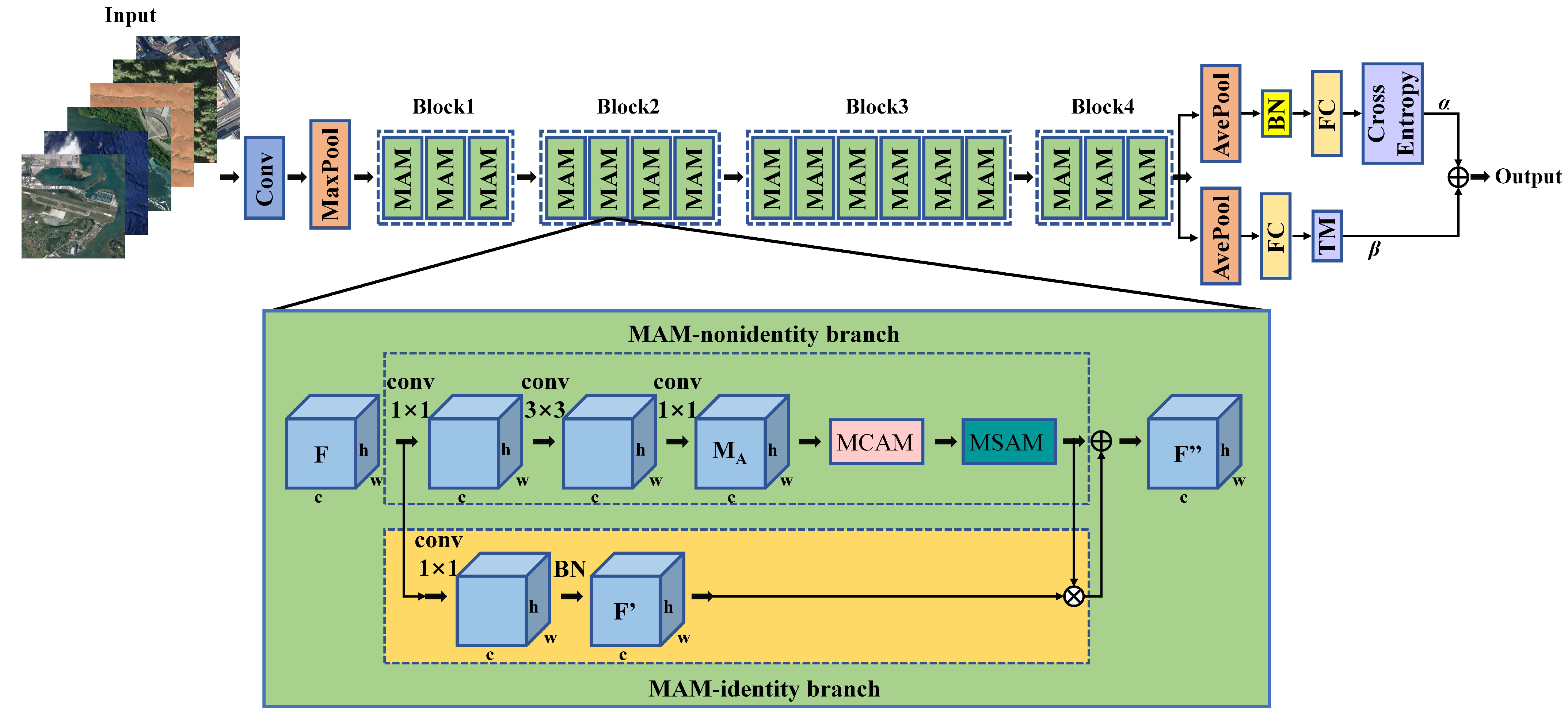
In our work, we propose a novel TMGMA to enhance task-related salient features and suppress task-unrelated salient and redundant features. We employed a widely-used CNN architecture, ResNet50 [53], as the basic network . As we know, each bottleneck of the ResNet50 backbone consists of identity and non-identity branches. In each bottleneck, following the non-identity branch, a multi-scale channel attention module (MCAM) and a multi-scale spatial attention module (MSAM) are added in series to perform channel- and spatial-wise attention from multi-scale feature maps, respectively. Moreover, the obtained multi-scale attention feature map is used as a weight map of the identity branch and refines its output. After that, two branches are summed element-wise to form the multi-scale attention module (MAM). In the objective function, a triplet metric (TM) regularization is added to optimize the learning of MAM. Figure 2 shows the overall structure.

2.1. Multi-Scale Channel Attention Module (MCAM)

In CNN, for an input image or feature map, CNN filters play the role of pattern detectors, and the output feature map in each channel is a response of the corresponding filter. Therefore, channel-wise, applying the attention mechanism can be seen as semantic attribute selection. Through channel-wise attention, the relevant semantic attributes are enhanced and the irrelevant are suppressed. A common problem with remote sensing images is that the scale of the object/scene can vary greatly depending on the earth’s observation distance. According to this, the multi-scale channel attention module (MCAM) is proposed. First, we perform channel dimension compression on the input feature map to reduce the computational burden. Second, convolution operations with differently sized kernels are executed in parallel, and the obtained multi-scale feature maps are chained together with the compressed input. Taking the concatenated feature maps can be helpful in the exploration of multi-scale information and effectively mine contextual information from adjacent scale feature maps. Third, global average pooling computes spatial statistics, which are further transmitted into a multi-layer perception (MLP) with one hidden layer. After that, a sigmoid activation function is utilized for re-calibration. Finally, the obtained channel-wise attention vector rectifies the input feature map.
As shown in Figure 3,the input feature map M A R C × H × W is first mapped into M B 0 with the size of C 4 × H × W using 1 × 1 convolution. Second, we conduct three transformations, each consisting of convolution, batch normalization (BN) [54], and ReLU [55], with kernel sizes 3 × 3 , 5 × 5 , and 7 × 7 , respectively. The outputs M B 1 , M B 2 , and M B 3 are C 4 × H × W in size, and they are concatenated together with M B 0 to flow multi-scale information into the next layer. Then, global average pooling aggregates the spatial information into a C × 1 vector, which is then delivered into MLP. Finally, element-wise multiplication is performed between the channel-wise attention vector and the input feature map M A R C × H × W to obtain the multi-scale channel attention feature map M C R C × H × W .
The calculation formulas of MCAM are as follows:
M B 0 = C o n v 1 × 1 ( M A ) ,
M B i = C o n v k i × k i ( M B 0 ) , i = 1 , 2 , 3
M B = C a t ( [ M B 0 , M B 1 , M B 2 , M B 3 ] ) ,
M C = σ ( M L P ( A v g P o o l ( M B ) ) ) M A = σ ( W 1 ( W 0 A v g P o o l ( M B ) + b 0 ) + b 1 ) M A ,
where k i = 2 × i + 1 , ⨂ represents element-wise multiplication, and σ denotes the sigmoid function. Note that, in Equation (1), W 0 R C τ × C , b 0 R C τ , W 1 R C × C τ , b 0 R C , and τ is a reduction factor used to decrease parameters in MLP.

2.2. Multi-Scale Spatial Attention Module (MSAM)

In MCAM, the concatenated feature maps are directly squeezed in spatial dimensions, and no spatial-wise attention is used. In general, to accurately recognize an image, we need to focally address the image foreground and inhibit the background interference. Considering each image region equally may cause sub-optimal classification results. Thus, spatial-wise attention needs to be added to emphasize important semantic regions. Hence, we propose the multi-scale spatial attention module (MSAM) to analyze the contributions over different semantic regions and capture contextual information through multi-scale feature maps. For the input feature map, we first apply several convolution operations to summarize channel dimension features in a multi-scale way. Then, the obtained multi-scale feature maps are spliced together in sequence. Finally, convolution is subsequently applied to learn the spatial-wise attention map which is used to refine the input feature map.
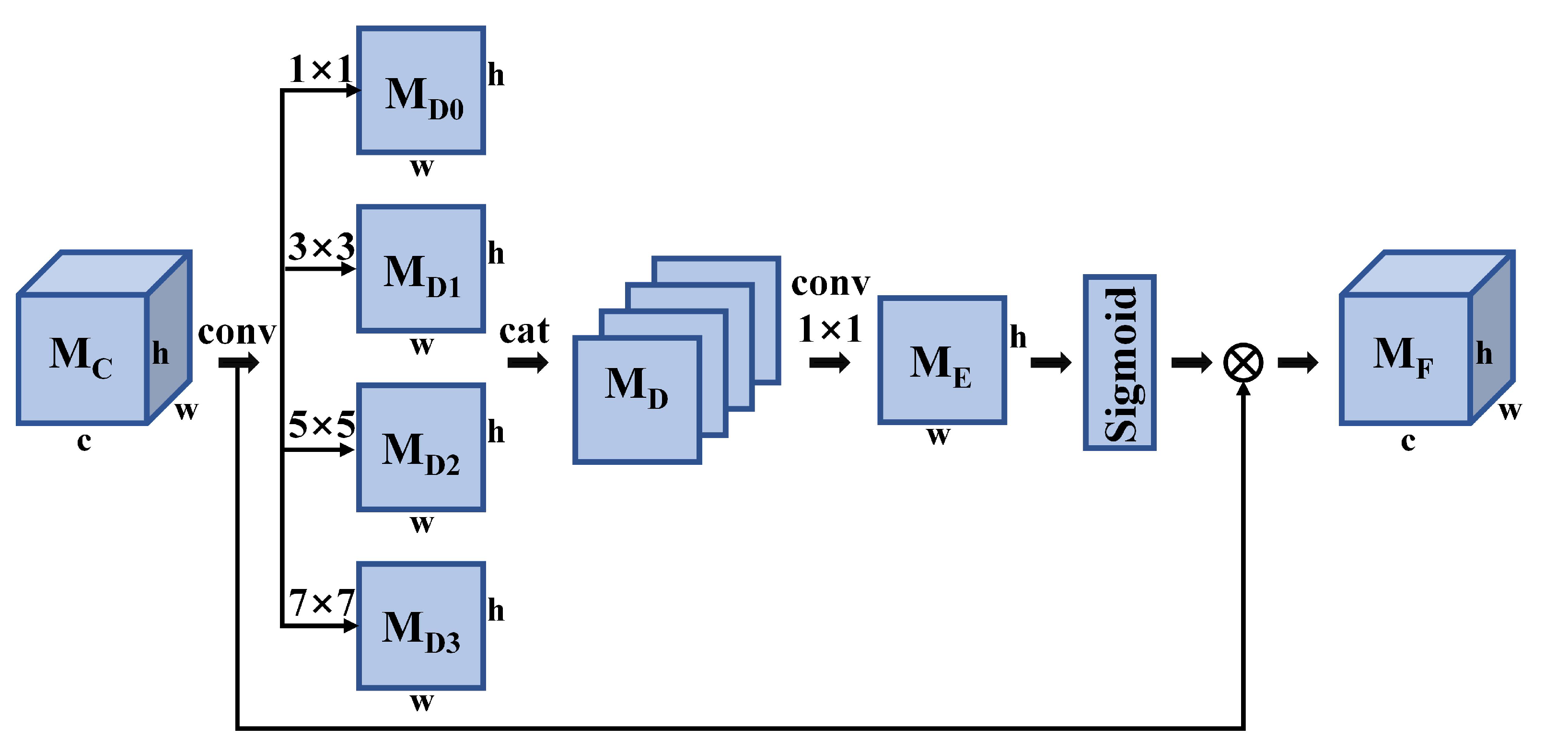
As shown in Figure 4, four convolution operations with 1 × 1 , 3 × 3 , 5 × 5 , and 7 × 7 convolution kernels are used on the multi-scale channel attention feature map M C R C × H × W . Based on this, the M C is converted into several feature maps, i.e., M D 0 R 1 × H × W , M D 1 R 1 × H × W , M D 2 R 1 × H × W , and M D 3 R 1 × H × W . Series connection is performed to obtain M D R 4 × H × W . Then, using a 1 × 1 convolution, the M D is mapped as a spatial-wise attention map M E R H × W . Finally, a multi-scale attention feature map M F R C × H × W is computed by multiplying M E and M C in an element-wise manner.
The MSAM is obtained by:
M D i = C o n v k i × k i ( M C ) , i = 0 , 1 , 2 , 3
M D = C a t ( [ M D 0 , M D 1 , M D 2 , M D 3 ] ) ,
M F = σ ( C o n v 1 × 1 ( M D ) ) M C ,
where C o n v k i × k i represents a series of operations of k i × k i convolution, BN, and ReLU. For simplicity, they are collectively called convolution operation. k i = 2 × i + 1 . σ is a sigmoid function used for normalization, and ⨂ indicates element-wise multiplication.

2.3. Multi-Scale Attention Module (MAM)

This section give a general description of the multi-scale attention module (MAM) in two parts: the MAM-nonidentity branch and the MAM-identity branch.
MAM-nonidentity branch: As shown in Figure 2, MCAM and MSAM are connected in series to construct this branch. The MCAM assesses the importance of the pattern in each channel. The MSAM searches for task-related semantic regions in the spatial dimension. Compared with the traditional attention mechanism, MCAM and MSAM are guided by multi-scale feature maps, and therefore, they can integrate multi-scale features and contextual information built from adjacent-scale feature maps during salient feature extraction. The MAM-nonidentity branch acts before the summation with the MAM-identity branch and outputs a feature map M F after multi-scale channel and spatial attention.
MAM-identity branch: In CNN, the filters slide along the input to generate feature maps. Each activation response in a feature map depicts a region of the input. Usually, the top-left (bottom-right) activation responses are generated by the top-left (bottom-right) input region, and high activation response values indicate the salient part. Hence, the deeper layer’s feature map can be considered a weight map of the shallow layer. As in Figure 4, the learned multi-scale attention feature map M F can be regarded as a deeper feature map for the output of the MAM-identity branch F , and is applied to F to let the deep features optimize sparse topic features.
The MAM-nonidentity and MAM-identity branches are summed from element to element in the proposed MAM. The output F is computed by:
F = ( M F + 1 ) F M F .
In the whole network, stacked MAMs have a role in refining features gradually. This means that discriminative properties of both shallow and deeper features are retained, which is of great significance for improving classification performance.

2.4. Triplet Metric (TM)

The triplet metric (TM) [56] is a kind of metric learning and aims to jointly measure a positive pair and a negative pair in appropriate similarities. A positive pair and a negative pair refer to paired samples with the same class label and different class labels, respectively. In Euclidean space, TM has the distance constraint that the distance of the negative pair is supposed to be larger than that of the positive pair.
In RSISC, as mentioned in the introduction, remote sensing image scenes are of high inter-class similarity and intra-class diversity. Though CNN has excellent feature representation ability, it is still hard to describe complex remote sensing scenes effectively. We propose the MAM to combine salient features in the final feature representation. However, remote sensing images have a common problem of the coexistence of multi-class objects. RSISC is different from remote sensing object detection (RSOD). RSOD aims at assigning multiple labels to an image, and each label shows the location and the type of an object with a bounding box [57]. RSISC assigns only one label to a remote sensing image and devotes learning task-related salient features. That is to say, not all salient features are vital to understanding an image, and some may even cause classification confusion. Hence, we use triplet loss to guide MAM learning apart from cross entropy loss and thus optimize feature selection.
Of all possible triples, some of them may easily satisfy or already satisfy the TM constraints, which will influence the convergence rate and not contribute to MAM learning. In experiments, we used hard triplet loss in a training batch to generate more effective triples. We calculated the Euclidean distance between every two feature vectors in a training batch and obtained a distance matrix. For a given anchor S a , we tried to find the hardest positive sample S p and the hardest negative sample S n to form an effective triple ( S a , S p , S n ) . Let d ( S a , S p ) and d ( S a , S n ) be the distances of the found positive pair and negative pair, respectively. In the distance matrix, d ( S a , S p ) is the maximum of positive pairs’ distances and d ( S a , S n ) is the minimum of negative pairs’ distances. Triplet loss is used to shorten positive pairs’ distances and increase negative pairs’ distances using the following function:
L s = m a x ( d ( S a , S p ) d ( S a , S n ) + φ , 0 ) ,
where φ is a predefined margin and controls the training of MAM. In our work, we combine the cross entropy loss L c with triplet loss L s . The cross entropy loss L c is:
L c = i = 1 b n l o g e W y i T x i + b y i j = 1 c n e W j T x i + b j ,
where x i is the learned features of the i-th image whose label is y i , and W and b are parameters of the classifier. The final loss is:
L = α L c + β L s ,
where α and β are two trade-off control parameters.
In the training phase, TM takes the MAM inferred feature vectors as the input and uses the working principle of making feature vectors of same-class images as near as possible and those of different-class images as far apart as possible in Euclidean space. As a result, TM can be regarded as a kind of further refinement of the inferred features and can optimize the proposed MAM to learn discriminative task-related features.

3. Experiment and Analysis

3.1. Datasets

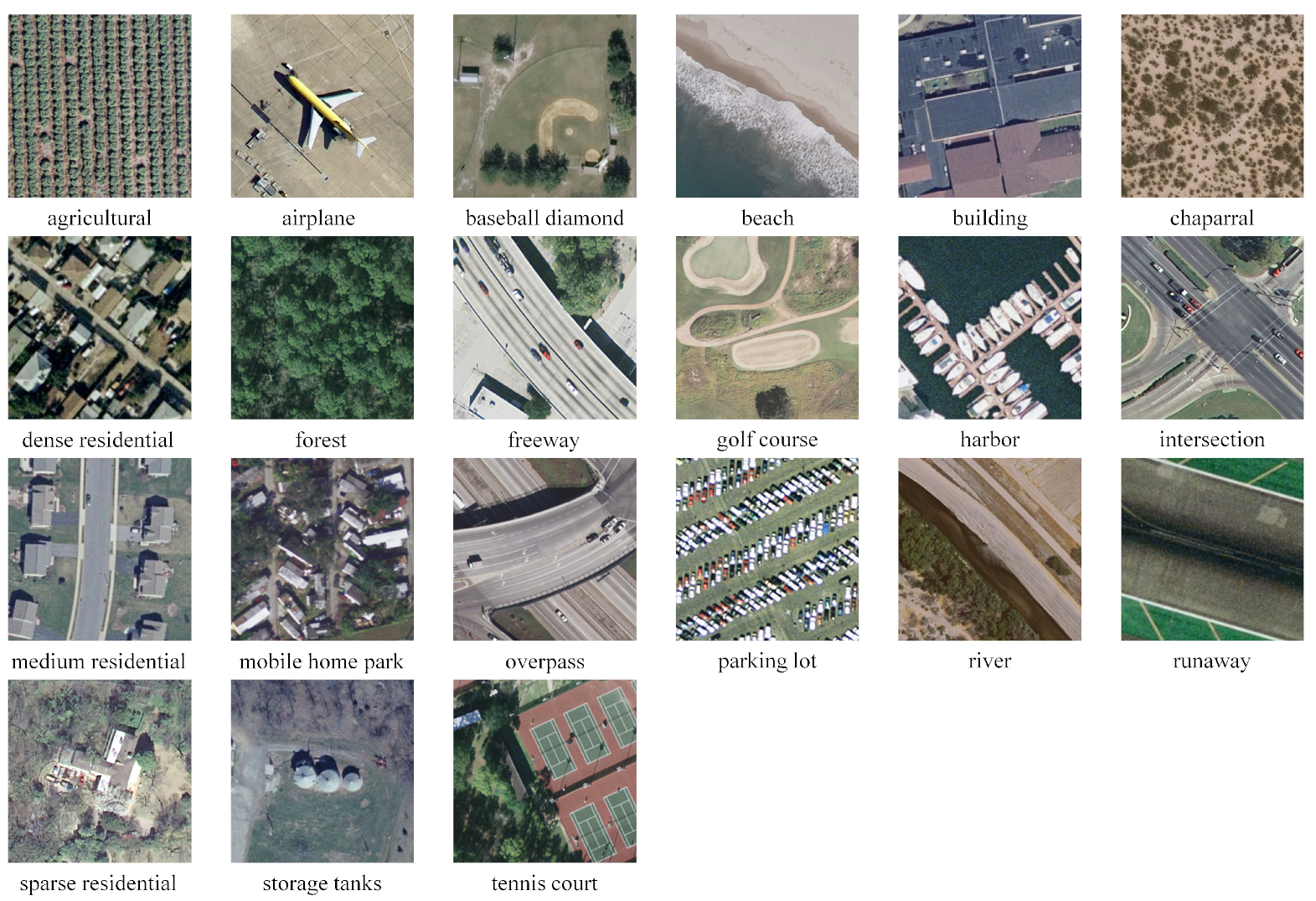
UC Merced [8]: The UC Merced dataset has a total of 2100 aerial images with a fixed size of 256 × 256 and with a pixel resolution of 0.3 m in RGB space. The aerial images are divided into 21 classes, each containing 100 images. When performing the UC Merced evaluation, we randomly chose 80% images from each category for training, and the remaining were used for the test, as introduced in [10,11]. Some samples of the UC Merced dataset are shown in Figure 5.
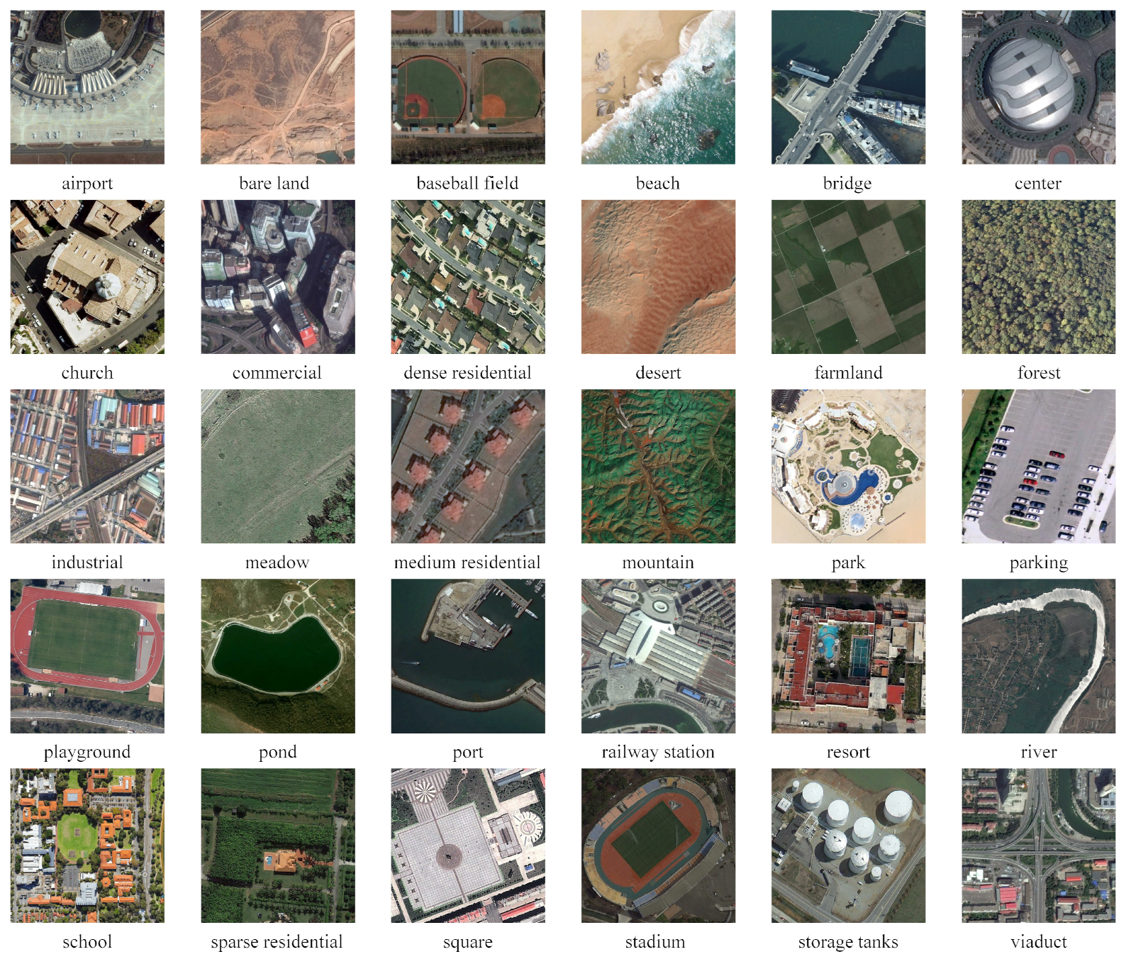
Aerial Image Dataset (AID) [52]: AID dataset includes 10,000 images of 30 classes with spatial resolution from about 8 to 0.5 m. There are 200∼400 images for every category, and each of them is fixed to 600 × 600 pixels. As in [10,11], two dataset partition schemes were applied: 20% and 50% (training set); 80% and 50% (test set). Some samples of AID are shown in Figure 6.
NWPU-RESISC45 [3]: The NWPU-RESISC45 dataset contains 31,500 images covering 45 classes with 700 scene images in each category. These images have 256 × 256 pixels, and the spatial solution varies from about 30 to 0.2 m. We randomly selected 70 (140) images from each category as training images and the other 630 (560) as test images. To date, the NWPU-RESISC45 dataset, as shown in Figure 7, is of the largest in scale, is the most challenging RSISC dataset, and has image variations, high within-class diversity, and high between-class similarity.

3.2. Experimental Setup

In our experiments, we adopted ResNet50 as the backbone network. The proposed MAM replaces each bottleneck of the ResNet50. In the training phase, all images were normalized to 224 × 224 RGB. Data augmentation included random rotation by 45 ; horizontal and vertical flipping. The SGD optimizer was chosen to update network parameters in 100 epochs. We set the batch size, weight decay, and momentum to 32, 0.0005, and 0.9, respectively. The initial learning rate was 0.001 with a 5-epoch warmup and followed the “cosine” policy. The parameter τ in MCAM was empirically set to 16. The weights of cross entropy loss and triplet loss were 1 and 0.5, respectively. The margin of triplet loss was 0.7. In addition, for a fair comparison of our method and some methods using the VGG-16 [58] network as the backbone, we used our method on the VGG-16 network and selected ( F , F ) = { ( C o n v 3 _ 1 , C o n v 3 _ 3 ) , ( C o n v 4 _ 1 , C o n v 4 _ 3 ) , ( C o n v 5 _ 1 , C o n v 5 _ 3 ) } of VGG-16 for building MAM.

3.3. Evaluation Metrics

In the experiment, overall accuracy (OA) and confusion matrix (CM) were used as evaluation indexes for RSISC.
Overall accuracy (OA): This is the ratio of correctly classified samples to all samples. Moreover, we independently repeated 10 runs on three datasets and report the mean and standard deviation of experimental results to show reliable testing results.
Confusion matrix (CM): This is a two-dimensional table to analyze the classification accuracy of each class and the classification confusion between classes. The table has a size of N × N , and N indicates the number of classes. Each row and column represent an image’s true and predicted label, respectively. Diagonals represent the correct prediction of the algorithm, and other positions represent the wrong prediction. Hence, we can intuitively understand the algorithmic performance from the CM this way.

3.4. Compared to State-of-the-Art Methods

This subsection compares the proposed TMGAM with other state-of-art methods on three RSISC datasets. The comparison results on UC Merced, AID, and NWPU-RESISC45 datasets are in Table 1, Table 2 and Table 3.
Table 1 shows the performances of the proposed TMGAM and other methods on the UC Merced dataset. Unlike BoVW [8], other CNN-based methods use VGG-16 or ResNet50 as the basic network and greatly improved the classification accuracy. Classification results of most of them are higher than 99% and are difficult to improve. When using pre-trained ResNet50 or VGG-16 as a backbone, our method achieved good performances of 99.76 % (ResNet50) and 99.29% (VGG-16), respectively.
Table 2 reports the comparison results between our methods and others on AID. The proposed TMGMA with ResNet50 as a backbone outperformed other methods in all cases with classification accuracies of 95.14% and 96.70%, respectively. A similar situation could be found when using VGG-16 as a basic network. Under the training ratio of 50%, the accuracy of our method was slightly lower than the DCNN [11]. Under the training ratio of 50%, our TMGMA achieved the best performance and surpassed DCNN by almost 4%.
In Table 3, we compare our TMGMA with the state-of-art methods of recent years on the NWPU-RESISC45 dataset. The NWPU-RESISC45 dataset is the largest scene classification dataset and can better reflect the classification performances of different methods. Our method with VGG-16 as its backbone is compared with methods using an attention mechanism (SAFF [12], ACNet [47]), metric learning (DCNN [11]), and multi-layer features (MSCP [10], SCCov [33]). Under two different training ratios, our method had improvements of at least 0.5% and 1.8%, respectively. When using ResNet50 as a backbone, the proposed TMGAM achieved higher classification accuracy than most other methods except for the vision transformer [30], which was slightly superior (less than 0.2%) to our method.
In Table 1, Table 2 and Table 3, we compare the proposed TMGMA with the corresponding baseline (i.e., the fine-tuned VGG-16 or the fine-tuned ResNet50) on these three datasets. From baseline to our TMGMA, the experimental results are improved significantly, which indicates the effectiveness of the proposed TMGMA. We also make comparisons between the proposed TMGMA and the CBAM with fine-tuning [44]. Differently from the well-known salient module CBAM, the superiorities of the TMGMA lie in the facts that: (1) our method does not just emphasize semantic regions but selectively focuses on task-related semantic regiones; (2) our method integrates multi-scale information into features; (3) our method mines contextual information from a multi-scale feature map so as to avoid the confusion of features.
In addition, we also compare our method with the recently proposed RSFJR [23] and LGFFE [6]. Compared with RSFJR, an efficient network architecture search framework, the proposed TMGMA aims at mining task-related features. On the NWPU-RESISC45 dataset, the classification accuracies of the RSFJR and our method were 93.68% (60% training samples) and 94.7% (20% training samples). Compared with the LGFFE, using a recurrent neural network (RNN) to capture discriminative features, the proposed TMGMA uses CNN to derive task-related salient features. On the UC Merced and AID datasets, our method can yield the better performance than LGFFE. On the NWPU-RESISC45 dataset, the LGFFE had excellent performances of 97.56% (10% training samples) and 98.79% (20% training samples), which may have been due to the long-term dependencies established by RNN.
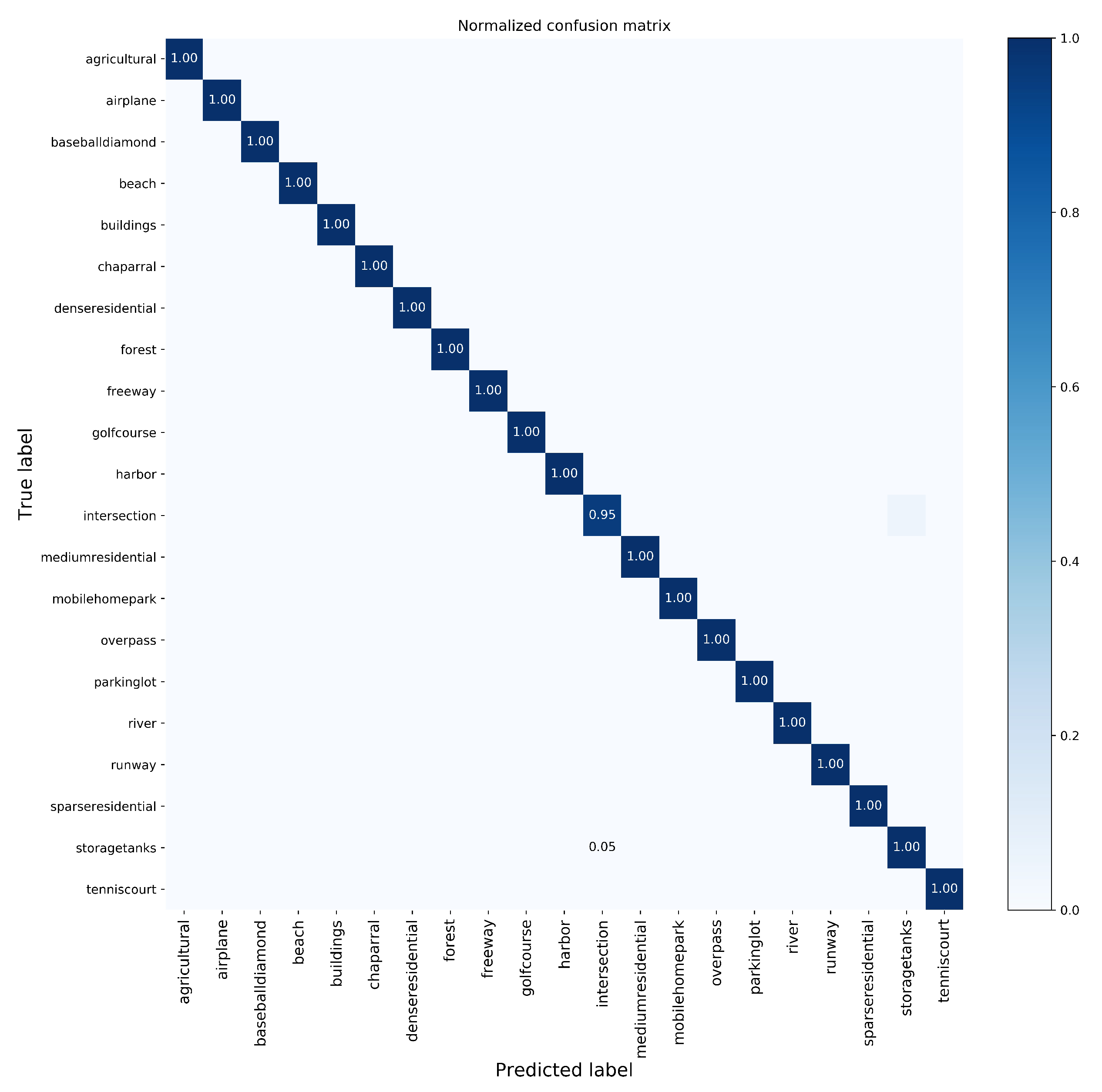
To intuitively analyze the performance of the TMGMA, we drew the confusion matrices (CMs) for the three datasets using the basic network of ResNet50. By testing our algorithm on UC Merced (training ratio = 10%), AID (training ratio = 20%), AID (training ratio = 50%), NWPU (training ratio = 10%), and NWPU (training ratio = 20%), five CMs were obtained and are shown in Figure 8, Figure 9 and Figure 10:
  • The CM of the UC Merced dataset is shown in Figure 8, from which we can see that only the scene class “storagetanks” resulted in classification accuracy of less than 1: 0.95. A “storagetanks” scene was misclassified into “intersection”, since there can be similar objects and appearances. However, our method correctly classified the categories that are easy to be misclassified, e.g., “sparse residential”, “medium residential”, and “dense residential”.
  • The CMs for AID are in Figure 9. With the 20% training ratio, for all 30 categories, only the “school” category has a classification accuracy of less than 90% and is more easily confused with “commercial” and “playground”. For the 50% training ratio, classification accuracies of four categories are less than 90%, but three of them are close to 90%.
  • Figure 10 shows the CMs on the NWPU-RESISC45 dataset when training ratios were 10% and 20%, respectively. With the 10% training ratio, it achieved a classification accuracy of greater than 90% on 37 of 45 scenes and greater than 80% on almost all scenes. With the 20% training ratio, it achieved a classification accuracy of greater than 90% on 40 of 45 scenes and greater than 80% on all scenes. At two different training ratios, we found that the “church” scene and “palace” scene can easily be misclassified into each other because of the similar layout and architectural style.

4. Discussion

4.1. Impact of Multiple Kernels Using Different Combinations

As shown in Table 4, we adjusted the combination using multiple kernels to verify the effectiveness of the proposed TMGMA (based on ResNet50 backbone) on the NWPU-RESISC45 dataset.
In experiments, to avoid increasing the computational cost when capturing multi-scale information, we first performed channel dimension compression in MCAM. Then, convolution operations with different convolution kernels were executed. Let K1, K3, K5, and K7 be the kernels of size 1 × 1 , 3 × 3 , 5 × 5 , and 7 × 7 , respectively. The experiment results are reported in Table 4. From Table 4, we can see that the best classification performance could be obtained using K1 + K3 + K5 + K7. This is because it improves the feature expression for image scene classification.
In our TMGMA, the proposed MAM is guided by multi-scale feature maps, which concatenate the outputs of convolution operations using different convolution kernels. Convolution operations are executed in parallel, and the number of parallel convolutions is proportional to the complexity of the model. With the batch size set to 32 and two NVIDIA GTX 2080Ti GPUs used for acceleration, the time cost of 100 training epochs on the NWPU-RESISC45 is about 150 min. Using K1 + K3 + K5 + K7, the parameter memory of our network increased to 129 MB.

4.2. Effects of Different Components in the Proposed TMGMA

To validate the contributions of different components in TMGMA, we compared seven cases based on the ResNet50 network. The seven cases consistded of (1) ResNet50: one of the backbones for scene classification; (2) ResNet50 + MCAM: the model with multi-scale channel attention; (3) ResNet50 + MSAM: the model with multi-scale spatial attention; (4) ResNet50 + MCAM + MSAM: the model with multi-scale channel and spatial attention; (5) ResNet50 + MAM: the model with MAM-nonidentity and MAM-identity branches; (6) ResNet50 + TM: the model with a triplet metric; (7) ResNet50 + MAM + TM: our whole TMGMA model.
We conducted experiments on the NWPU-RESISC45 dataset and report the results in Table 5. We can see that: (1) all components effectively increased classification accuracy with different improvement degrees; (2) when simultaneously using all components, our method achieved the highest classification performance gain.

4.3. Visualization Using Grad-CAM

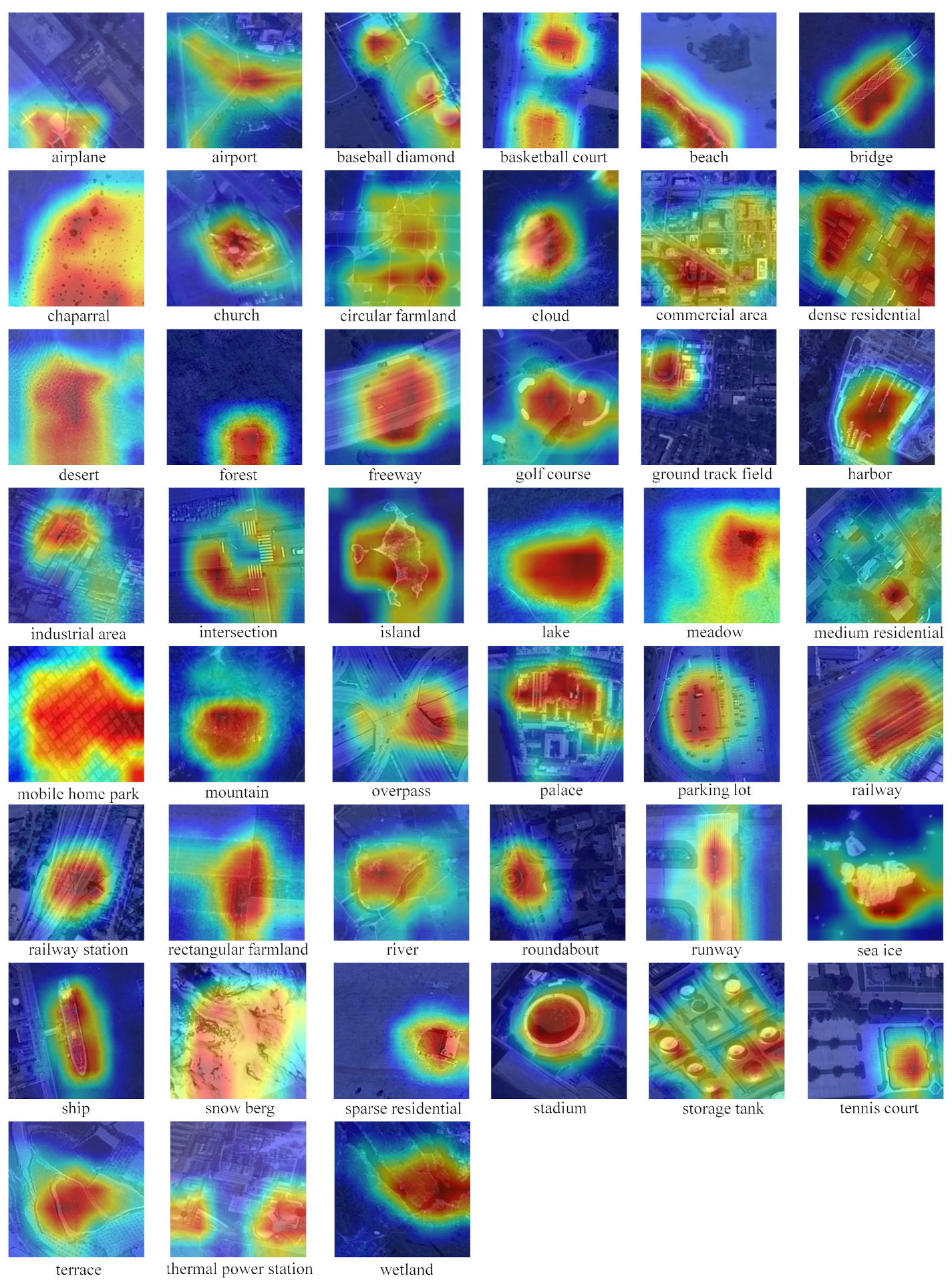
To visually analyze the concerns of our model, a heat map is an effective tool. Here, we chose gradient-weighted class activation mapping (Grad-CAM) [60] to produce visual explanations. As its name implies, Grad-CAM involves flowing the gradients of any target into a convolutional layer to highlight the critical image regions used for predicting the corresponding target.
In our experiments, the Grad-CAM visualized the output of the last convolutional layer using some test samples of the NWPU-RESISC45 dataset. The visualization results are shown in Figure 11. The colors (from blue to red) on a heat map represent different contributions (from small to big) to classification results, the greater the contribution, the redder the color. As shown in Figure 11, it is obvious that the proposed TMGMA (based on the basic network of ResNet50) pays close attention to the task-related semantic region. Furthermore, the red area is mainly concentrated in the central area of the task-related semantic region. The above proves that our method can fully mine contextual information to avoid the feature confusion between the task-related semantic and irrelevant regions.

4.4. Visualization Using t-SNE

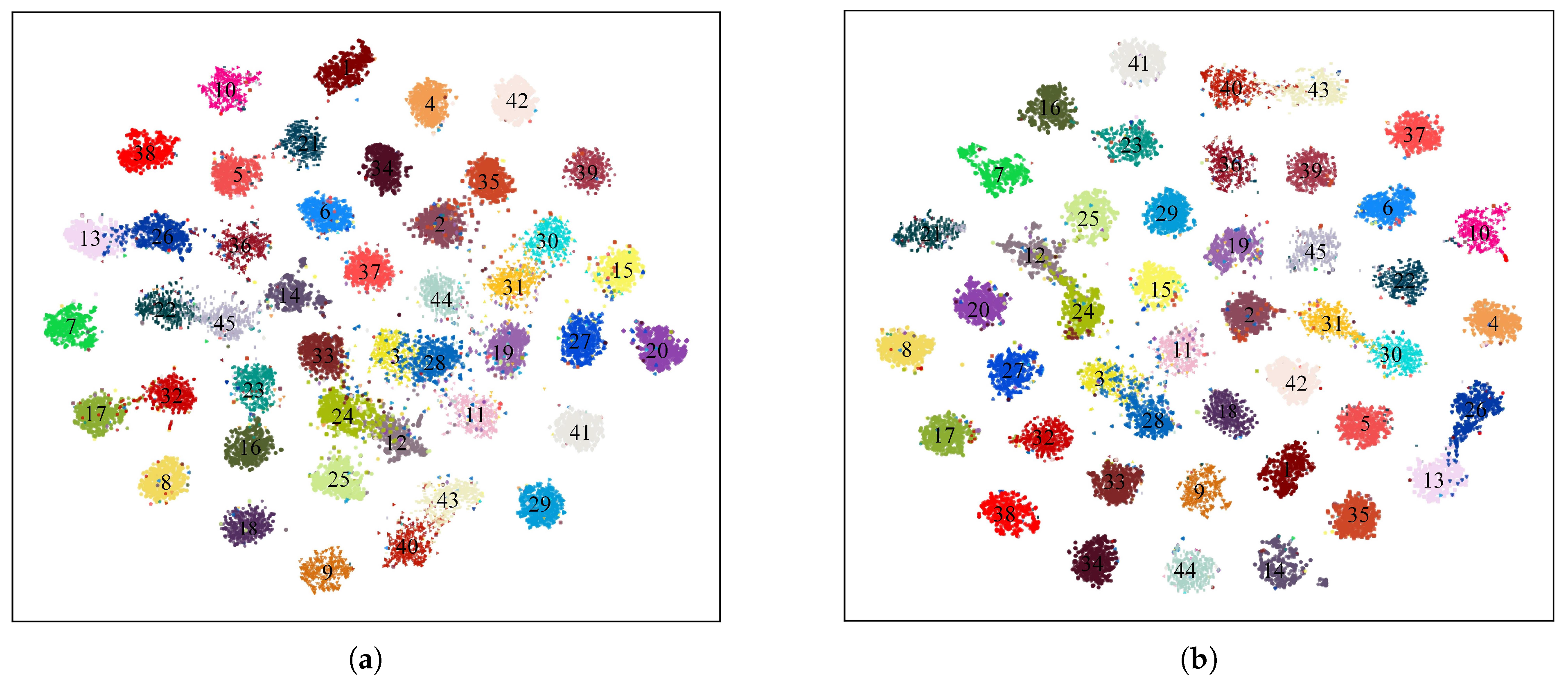
To explore the impact of the proposed TMGMA on feature representation, we applied the t-SNE [61] to visualize high-dimensional features into two-dimensional. In a 2D space, t-SNE can well model the distances of paired data points and distribute a location for each data point.
We performed experiments on the NWPU-RESISC45 dataset. In the experiment, the features of the last FC layer were utilized for visualization. The visualized features are shown in Figure 12 and Figure 13. In Figure 12 and Figure 13, based on two kinds of dataset partitions, i.e., training ratio = 10% and training ratio = 20%, we separately visualize the backbone ResNet50 and the proposed TMGAM (taking the ResNet50 as backbone), respectively. In Figure 12 and Figure 13, we can see clearly that TMGAM can reduce intra-class diversity and inter-class similarity. In feature space, TMGAM makes images in the same category closer and can better distinguish images in different categories so as to improve the classification performance.

5. Conclusions

In this paper, we have presented a novel TMGAM for RSISC. We are committed to learning task-related salient features. Our method involves MAM and TM. MAM performs salient feature extraction and multi-scale and contextual information acquisition. TM is utilized to optimize the MAM to focus on the task-related salient features rather than all salient features. Extensive experiments on three public datasets demonstrated that our approach has good classification results. On the largest scale and most challenging RSISC dataset, i.e., the NWPU-RESISC45, the classification accuracies of the proposed TMGMA (based on ResNet50 backbone) reached 92.44% (training ratio = 10%) and 94.70% (training ratio = 20%).
The proposed TMGMA can emphasize task-related salient features; in other words, it helps to focus on the target area of an image. Hence, our method can be applied to the land-use surveys, natural hazard detection, etc. In the future, we will explore further operators that are potentially applicable to designing effective and efficient RSISC models.

Author Contributions

Conceptualization, H.W.; data curation, H.W. and Y.M.; software, H.W. and L.M.; validation, H.W. and L.M.; formal analysis, X.Z.; writing—original draft preparation, H.W.; writing—review and editing, H.W., K.G., L.M., X.Z., J.W., Z.H. and Y.L.; visualization, H.W., Y.M. and L.M. All authors have read and agreed to the published version of the manuscript.

Funding

This work was supported by the Natural Science Foundation of Beijing Municipality (grant number Z190018) and the National Natural Science Foundation of China (grant numbers 61875013 and 61827814).

Data Availability Statement

The UC Merced Land Use Dataset is this research is openly and freely available at http://weegee.vision.ucmerced.edu/datasets/landuse.html (accessed on 23 April 2022). The Aerial Image Dataset (AID) in this research is openly and freely available at http://www.captain-whu.com/project/AID/ (accessed on 23 April 2022). The NWPU-RESISC45 Dataset is this research is openly and freely available at https://1drv.ms/u/s!AmgKYzARBl5ca3HNaHIlzp_IXjs (OneDrive) or http://pan.baidu.com/s/1mifR6tU (BaiduWangpan) (accessed on 23 April 2022).

Conflicts of Interest

The authors declare no conflict of interest.

References

  1. Yang, K.; Liu, Z.; Lu, Q.; Xia, G. Multi-scale weighted branch network for remote sensing image classification. In Proceedings of the IEEE Conference on Computer Vision and Pattern Recognition (CVPR), Long Beach, CA, USA, 16–20 June 2019; pp. 1–10. [Google Scholar]
  2. Zhang, C.; Sargent, I.; Pan, X.; Li, H.; Atkinson, P.M. Joint deep learning for land cover and land use classification. Remote Sens. Environ. 2019, 221, 173–187. [Google Scholar] [CrossRef] [Green Version]
  3. Cheng, G.; Han, J.; Lu, X. Remote sensing image scene classification: Benchmark and state of the art. Proc. IEEE 2017, 105, 1865–1883. [Google Scholar] [CrossRef] [Green Version]
  4. Cheng, G.; Guo, L.; Zhao, T.; Han, J.; Li, H.; Fang, J. Automatic landslide detection from remote-sensing imagery using a scene classification method based on BoVW and pLSA. Int. J. Remote Sens. 2013, 34, 45–59. [Google Scholar] [CrossRef]
  5. Stumpf, A.; Kerle, N. Object-oriented mapping of landslides using random forests. Remote Sens. Eviron. 2011, 115, 2564–2577. [Google Scholar] [CrossRef]
  6. Lv, Y.; Zhang, X.; Xiong, W.; Cui, Y.; Cai, M. An end-to-end local-global-fusion feature extraction network for remote sensing image scene classification. Remote Sens. 2019, 11, 3006. [Google Scholar] [CrossRef] [Green Version]
  7. Du, Z.; Li, X.; Lu, X. Local structure learning in high resolution remote sensing image retrieval. Neurocomputing 2016, 207, 813–822. [Google Scholar] [CrossRef]
  8. Yang, Y.; Newsam, S. Bag-of-visual-words and spatial extensions for land-use classification. In Proceedings of the 18th ACM SIGSPATIAL International Conference on Advances in Geographic Information Systems, San Jose, CA, USA, 2–5 November 2010; pp. 270–279. [Google Scholar]
  9. Cheng, G.; Han, J.; Guo, L.; Liu, Z.; Bu, S.; Ren, J. Effective and efficient midlevel visual elements-oriented land-use classification using VHR remote sensing images. IEEE Trans. Geosci. Remote Sens. 2015, 53, 4238–4249. [Google Scholar] [CrossRef] [Green Version]
  10. He, N.; Fang, L.; Li, S.; Plaza, A.; Plaza, J. Remote sensing scene classification using multilayer stacked covariance pooling. IEEE Trans. Geosci. Remote Sens. 2018, 56, 6899–6910. [Google Scholar] [CrossRef]
  11. Cheng, G.; Yang, C.; Yao, X.; Guo, L.; Han, J. When deep learning meets metric learning: Remote sensing image scene classification via learning discriminative CNNs. IEEE Trans. Geosci. Remote Sens. 2018, 56, 2811–2821. [Google Scholar] [CrossRef]
  12. Cao, R.; Fang, L.; Lu, T.; He, N. Self-attention-based deep feature fusion for remote sensing scene classification. IEEE Geosci. Remote Sens. Lett. 2020, 18, 43–47. [Google Scholar] [CrossRef]
  13. Lowe, D.G. Distinctive image features from scale-invariant keypoints. Int. J. Comput. Vis. 2004, 60, 91–110. [Google Scholar] [CrossRef]
  14. Ojala, T.; Pietikainen, M.; Maenpaa, T. Multiresolution gray-scale and rotation invariant texture classification with local binary patterns. IEEE Trans. Pattern Anal. Mach. Intell. 2002, 24, 971–987. [Google Scholar] [CrossRef]
  15. Liu, L.; Fieguth, P.; Guo, Y.; Wang, X.; Pietikäinen, M. Local binary features for texture classification: Taxonomy and experimental study. Pattern Recognit. 2017, 62, 135–160. [Google Scholar] [CrossRef] [Green Version]
  16. Dalal, N.; Triggs, B. Histograms of oriented gradients for human detection. In Proceedings of the IEEE Conference on Computer Vision and Pattern Recognition (CVPR), San Diego, CA, USA, 20–26 June 2005; pp. 886–893. [Google Scholar]
  17. Olshausen, B.A.; Field, D.J. Sparse coding with an overcomplete basis set: A strategy employed by V1? Vis. Res. 1997, 37, 3311–3325. [Google Scholar] [CrossRef] [Green Version]
  18. AWold, S.; Esbensen, K.; Geladi, P. Principal component analysis. Chemom. Intell. Lab. Syst. 1987, 2, 37–52. [Google Scholar]
  19. Hinton, G.E.; Salakhutdinov, R.R. Reducing the dimensionality of data with neural networks. Science 2006, 313, 504–507. [Google Scholar] [CrossRef] [PubMed] [Green Version]
  20. Zhu, Q.; Zhong, Y.; Zhao, B.; Xia, G.S.; Zhang, L. Bag-of-visual-words scene classifier with local and global features for high spatial resolution remote sensing imagery. IEEE Geosci. Remote Sens. Lett. 2016, 13, 747–751. [Google Scholar] [CrossRef]
  21. Zhao, B.; Zhong, Y.; Zhang, L. A spectral–structural bag-of-features scene classifier for very high spatial resolution remote sensing imagery. ISPRS J. Photogramm. Remote Sens. 2016, 116, 73–85. [Google Scholar] [CrossRef]
  22. Zou, Q.; Ni, L.; Zhang, T.; Wang, Q. Deep learning based feature selection for remote sensing scene classification. IEEE Geosci. Remote Sens. Lett. 2015, 12, 2321–2325. [Google Scholar] [CrossRef]
  23. Zhang, Z.; Liu, S.; Zhang, Y.; Chen, W. RS-DARTS: A convolutional neural architecture search for remote sensing image scene classification. Remote Sens. 2022, 14, 141. [Google Scholar] [CrossRef]
  24. Längkvist, M.; Kiselev, A.; Alirezaie, M.; Loutfi, A. Classification and segmentation of satellite orthoimagery using convolutional neural networks. Remote Sens. 2016, 8, 329. [Google Scholar] [CrossRef] [Green Version]
  25. Huang, W.; Wang, Q.; Li, X. Feature sparsity in convolutional neural networks for scene classification of remote sensing image. In Proceedings of the IEEE International Geoscience and Remote Sensing Symposium (IGRASS), Yokohama, Japan, 28 July–2 August 2019; pp. 3017–3020. [Google Scholar]
  26. Li, J.; Lin, D.; Wang, Y.; Xu, G.; Zhang, Y.; Ding, C.; Zhou, Y. Deep discriminative representation learning with attention map for scene classification. Remote Sens. 2020, 12, 1366. [Google Scholar] [CrossRef]
  27. Wang, Q.; Liu, S.; Chanussot, J.; Li, X. Scene classification with recurrent attention of VHR remote sensing images. IEEE Trans. Geosci. Remote Sens. 2018, 57, 1155–1167. [Google Scholar] [CrossRef]
  28. Yu, D.; Xu, Q.; Guo, H.; Zhao, C.; Lin, Y.; Li, D. An efficient and lightweight convolutional neural network for remote sensing image scene classification. Sensors 2020, 20, 1999. [Google Scholar] [CrossRef] [PubMed] [Green Version]
  29. Zhao, Z.; Li, J.; Luo, Z.; Li, J.; Chen, C. Remote sensing image scene classification based on an enhanced attention module. IEEE Geosci. Remote Sens. Lett. 2020, 18, 1926–1930. [Google Scholar] [CrossRef]
  30. Bazi, Y.; Bashmal, L.; Rahhal, M.M.A.; Dayil, R.A.; Ajlan, N.A. Vision transformers for remote sensing image classification. Remote Sens. 2021, 13, 516. [Google Scholar] [CrossRef]
  31. Wang, D.; Lan, J. A Deformable Convolutional Neural Network with Spatial-Channel Attention for Remote Sensing Scene Classification. Remote Sens. 2021, 13, 5076. [Google Scholar] [CrossRef]
  32. Liu, Y.; Zhong, Y.; Qin, Q. Scene classification based on multiscale convolutional neural network. IEEE Trans. Geosci. Remote Sens. 2018, 56, 7109–7121. [Google Scholar] [CrossRef] [Green Version]
  33. He, N.; Fang, L.; Li, S.; Plaza, J.; Plaza, A. Skip-connected covariance network for remote sensing scene classification. IEEE Trans. Neural Netw. Learn. Syst. 2020, 31, 1461–1474. [Google Scholar] [CrossRef] [Green Version]
  34. Wang, S.; Guan, Y.; Shao, L. Multi-granularity canonical appearance pooling for remote sensing scene classification. IEEE Trans. Image Process. 2020, 29, 5396–5407. [Google Scholar] [CrossRef] [Green Version]
  35. Zhu, Q.; Zhong, Y.; Zhang, L.; Li, D. Adaptive deep sparse semantic modeling framework for high spatial resolution image scene classification. IEEE Trans. Geosci. Remote Sens. 2018, 56, 6180–6195. [Google Scholar] [CrossRef]
  36. Bi, Q.; Qin, K.; Li, Z.; Zhang, H.; Xu, K.; Xia, G. A multiple-instance densely-connected ConvNet for aerial scene classification. IEEE Trans. Image Process. 2020, 29, 4911–4926. [Google Scholar] [CrossRef] [PubMed]
  37. Fang, J.; Yuan, Y.; Lu, X.; Feng, Y. Robust space–frequency joint representation for remote sensing image scene classification. IEEE Trans. Geosci. Remote Sens. 2019, 57, 7492–7502. [Google Scholar] [CrossRef]
  38. Qi, K.; Yang, C.; Hu, C.; Shen, Y.; Shen, S.; Wu, H. Rotation invariance regularization for remote sensing image scene classification with convolutional neural networks. Remote Sens. 2021, 13, 569. [Google Scholar] [CrossRef]
  39. Bahdanau, D.; Cho, K.; Bengio, Y. Neural machine translation by jointly learning to align and translate. In Proceedings of the International Conference on Learning Representations (ICLR), San Diego, CA, USA, 7–9 May 2015; pp. 1–15. [Google Scholar]
  40. Hu, J.; Shen, L.; Sun, G. Squeeze-and-excitation networks. In Proceedings of the IEEE Conference on Computer Vision and Pattern Recognition (CVPR), Salt Lake City, UT, USA, 18–22 June 2018; pp. 7132–7141. [Google Scholar]
  41. Qin, Z.; Zhang, P.; Wu, F.; Li, X. Fcanet: Frequency channel attention networks. In Proceedings of the IEEE International Conference on Computer Vision (ICCV), Virtual, 11–17 October 2021; pp. 783–792. [Google Scholar]
  42. Wang, Q.; Wu, B.; Zhu, P.; Li, P.; Zuo, W.; Hu, Q. Eca-net: Efficient channel attention for deep convolutional neural networks. In Proceedings of the IEEE Conference on Computer Vision and Pattern Recognition (CVPR), Virtual, 14–19 June 2020. [Google Scholar]
  43. Park, J.; Woo, S.; Lee, J.Y.; Kweon, I.S. Bam: Bottleneck attention module. In Proceedings of the British Machine Vision Conference (BMVC), Newcastle, UK, 3–6 September 2018; pp. 1–14. [Google Scholar]
  44. Woo, S.; Park, J.; Lee, J.Y.; Kweon, I.S. Cbam: Convolutional block attention module. In Proceedings of the European Conference on Computer Vision (ECCV), Munich, Germany, 8–14 September 2018; pp. 3–19. [Google Scholar]
  45. Li, B.; Guo, Y.; Yang, J.; Wang, L.; Wang, Y.; An, W. Gated recurrent multiattention network for VHR remote sensing image classification. IEEE Trans. Geosci. Remote Sens. 2021, 60, 5606113. [Google Scholar] [CrossRef]
  46. Shi, C.; Zhao, X.; Wang, L. A multi-branch feature fusion strategy based on an attention mechanism for remote sensing image scene classification. Remote Sens. 2021, 13, 1950. [Google Scholar] [CrossRef]
  47. Tang, X.; Ma, Q.; Zhang, X.; Liu, F.; Ma, J.; Jiao, L. Attention consistent network for remote sensing scene classification. IEEE J-STARS 2021, 14, 2030–2045. [Google Scholar] [CrossRef]
  48. Song, H.O.; Xiang, Y.; Jegelka, S.; Savarese, S. Deep metric learning via lifted structured feature embedding. In Proceedings of the IEEE Conference on Computer Vision and Pattern Recognition (CVPR), Las Vegas, NV, USA, 26 June–1 July 2016; pp. 4004–4012. [Google Scholar]
  49. Tian, Y.; Chen, C.; Shah, M. Cross-view image matching for geo-localization in urban environments. In Proceedings of the IEEE Conference on Computer Vision and Pattern Recognition (CVPR), Honolulu, HI, USA, 14–19 June 2017; pp. 3608–3616. [Google Scholar]
  50. Cheng, G.; Zhou, P.; Han, J. Duplex metric learning for image set classification. IEEE Trans. Image Process. 2017, 27, 281–292. [Google Scholar] [CrossRef]
  51. Zhang, J.; Lu, C.; Wang, J.; Yue, X.G.; Lim, S.J.; Al-Makhadmeh, Z.; Tolba, A. Training convolutional neural networks with multi-size images and triplet loss for remote sensing scene classification. Sensors 2020, 20, 1188. [Google Scholar] [CrossRef] [Green Version]
  52. Xia, G.; Hu, J.; Hu, F.; Shi, B.; Bai, X.; Zhong, Y.; Zhang, L. AID: A benchmark data set for performance evaluation of aerial scene classification. IEEE Trans. Geosci. Remote Sens. 2017, 55, 3965–3981. [Google Scholar] [CrossRef] [Green Version]
  53. He, K.; Zhang, X.; Ren, S.; Sun, J. Deep residual learning for image recognition. In Proceedings of the IEEE Conference on Computer Vision and Pattern Recognition (CVPR), Las Vegas, NV, USA, 26 June–1 July 2016; pp. 770–778. [Google Scholar]
  54. Ioffe, S.; Szegedy, C. Batch normalization: Accelerating deep network training by reducing internal covariate shift. In Proceedings of the International Conference on Machine Learning (ICML), Lille, France, 6–11 July 2015; pp. 448–456. [Google Scholar]
  55. Nair, V.; Hinton, G.E. Rectified linear units improve restricted boltzmann machines. In Proceedings of the International Conference on Machine Learning (ICML), Haifa, Israel, 21–24 June 2010. [Google Scholar]
  56. Schroff, F.; Kalenichenko, D.; Philbin, J. Facenet: A unified embedding for face recognition and clustering. In Proceedings of the IEEE Conference on Computer Vision and Pattern Recognition (CVPR), Boston, MA, USA, 7–12 June 2015; pp. 815–823. [Google Scholar]
  57. Oveis, A.H.; Giusti, E.; Ghio, S.; Martorella, M. A Survey on the applications of convolutional neural networks for synthetic aperture radar: Recent advances. IEEE Aero. El. Sys. Mag. 2022, 37, 18–42. [Google Scholar] [CrossRef]
  58. Simonyan, K.; Zisserman, A. Very deep convolutional networks for large-scale image recognition. In Proceedings of the International Conference on Learning Representations (ICLR), San Diego, CA, USA, 7–9 May 2015. [Google Scholar]
  59. Sun, H.; Li, S.; Zheng, X.; Lu, X. Remote Sensing Scene Classification by Gated Bidirectional Network. IEEE Trans. Geosci. Remote Sens. 2020, 58, 82–96. [Google Scholar] [CrossRef]
  60. Selvaraju, R.R.; Cogswell, M.; Das, A.; Vedantam, R.; Parikh, D.; Batra, D. Grad-cam: Visual explanations from deep networks via gradient-based localization. In Proceedings of the IEEE International Conference on Computer Vision (ICCV), Venice, Italy, 22–29 October 2017; pp. 618–626. [Google Scholar]
  61. Van der Maaten, L.; Hinton, G. Visualizing data using t-SNE. J. Mach. Learn. Res. 2008, 9, 2579–2605. [Google Scholar]
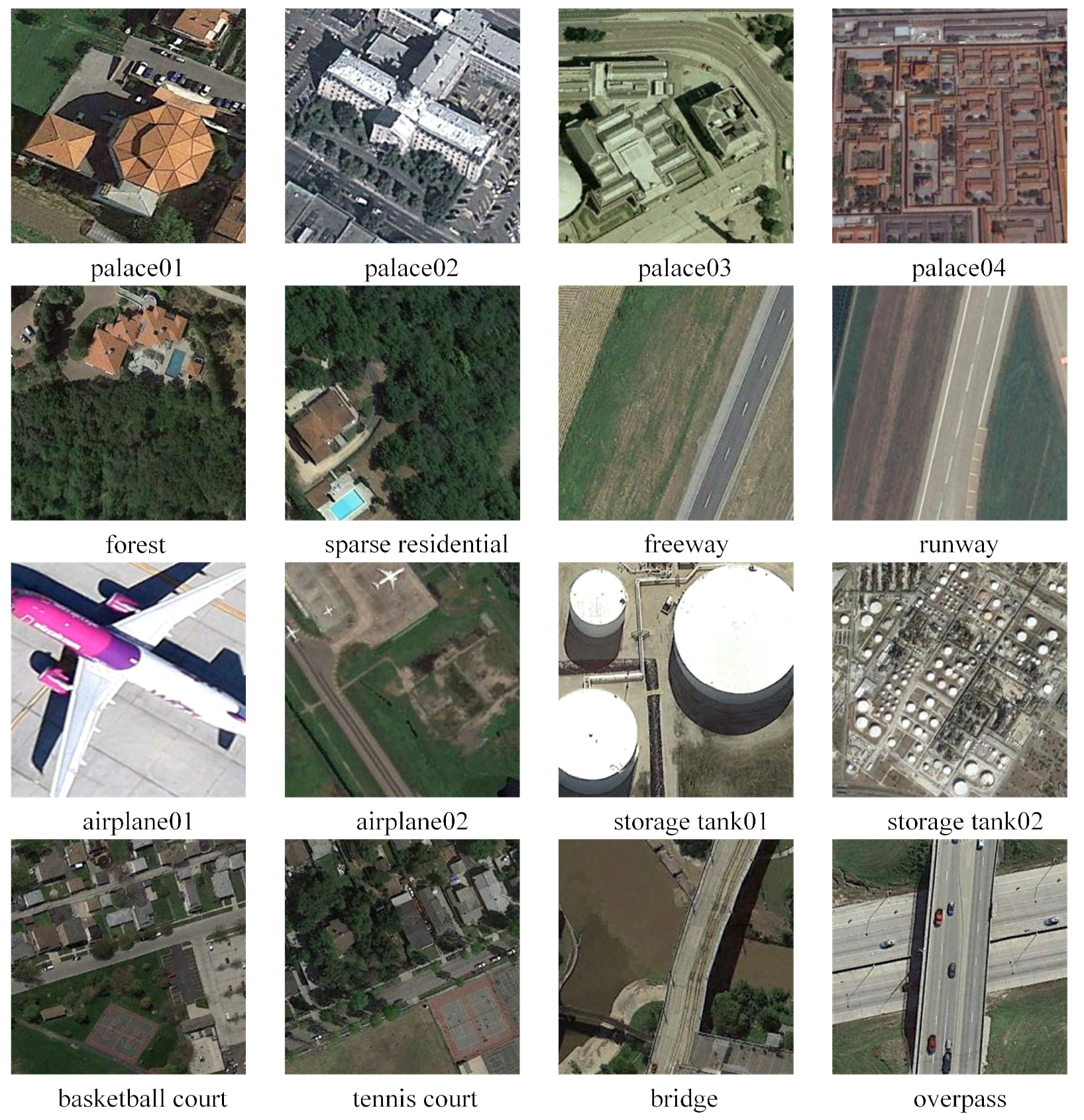
Figure 1. Challenges of RSISC. First row: large diversity within class. Second row: high similarity between classes. Third row: large variance of object/scene scales. Last row: coexistence of multi-class objects. These examples are from the NWPU-RESISC45 dataset [3].
Remotesensing 14 02794 g001
Figure 2. The overall structure of the proposed TMGMA. ⨁ and ⨂ represent element-wise summation and multiplication, respectively.
Remotesensing 14 02794 g002
Figure 3. The structure of the MCAM. We apply appropriate padding to ensure the same output dimension.
Remotesensing 14 02794 g003
Figure 4. The structure of the MSAM. We apply appropriate padding to ensure the same output dimensions.
Remotesensing 14 02794 g004
Figure 5. Some samples of the UC Merced dataset.
Remotesensing 14 02794 g005
Figure 6. Some samples of AID.
Remotesensing 14 02794 g006
Figure 7. Some samples of the NWPU-RESISC45 dataset.
Remotesensing 14 02794 g007
Figure 8. CM on the UC Merced dataset (accuracy = 99.76%).
Remotesensing 14 02794 g008
Figure 9. CMs on AID. (a) Training ratio = 20% (accuracy = 95.14%). (b) Training ratio = 50% (accuracy = 96.70%).
Remotesensing 14 02794 g009
Figure 10. CMs on the NWPU-RESISC45 dataset. (a) Training ratio = 10% (accuracy = 92.44%). (b) Training ratio = 20% (accuracy = 94.70%).
Remotesensing 14 02794 g010
Figure 11. Heat maps generated by Grad-CAM. All samples are from the NWPU-RESISC45 dataset.
Remotesensing 14 02794 g011
Figure 12. Two-dimensional scatterplots of high-dimensional features on the NWPU-RESISC45 dataset (training ratio = 10%). (a) ResNet50 backbone. (b) The proposed TMGAM.
Remotesensing 14 02794 g012
Figure 13. Two-dimensional scatterplots of high-dimensional features on the NWPU-RESISC45 dataset (training ratio = 20%). (a) ResNet50 backbone. (b) The proposed TMGAM.
Remotesensing 14 02794 g013
Table 1. Classification accuracies (%) of the proposed TMGMA and other methods on the UC Merced dataset.
Backbone or FeaturesMethodTraining Ratio (80%)
SIFTBoVW [8]76.81
VGG-16SAFF [12]97.02 ± 0.78
MSCP [10]98.36 ± 0.58
DCNN [11]98.93 ± 0.10
ACNet [47]99.76 ± 0.10
SCCov [33]99.05 ± 0.25
Fine-tuning97.86± 0.12
TMGMA99.29 ± 0.09
ResNet50D-CNN [31]99.62
GBNet [59]98.57 ± 0.48
RIR [38]99.15 ± 0.40
Fine-tuning99.29 ± 0.24
CBAM + Fine-tuning [44]99.42 ± 0.f23
TMGMA99.76 ± 0.04
Table 2. Classification accuracies (%) of the proposed TMGMA and other methods on the AID dataset.
BackboneMethodTraining Ratio (20%)Training Ratio (50%)
VGG-16SAFF [12]90.25 ± 0.2993.83 ± 0.28
MSCP [10]91.52 ± 0.2194.42 ± 0.17
DCNN [11]90.82 ± 0.1696.89 ± 0.10
SCCov [33]93.12 ± 0.2596.10 ± 0.16
ACNet [47]93.33 ± 0.2995.38 ± 0.29
Fine-tuning91.23 ± 0.2294.80 ± 0.14
TMGMA94.65 ± 0.2396.64 ± 0.19
ResNet50D-CNN [31]94.6396.43
GBNet [59]92.20 ± 0.2395.48 ± 0.12
RIR [38]94.95 ± 0.1796.48 ± 0.21
Vision Transformer [30]94.97 ± 0.01-
Fine-tuning94.30 ± 0.1595.24 ± 10
CBAM + Fine-tuning [44]94.66 ± 0.2796.10 ± 0.14
TMGMA95.14 ± 0.2196.70 ± 0.15
Table 3. Classification accuracies (%) of the proposed TMGMA and other methods on the NWPU-RESISC45 dataset.
BackboneMethodTraining Ratio (10%)Training Ratio (20%)
VGG-16SAFF [12]84.38 ± 0.1987.86 ± 0.14
MSCP [10]85.33 ± 0.2188.93 ± 0.14
DCNN [11]89.22 ± 0.5091.89 ± 0.22
SCCov [33]89.30 ± 0.3592.10 ± 0.25
ACNet [47]91.09 ± 0.1392.42 ± 0.16
Fine-tuning86.78 ± 0.3791.35 ± 0.16
TMGMA91.63 ± 0.2194.24 ± 0.17
ResNet50D-CNN [31]89.8894.44
RIR [38]92.05 ± 0.2394.06 ± 0.15
Vision Transformer [30]92.60 ± 0.10-
Fine-tuning90.89 ± 0.1293.36 ± 0.17
CBAM + Fine-tuning [44]91.82 ± 0.1393.94± 0.09
TMGMA92.44 ± 0.1994.70 ± 0.14
Table 4. Results (%) of using different combinations of multiple kernels.
DatasetComponentsAccuracy
NWPU-RESISC45-10%K1 + K392.18
K3 + K592.26
K5 + K791.93
K3 + K5 + K792.27
K1 + K3 + K5 + K792.44
NWPU-RESISC45-20%K1 + K393.97
K3 + K594.31
K5 + K793.61
K3 + K5 + K794.59
K1 + K3 + K5 +K794.70
Table 5. Results (%) for our method with different components on the NWPU-RESISC45 dataset.
DatasetComponentsAccuracy
NWPU-RESISC45-10%ResNet5090.89
ResNet50 + MCAM91.92
ResNet50 + MSAM91.39
ResNet50 + MCAM + MSAM92.14
ResNet50 + MAM92.25
ResNet50 + TM91.39
ResNet50 + MAM + TM92.44
NWPU-RESISC45-20%ResNet5093.36
ResNet50 + MCAM93.94
ResNet50 + MSAM93.63
ResNet50 + MCAM + MSAM94.42
ResNet50 + MAM94.53
ResNet50 + TM93.70
ResNet50 + MAM + TM94.70
Publisher’s Note: MDPI stays neutral with regard to jurisdictional claims in published maps and institutional affiliations.