Abstract
An accurate ego-motion estimation solution is vital for autonomous vehicles. LiDAR is widely adopted in self-driving systems to obtain depth information directly and eliminate the influence of changing illumination in the environment. In LiDAR odometry, the lack of descriptions of feature points as well as the failure of the assumption of uniform motion may cause mismatches or dilution of precision in navigation. In this study, a method to perform LiDAR odometry utilizing a bird’s eye view of LiDAR data combined with a deep learning-based feature point is proposed. Orthographic projection is applied to generate a bird’s eye view image of a 3D point cloud. Thereafter, an R2D2 neural network is employed to extract keypoints and compute their descriptors. Based on those keypoints and descriptors, a two-step matching and pose estimation is designed to keep these feature points tracked over a long distance with a lower mismatch ratio compared to the conventional strategy. In the experiment, the evaluation of the proposed algorithm on the KITTI training dataset demonstrates that the proposed LiDAR odometry can provide more accurate trajectories compared with the handcrafted feature-based SLAM (Simultaneous Localization and Mapping) algorithm. In detail, a comparison of the handcrafted descriptors is demonstrated. The difference between the RANSAC (Random Sample Consensus) algorithm and the two-step pose estimation is also demonstrated experimentally. In addition, the data collected by Velodyne VLP-16 is also evaluated by the proposed solution. The low-drift positioning RMSE (Root Mean Square Error) of 4.70 m from approximately 5 km mileage shown in the result indicates that the proposed algorithm has generalization performance on low-resolution LiDAR.
1. Introduction
Autonomous driving is the trend of intelligent transportation, and high-level self-driving cars require a higher level of positioning accuracy. To obtain robust positioning results, multi-sensor fusion in navigation and localization has been widely researched [1,2,3,4,5,6,7,8]. During localization by multi-sensor fusion, utilizing every single sensor can improve the robustness and accuracy of the entire system. As the primary global positioning method, GNSS (Global Navigation Satellite Systems) can provide high-accuracy position information [9] under ideal conditions. However, it is always vulnerable [10], specifically in urban canyons, where the shadows of buildings and vegetation cause the signal to be interrupted or seriously degraded. LiDAR is an active ranging sensor that can operate under severe conditions and provide accurate depth information directly. By working in an area with a prebuilt map, reliable global positioning results can be obtained by scan matching. However, it is difficult to access a high-quality prebuilt map because of its high cost and limited coverage. Therefore, research on LiDAR odometry is crucial for autonomous driving. Currently, LiDAR odometry includes three main types: geometry-based, deep learning-based, and hybrid methods.
Geometry-based methods consider the geometric information in neighboring areas, utilize curvature to obtain feature points. In [11,12,13,14], researchers extract feature points without descriptors by computing their curvature in a neighbor. A uniform motion model is always adopted to predict the initial pose of the current LiDAR frame. Thereafter, the feature point and closest line or plane are associated with the initial pose. Finally, the relative pose of the LiDAR is estimated by minimizing the distance from point to line and point to plane. Information from adjacent scan lines has not been fully utilized. In [15,16,17], common landmarks extracted from infrastructures in urban areas such as poles and traffic boards were also employed for LiDAR scan matching. These methods are constrained in certain areas and may be ineffective in countries or highways. As there are no descriptors for feature points or landmarks, mismatches can damage the performance of LiDAR odometry. In [18,19], the height map of the 3D LiDAR data was rasterized on the XY plane to generate the image, and direct grayscale matching was utilized to compute the translation and rotation. Xin Zheng [20] combined a spherical image and a bird’s eye view image to perform LiDAR odometry. They adopted a frame-to-model and projected data association to construct the cost function. The authors of [21] proposed a feature-based LiDAR SLAM using the rasterized image. The researchers projected the LiDAR data onto the horizontal plane. Then, they rasterized these 2D points into regular grids and reserved the highest points in each grid to generate BEV (bird’s eye view) image. ORB [22] feature points are extracted on BEV of LiDAR data along with their descriptors. Thereafter, the RANSAC (Random Sample Consensus) algorithm is applied to associate the feature points with their descriptors and geometric consistency. However, these approaches for feature extraction and corresponding feature points can be optimized in a further step for accurate association and longer tracking.
LiDAR odometry methods based on deep learning generally pre-process the point cloud using spherical projection to generate a multi-channel image. The relative pose between the LiDAR frames was estimated by end-to-end inference. LO-Net [23] used a spherical projection image to perform end-to-end LiDAR odometry directly. In the algorithm, multi-channel information was utilized for pose regression and to alleviate the influence of dynamic objects. DeepVCP [24] was trained on a dense point cloud from the accumulated data of Velodyne HDL-64 in 3 s, and 3D feature points were extracted for relative pose estimation. Some researchers have explored unsupervised methods for learning-based LiDAR odometry, such as [25,26], which effectively reduces the data required for training; however, it is difficult to outperform the results using supervised learning. In [25], the researchers trained the network by the result of NICP [27] rather than the ground truth. In [26], the authors proposed unsupervised parameter learning in a Gaussian variational inference setting that is comparable to the ICP [28]. This method is worth further investigation by learning from other fields’ knowledge [29,30,31]. The point cloud pre-processed in the form of spherical projection [23,24,25,26,32,33] makes it challenging to extract local features accurately for low-cost scanning LiDAR, such as Velodyne VLP-16, because of its sparsity. The BEV image is employed in the proposed algorithm to make the algorithm available to process the data of low-resolution LiDAR. Meanwhile, deep learning-based methods have not been investigated for processing the BEV images of LiDAR data in LiDAR odometry, and it is worth exploring.
Another type of method hybridizes the two types of methods above. As the LiDAR odometry can be separated into feature extraction and pose estimation, researchers employ geometry-based and deep learning-based techniques in combination in these two stages. One of the hybrid methods of LiDAR odometry is to use conventional methods to extract feature points and then regress the relative pose of LiDAR frames using a neural network. LodoNet [34] employed SIFT [35] for feature extraction on LiDAR spherical projection images and then rearranged feature point correspondences into n × 6 vectors (each LiDAR point contains three-dimensional coordinates). Finally, convolutional neural networks were trained for feature point culling and regression of relative poses. The other stream of hybrid methods, represented by DMLO [32] and 3D3L [36], extracts and matches the feature points using deep learning on the spherical projection images of LiDAR frames and then performs ICP [28] on the correspondences to obtain the solution by SVD (Singular Value Decomposition) or nonlinear optimization. They keep the common flaw as the end-to-end method by taking the spherical projected image as an input, and it is not necessary to compute the transformation by network modules. Therefore, in this study, the geometry-based pose estimation is adopted.
Three types of methods utilized in LiDAR odometry are summarized above. However, long-distance data association and feature tracking are still obstacles to accuracy improvement. In conventional feature-based LiDAR odometry, feature points are always associated with the closest line or plane, based on the initial guess of the pose [11,12]. In data association with handcrafted descriptors, RANSAC was implemented to determine correspondences. However, a single threshold of distance in the feature space inhibits the algorithms [21,37] by improving the quality of correspondences and length of feature tracking. As a powerful tool for feature extraction, convolutional neural networks have made significant progress in recent years. These networks [38,39,40,41] can extract feature points on images with descriptors and they have outperformed the handcrafted features [22,35,42]. To alleviate these problems, a deep learning-based approach is employed for feature extraction and description. Subsequently, these feature points are culled along with pose estimation using a two-step strategy to perform LiDAR odometry. The main contributions of this study are as follows:
- Accurate LiDAR odometry algorithm using deep learning-based feature point detection and description. Feature points are extracted from the BEV image of the 3D LiDAR data. Accurate and robust keypoint associations than handcrafted feature descriptors can be provided.
- A two-step feature matching and pose estimation strategy is proposed to improve the accuracy of the keypoint association and length of feature tracking. The first step is to ensure the accuracy of the data association, and the second step is to add more reliable feature points for long-range tracking.
- The proposed method is evaluated by processing a commonly used benchmark, the KITTI dataset [43], and it is compared with the SLAM algorithm based on handcrafted feature points. The contributions of deep learning-based feature extraction and two-step pose estimation are verified experimentally. In addition, the generalization of the proposed algorithm is proved by performing field tests using low-resolution LiDAR, Velodyne VLP-16.
2. System Overview
A schematic of the proposed algorithm is shown in Figure 1. The entire pipeline includes pre-processing and LiDAR odometry. Each submodule is executed successively, as shown by the arrows in the figure. The red squares in the flowchart represent the main contributions of this study. In the pre-processing procedure, the LiDAR point cloud is first segmented to retain non-ground points to generate the rasterized image. Subsequently, in the feature extraction stage, R2D2 net is utilized for keypoint extraction and description. Subsequently, the feature points are stored in the map database for further pose estimation and backend optimization.
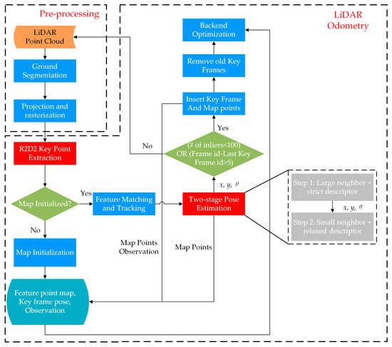
Figure 1.
Workflow of the proposed LiDAR odometry algorithm. Showing the pre-process of LiDAR data and steps involved in mapping, pose estimation, and optimization.
2.1. Pre-Processing
This part corresponds to the pre-processing module shown in Figure 1 in the dotted box. LiDAR receives reflections from the ground during data collection. Because the platform is always in motion, reflections from the ground are not properly utilized in the point-to-point match to estimate the horizontal position. Consequently, LiDAR data are first segmented, keeping non-ground points in the environment for further processing. Because only a few points are reflected from targets at a long distance, in this study, we crop the LiDAR BEV image along the x- and y-axis of the LiDAR (here, we define the x-, y-, and z-axis that point to the right, front, and up direction of the sensor, respectively), leaving a square area of [−37.5 m, 37.5 m]. The retained LiDAR data are then rasterized by orthographic projection, with a resolution of 0.1 m, and the size of the processed image is 750 × 750 pixels. During processing, the highest point z value in each grid is converted to the grayscale of the pixel, and its x and y values are also stored to provide information for subsequent pose optimization. This process is equivalent to a linear transformation of the x- and y-coordinates of the LiDAR frame. The projection transformation is indicated in Equation (1), where and are pixel coordinates, is a coefficient matrix, and and are the origin coordinates of the LiDAR frame. According to the operations described above, and .
For areas without LiDAR reflections, the gray level is uniformly set to 255. After the entire image is rasterized, the grayscale is linearly stretched, and the height value of the original floating-point number is linearly transformed into the range of [0, 255]. In (2), the function limits its output to a certain range of . The is the grayscale of the pixel on the image in the range [0, 255]; is the maximum height value in each grid, and and are the coefficients and bias of linear transformation, respectively.
After converting the LiDAR BEV into an image, it is further processed by Gaussian blur to fill some caverns on the image (isolated grids without LiDAR reflections).
2.2. LiDAR Odometry
This section is part of the dotted box labeled “LiDAR Odometry” in Figure 1. After the pre-processing step mentioned above, R2D2 feature points are extracted for the initialization of the map points and further steps.
2.2.1. Feature Extraction and Matching
This part corresponds to the “R2D2 Keypoint Extraction” and “Feature Matching and Tracking” in Figure 1. Data association in LiDAR odometry is crucial for accuracy as well as the repeatability and reliability of feature points, which are of vital importance in data association. These feature point attributes were considered in the designation of the R2D2 net. It neglects some areas with uniform textures in the optical image, such as the sky, ground, and water surface. Therefore, areas without targets are not the region of interest for the neural network, and no feature points would be extracted in these areas. The pre-processed LiDAR data are input into the R2D2 net as an image, and feature points are extracted along with descriptors and response values. Similar to the response of the handcrafted feature point, the R2D2 feature point uses the product of the repeatability and reliability from the network as the response. The higher the score, the more reliable it is. After keypoint detection, those with the top-k strongest responses are retained. Each feature point is described by a 128-dimensional normalized vector. These descriptors satisfy , where is the ith element of the description vector. In contrast to the ORB descriptor, correlation is used to indicate the similarity between two keypoints rather than the Hamming distance. An example of the keypoints detected by the R2D2 net is shown in Figure 2. The background image is obtained using Equation (1) and filtered by the Gaussian kernel. It can be observed from the distribution of feature points that most of the points are located near points with large gradients in the grayscale domain, such as “corners” and “edges”. In blank areas, only a few feature points will be extracted.
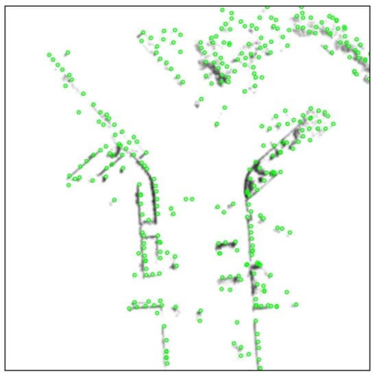
Figure 2.
Keypoints detected by R2D2 net on KITTI dataset. The green circles are keypoints, and the background grayscale image is the BEV of LiDAR data.
In this study, the R2D2 net model is trained on approximately 12,000 optical image pairs for 25 epochs. The settings of filters can be referred to [44]. The sub-sampling grid is set to 16 × 16 for the calculation of repeatability loss. The Adam [45] optimizer was employed to minimize the cost for the R2D2 net. The learning rate was fixed as 0.0001, and the weight decay was set to 0.0005.
2.2.2. Two-Step Pose Estimation
In conventional LiDAR odometry or visual odometry, a uniform motion model is often used to make assumptions. According to the poses of the previous two frames, the initial relative pose of the current frame is obtained by linear interpolation, as in (3).
where and are the relative transformations from frame to frame , including rotation and translation, respectively. Superscript refers to the world frame or map frame, and subscript is the timestamp. is the initial estimation of the relative pose of frame and frame , and is the posterior estimation of the relative pose of frame and map frame . After extracting the feature points of each frame of the image, to avoid searching the entire image, KDTree [46] is employed to store the pixel coordinates of the feature points and search for their correspondences. As shown in Figure 3, the green dotted circle indicates the search radius, and the neighbors are those points within the circle. The red point is the initial guess of the map point in the current LiDAR frame. The blue point is the one most similar to the target (by calculating the correlation coefficient with the target). The other black points are the points projected onto the BEV image.
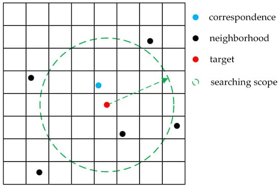
Figure 3.
Radius search on BEV image of LiDAR. The red point is the input target point. The blue point is one of the neighborhoods with the maximum correlation coefficient with the descriptor of the target.
When searching for the first time, because the assumption of a constant speed model is not always suitable for real vehicle motion, there will be greater uncertainty in the pose extrapolation of the current frame. Therefore, a larger search radius is adopted. To avoid mismatches, a strict threshold of descriptor distance is set to confirm the correspondences. Thereafter, each pixel coordinate of the feature point is projected onto the local LiDAR frame using the projection matrix . We then search for the nearest neighbor of this point in the original point cloud. Their coordinates are involved in the cost function for pose optimization by minimizing the distance between the reserved map points and the predicted feature points. An optimized pose can be computed according to (4).
In the second step, because the pose of LiDAR is optimized, we set a smaller neighbor radius to search for correspondences with a relaxed threshold of the distance in the feature space. Here and are the rotation and translation of the current LiDAR frame, respectively, which refer to the map frame . is the reserved map point, and is the ith feature point in the current LiDAR frame corresponding to . In the experiments, the radius of neighbor correspondences is set to 16 pixels, which is the same size as the grid size for repeatability loss of the R2D2 net for the first time, and 3 pixels for the second time.
2.2.3. Map Management
In the map initialization step shown in Figure 1, the position of the first frame is initialized as (0, 0) on the XY plane, and the heading is . All feature points extracted by the network are recovered to the original LiDAR measurement as stated above, and their global coordinates are retained as map points. In the subsequent computation of odometry, for the feature points that are successfully matched, the observation information is associated with the corresponding map points, including the index of the LiDAR frame and global pose of the LiDAR for backend optimization. When inserting a keyframe, the LiDAR point cloud corresponding to all feature points in the frame is transferred to the global frame through the estimated LiDAR pose and marked as a map point for subsequent matching.
2.2.4. Key Frame Selection and Backend Optimization
When the number of tracked inliers is less than 100 points, or there are more than five frames between the last keyframe and the current frame, a keyframe is inserted. In backend optimization, bundle adjustment is used to optimize the pose of the five reserved active keyframes and the associated observations of the map points. The positions of the map points and the poses of the LiDAR keyframes are optimized by minimizing the reprojection error of the associated map points as (5). Here denotes the map point of the j th feature point in the ith frame. and represent the rotation and translation of the LiDAR in frame i referring to the global frame, respectively.
To maintain the number of variables in the backend optimization, we maintain five active keyframes in the backend. The information of the observations and frames out of the sliding window is removed. In general, when a keyframe is to be inserted, it is determined whether the current frame exceeds the distance threshold to the closest keyframe. If it is satisfied, the current keyframe and the corresponding map point observation are not inserted into the map. Otherwise, the earliest active keyframe inserted in the sliding window and the corresponding map points are removed. We apply the ceres [47] library for nonlinear optimization and chose Levenberg-Marquardt as the optimizer.
3. Experiments
The proposed LiDAR odometry algorithm is implemented and evaluated using the KITTI dataset. The data were collected from three types of environments: country, urban, and highway. The types of feature points covered various scenes. The KITTI dataset contains 22 sequences of LiDAR data, where 11 sequences from sequence 00 to sequence 10 are the “training” data. The training data are provided through ground truth translation and rotation.
The data are processed on a laptop with an Intel Core i7-10750H and NVIDIA GeForce GTX 1660 Ti GPU based on Ubuntu 18.04 (Canonical Ltd., London, UK). The processing time of keypoint detection and description is approximately 216 ms/frame, and other parts of the LiDAR odometry are approximately 26 ms/frame on average. The inference process can be at least four times faster on an NVIDIA GeForce GTX 3090 GPU, and odometry can be performed in real time. In addition, data collected by low-resolution LiDAR, VLP-16, are also processed to validate the generalization of the proposed algorithm based on the accuracy of relative motion estimation.
3.1. Evaluation of LiDAR Odometry
In this study, the 2D position on the XY plane and the heading angle are computed using the proposed algorithm. The elevation, roll, and pitch are set to be constant in the odometry estimation. In the first experiment, we used the ATE (Absolute Trajectory Error) to evaluate the performance of LiDAR odometry. According to the method of EVO [48], the predicted trajectory is first aligned with the ground truth trajectory directly, and the z value of the estimated trajectories is set as 0. We then compute the RMSE (Root Mean Square Error) and STD (Standard Deviation) of the position error. The formulas for the RMSE and STD are shown in Equations (8) and (9), respectively. In Equations (6) and (7), is the norm of the translation error of the ith frame, and and is the estimation and ground truth of translation, respectively. represents the number of LiDAR frames in each sequence.
The results of LOAM [11] and “ORB + RANSAC” are obtained from [21]. The results of MULLS [14] are obtained by setting different parameters for different sequences to obtain the best performance of the LiDAR odometry. These parameters are obtained from the configuration files provided by the authors. The z values are then constantly set to 0. However, we set the same parameters for all the sequences. The results are summarized in Table 1. To provide a clear view for readers, the data in the table are rounded to two decimal places without influencing the conclusion, and the trajectories are shown in Figure A1.

Table 1.
Absolute trajectory error of our LiDAR odometry against LOAM and method in [49]. The unit of RMSE and STD is “meters”. The MULLS algorithm is performed by setting different configuration files provided by the author for sequence 01 to obtain the best performances.
The proposed algorithm outperforms the baseline method in most of the sequences according to the RMSE values, even in some sequences with loops such as Seq. 06. As shown in Figure 4, scale errors of the trajectory appear in the results of the ORB feature-based laser SLAM. Loop closure detection and optimization made little contribution to error reduction. Details can be found in the original literature [49].
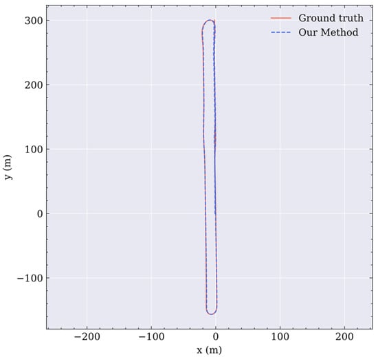
Figure 4.
Trajectory of Seq. 06 in the KITTI dataset by the proposed LiDAR odometry.
This part of the experiment proved the advantage of the combination of deep learning-based feature extraction and two-step pose estimation in LiDAR odometry.
3.2. Performance Comparison between ORB and R2D2 Net
To demonstrate the contribution of deep learning-based feature extraction, we compared the multi-frame tracking performance of the two types of feature points. In the experiment, the frame interval is set to 10 or 20 frames to demonstrate the robustness of the feature extraction against viewing angle changes caused by long-distance movement. We define the average of the matching inliers as an indication of the performance. The more points tracked, the better performance it has.
First, the feature points in the kth frame are transformed into the target frame (k + 10th or k + 20th frame) by the ground truth and projection matrix. Second, the most similar feature point is regarded as a candidate for correspondence. If the distance between their descriptors is below a certain threshold, it is considered an inlier. Similar to [38,41], we set three pixels as the radius when searching for the most similar feature point. Finally, the number of inliers in each pair of frames is counted to compute the average number of inliers for each sequence. The x-axis shows the sequence ID of the data in the KITTI dataset, and the y-axis indicates that the average number of inliers in every sequence satisfies the condition stated above.
Figure 5 shows the average number of inliers for the two types of feature points at 10-frame and 20-frame intervals. The blue bars show the number of inliers detected by the R2D2 net, and the red bars indicate the inliers detected by ORB. The result indicates that R2D2 has a distinct advantage under the condition of a 20-frame interval. This means that more feature points extracted by R2D2 net could be tracked compared to those detected by ORB, and this helps to improve the accuracy by mapping and bundle adjustment in LiDAR odometry.
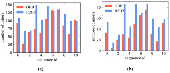
Figure 5.
Tracking inliers comparison of ORB and R2D2 feature extraction. The x-axis is the index of each sequence in the KITTI dataset. (a) The average number of inliers with a 10-frame interval. (b) The average number of inliers with a 20-frame interval.
By analyzing the performance of ORB and R2D2 features further, we provide three reasonable hypotheses as to why the deep learning-based feature extraction method works well on the BEV image of LiDAR data.
- First, there are richer and more complex patterns in optical images than in the BEV LiDAR images. Filters trained by optical images in the network can represent the feature space of the LiDAR BEV images.
- Second, 128-dimensional floating-point descriptors are inferred by the network, leading to a more powerful description of those keypoints than the 256-bit descriptors of the ORB feature.
- Third, the network constructed by a multi-layer convolutional neural network has a larger receptive field to capture global features to make feature points distinguishable.
3.3. Performance Comparison between RANSAC and Two-Step Pose Estimation
To validate the effectiveness of the two-step strategy, a comparison between RANSAC and the two-step pose estimation is performed. In the LiDAR odometry, 100 iterations are set in the RANSAC pose estimation. Except for the feature corresponding process and motion estimation, the other parts of the scheme are the same. The statistical values of LiDAR odometry are listed in Table 2. The results demonstrate that the two-step pose estimation strategy is advantageous.

Table 2.
Absolute trajectory error of two-step data association against RANSAC data association. The unit of RMSE and STD is “meters”.
For an in-depth understanding of the issue, the tracking length of the feature points is analyzed using several keyframes. Referring to the keyframe insertion strategy, the fewer the keyframes inserted, the longer the feature points tracked. The contrasting results are presented in Figure 6. As mentioned above, the strategy of keyframe insertion is set as the interval between the current frame and the last keyframe is larger than five or less than 100 inliers tracked. Using two-step pose estimation, fewer keyframes would be inserted in each sequence, indicating that more keypoints would be tracked longer. The total number of keyframes in LiDAR odometry computed by RANSAC and the two-step pose estimation are shown in different colors.
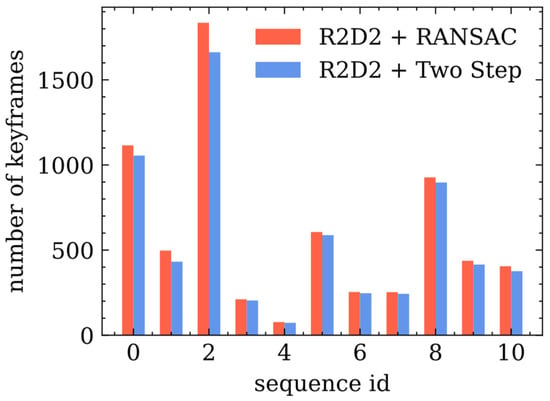
Figure 6.
Number of keyframes inserted by RANSAC and two-step pose estimation.
This part of the experiment verified that the two-step pose estimation strategy improves the performance of feature point tracking.
3.4. Evaluation of Velodyne VLP-16 Dataset
In addition to the KITTI dataset, we tested the generalization of the proposed algorithm on low-resolution LiDAR data. We collected data from the Wuhan Research and Innovation Center, Wuhan City, China, in January 2021. The street view of the park is shown in Figure 7, and the scene is similar to that of the urban environment in the KITTI dataset.
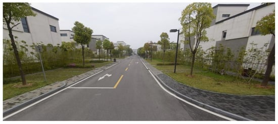
Figure 7.
Wuhan Research and Innovation Center from Baidu Street View.
The data collection setup includes a quasi-navigation-level INS (Inertial Navigation System) LEADOR POS-A15 with a gyroscope bias stability of 0.027°/h and accelerometer bias stability of 15 mGal. The GNSS RTK is also provided in the form of the positioning results. This equipment is mounted on a Haval H6 SUV with a height of approximately 1.7 m. The extended Kalman filter is utilized to obtain the reference trajectory at the centimeter level by fusing the high-level INS and RTK data. The setup of the data collection system is shown in Figure 8.
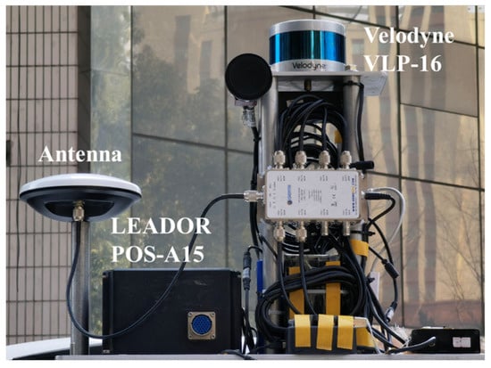
Figure 8.
Setup of the data collecting system.
The data sequence length contains 8399 LiDAR frames and lasted for 14 min. This park is nearly a square, and its span is approximately 400 m in both cross directions. Through EVO trajectory alignment and evaluation, the RMSE is 4.70 m, and the STD is 1.55 m, on the same level as the result from KITTI dataset. There is no significant drift, even without loop closure optimization, which proves the effectiveness and generalization of the proposed algorithm. The results are presented in Figure 9.
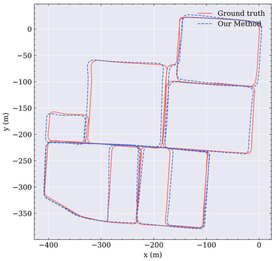
Figure 9.
Trajectory and ground truth of the Wuhan Research and Innovation Center dataset.
4. Conclusions
In this study, we propose an algorithm for 2D LiDAR odometry based on BEV images. Deep learning-based feature extraction and a two-step strategy are combined for pose estimation. The RMSE of the trajectories shows that the proposed method outperforms the corresponding ORB feature-based LiDAR SLAM on the KITTI dataset, even without loop closure in the proposed method. The RMSE of positioning results is reduced compared with that of the baseline method. To prove the effectiveness of the two parts of the algorithm, we compared the performance of feature tracking between R2D2 net and the handcrafted descriptor. The results indicate that the deep learning-based methods can help track more feature points over a long distance. In the experiment comparing RANSAC and the two-step strategy, fewer keyframes are inserted by employing the two-step strategy. An improvement in the feature tracking can also be proved. In addition, we collect low-resolution LiDAR data from Velodyne VLP-16. The results are also presented to validate the generalization of the proposed method. In the result of the evaluation, the RMSE and STD of our dataset are 4.70 m and 1.55 m, respectively, in approximately 5 km long mileage.
Future research will focus on fusing more information from other sensors, such as GNSS, IMU, and wheel encoders, to improve the accuracy and adaptability in a more complex environment. To obtain more practical LiDAR odometry, the network of keypoint detection and description can be optimized by pruning or distillation.
Author Contributions
Collected the data of the experiments, conceived and designed the experiments, performed the experiments, and wrote the paper, T.L.; Gave some advice about the algorithm, Y.W., X.N. and L.C.; Checked the writing of the paper, X.N. and T.Z.; Guided the research direction and offered a platform, J.L. All authors have read and agreed to the published version of the manuscript.
Funding
This research was supported by the National Key Research and Development Program of China (2020YFB0505803) and the National Natural Science Foundation of China (41974024).
Acknowledgments
We want to acknowledge Hailiang Tang for providing a time-synchronizing device and for his help in data collection. We also thank Suhan Huang for his work in the preparation of the experiments.
Conflicts of Interest
The authors declare no conflict of interest.
Appendix A
To provide more details of the results on the KITTI dataset, all trajectories of prediction by the proposed method and the ground truth are shown in Figure A1.
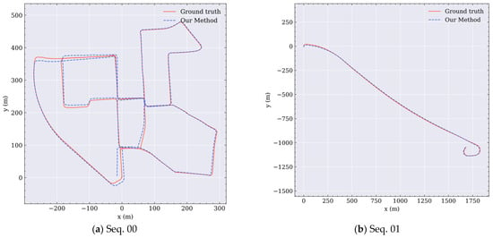
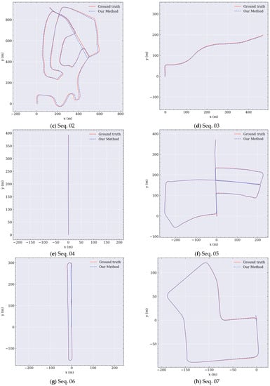
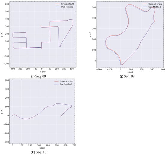
Figure A1.
Prediction trajectories and ground truth of each sequence in the KITTI dataset.
References
- Chang, L.; Niu, X.; Liu, T.; Tang, J.; Qian, C. GNSS/INS/LiDAR-SLAM integrated navigation system based on graph optimization. Remote Sens. 2019, 11, 1009. [Google Scholar] [CrossRef] [Green Version]
- Hengjie, L.; Hong, B.; Cheng, X. Fast Closed-Loop SLAM based on the fusion of IMU and Lidar. J. Phys. Conf. Ser. 2021, 1914, 012019. [Google Scholar] [CrossRef]
- Li, X.; Wang, H.; Li, S.; Feng, S.; Wang, X.; Liao, J. GIL: A tightly coupled GNSS PPP/INS/LiDAR method for precise vehicle navigation. Satell. Navig. 2021, 2, 26. [Google Scholar] [CrossRef]
- Chang, L.; Niu, X.; Liu, T. GNSS/IMU/ODO/LiDAR-SLAM Integrated Navigation System Using IMU/ODO Pre-Integration. Sensors 2020, 20, 4702. [Google Scholar] [CrossRef]
- Li, C.; Sun, H.; Ye, P. Multi-sensor fusion localization algorithm for outdoor mobile robot. J. Phys. Conf. Ser. 2020, 1453, 012042. [Google Scholar] [CrossRef]
- Chiang, K.-W.; Tsai, G.-J.; Li, Y.-H.; Li, Y.; El-Sheimy, N. Navigation engine design for automated driving using INS/GNSS/3D LiDAR-SLAM and integrity assessment. Remote Sens. 2020, 12, 1564. [Google Scholar] [CrossRef]
- Wang, C.; Zhang, G.; Zhang, M. Research on improving LIO-SAM based on Intensity Scan Context. J. Phys. Conf. Ser. 2021, 1827, 012193. [Google Scholar] [CrossRef]
- Wang, W.; Liu, J.; Wang, C.; Luo, B.; Zhang, C. DV-LOAM: Direct visual lidar odometry and mapping. Remote Sens. 2021, 13, 3340. [Google Scholar] [CrossRef]
- Liu, J.; Gao, K.; Guo, W.; Cui, J.; Guo, C. Role, path, and vision of “5G + BDS/GNSS”. Satell. Navig. 2020, 1, 23. [Google Scholar] [CrossRef]
- Du, Y.; Wang, J.; Rizos, C.; El-Mowafy, A. Vulnerabilities and integrity of precise point positioning for intelligent transport systems: Overview and analysis. Satell. Navig. 2021, 2, 3. [Google Scholar] [CrossRef]
- Zhang, J.; Singh, S. LOAM: Lidar Odometry and Mapping in Real-time. Robot. Sci. Syst. 2014, 2, 1–9. [Google Scholar]
- Wang, H.; Wang, C.; Chen, C.-L.; Xie, L. F-LOAM: Fast LiDAR Odometry And Mapping. In Proceedings of the 2021 IEEE/RSJ International Conference on Intelligent Robots and Systems (IROS), Prague, Czech Republic, 27 September–1 October 2021. [Google Scholar]
- Shan, T.; Englot, B. Lego-loam: Lightweight and ground-optimized lidar odometry and mapping on variable terrain. In Proceedings of the 2018 IEEE/RSJ International Conference on Intelligent Robots and Systems (IROS), Madrid, Spain, 1–5 October 2018; pp. 4758–4765. [Google Scholar]
- Pan, Y.; Xiao, P.; He, Y.; Shao, Z.; Li, Z. MULLS: Versatile LiDAR SLAM via multi-metric linear least square. In Proceedings of the 2021 IEEE International Conference on Robotics and Automation (ICRA), Xi’an, China, 30 May–5 June 2021; pp. 11633–11640. [Google Scholar]
- Schaefer, A.; Büscher, D.; Vertens, J.; Luft, L.; Burgard, W. Long-term urban vehicle localization using pole landmarks extracted from 3-D lidar scans. In Proceedings of the 2019 European Conference on Mobile Robots (ECMR), Prague, Czech Republic, 4–6 September 2019; pp. 1–7. [Google Scholar]
- Liu, T.; Chang, L.; Niu, X.; Liu, J. Pole-Like Object Extraction and Pole-Aided GNSS/IMU/LiDAR-SLAM System in Urban Area. Sensors 2020, 20, 7145. [Google Scholar] [CrossRef] [PubMed]
- Steinke, N.; Ritter, C.-N.; Goehring, D.; Rojas, R. Robust LiDAR Feature Localization for Autonomous Vehicles Using Geometric Fingerprinting on Open Datasets. IEEE Robot. Autom. Lett. 2021, 6, 2761–2767. [Google Scholar] [CrossRef]
- Sun, L.; Zhao, J.; He, X.; Ye, C. Dlo: Direct lidar odometry for 2.5 d outdoor environment. In Proceedings of the 2018 IEEE Intelligent Vehicles Symposium (IV), Changshu, China, 26–30 June 2018; pp. 1–5. [Google Scholar]
- Li, J.; Zhao, J.; Kang, Y.; He, X.; Ye, C.; Sun, L. DL-SLAM: Direct 2.5 D LiDAR SLAM for Autonomous Driving. In Proceedings of the 2019 IEEE Intelligent Vehicles Symposium (IV), Paris, France, 9–12 June 2019; pp. 1205–1210. [Google Scholar]
- Zheng, X.; Zhu, J. Efficient LiDAR odometry for autonomous driving. IEEE Robot. Autom. Lett. 2021, 6, 8458–8465. [Google Scholar] [CrossRef]
- Ali, W.; Liu, P.; Ying, R.; Gong, Z. A life-long SLAM approach using adaptable local maps based on rasterized LIDAR images. IEEE Sens. J. 2021, 21, 21740–21749. [Google Scholar] [CrossRef]
- Rublee, E.; Rabaud, V.; Konolige, K.; Bradski, G. ORB: An efficient alternative to SIFT or SURF. In Proceedings of the 2011 International Conference on Computer Vision, Barcelona, Spain, 6–13 November 2011; pp. 2564–2571. [Google Scholar]
- Li, Q.; Chen, S.; Wang, C.; Li, X.; Wen, C.; Cheng, M.; Li, J. Lo-net: Deep real-time lidar odometry. In Proceedings of the IEEE/CVF Conference on Computer Vision and Pattern Recognition, Nashville, TN, USA, 20–25 June 2021; pp. 8473–8482. [Google Scholar]
- Lu, W.; Wan, G.; Zhou, Y.; Fu, X.; Yuan, P.; Song, S. Deepvcp: An end-to-end deep neural network for point cloud registration. In Proceedings of the IEEE/CVF International Conference on Computer Vision, Seoul, Korea, 27 October–2 November 2019; pp. 12–21. [Google Scholar]
- Cho, Y.; Kim, G.; Kim, A. Unsupervised geometry-aware deep lidar odometry. In Proceedings of the 2020 IEEE International Conference on Robotics and Automation (ICRA), Paris, France, 31 May–31 August 2020; pp. 2145–2152. [Google Scholar]
- Yoon, D.J.; Zhang, H.; Gridseth, M.; Thomas, H.; Barfoot, T.D. Unsupervised Learning of Lidar Features for Use ina Probabilistic Trajectory Estimator. IEEE Robot. Autom. Lett. 2021, 6, 2130–2138. [Google Scholar] [CrossRef]
- Serafin, J.; Grisetti, G. NICP: Dense normal based point cloud registration. In Proceedings of the 2015 IEEE/RSJ International Conference on Intelligent Robots and Systems (IROS), Hamburg, Germany, 28 September–2 October 2015; pp. 742–749. [Google Scholar]
- Besl, P.J.; McKay, N.D. Method for registration of 3-D shapes. In Proceedings of the Sensor Fusion IV: Control Paradigms and Data Structures, Boston, MA, USA, 30 April 1992; pp. 586–606. [Google Scholar]
- Zhang, D.; Yao, L.; Chen, K.; Wang, S.; Chang, X.; Liu, Y. Making Sense of Spatio-Temporal Preserving Representations for EEG-Based Human Intention Recognition. IEEE Trans. Cybern. 2020, 50, 3033–3044. [Google Scholar] [CrossRef]
- Luo, M.; Chang, X.; Nie, L.; Yang, Y.; Hauptmann, A.G.; Zheng, Q. An Adaptive Semisupervised Feature Analysis for Video Semantic Recognition. IEEE Trans. Cybern. 2018, 48, 648–660. [Google Scholar] [CrossRef]
- Chen, K.; Yao, L.; Zhang, D.; Wang, X.; Chang, X.; Nie, F. A semisupervised recurrent convolutional attention model for human activity recognition. IEEE Trans. Neural Netw. Learn. Syst. 2019, 31, 1747–1756. [Google Scholar] [CrossRef]
- Li, Z.; Wang, N. Dmlo: Deep matching lidar odometry. In Proceedings of the 2020 IEEE/RSJ International Conference on Intelligent Robots and Systems (IROS), Las Vegas, NV, USA, 24 October–24 January 2021; pp. 6010–6017. [Google Scholar]
- Ambrus, R.; Guizilini, V.; Li, J.; Gaidon, S.P.A. Two stream networks for self-supervised ego-motion estimation. In Proceedings of the Conference on Robot Learning, Osaka, Japan, 30 October–1 November 2019; pp. 1052–1061. [Google Scholar]
- Zheng, C.; Lyu, Y.; Li, M.; Zhang, Z. Lodonet: A deep neural network with 2d keypoint matching for 3d lidar odometry estimation. In Proceedings of the 28th ACM International Conference on Multimedia, Seattle, WA, USA, 12–16 October 2020; pp. 2391–2399. [Google Scholar]
- Lowe, D.G. Object recognition from local scale-invariant features. In Proceedings of the Seventh IEEE International Conference on Computer Vision, Kerkyra, Greece, 20–27 September 1999; pp. 1150–1157. [Google Scholar]
- Streiff, D.; Bernreiter, L.; Tschopp, F.; Fehr, M.; Siegwart, R. 3D3L: Deep Learned 3D Keypoint Detection and Description for LiDARs. arXiv 2021, arXiv:2103.13808. [Google Scholar]
- Ali, W.; Liu, P.; Ying, R.; Gong, Z. 6-DOF Feature based LIDAR SLAM using ORB Features from Rasterized Images of 3D LIDAR Point Cloud. arXiv 2021, arXiv:2103.10678. [Google Scholar]
- Dusmanu, M.; Rocco, I.; Pajdla, T.; Pollefeys, M.; Sivic, J.; Torii, A.; Sattler, T. D2-net: A trainable cnn for joint detection and description of local features. arXiv 2019, arXiv:1905.03561. [Google Scholar]
- Tian, Y.; Fan, B.; Wu, F. L2-net: Deep learning of discriminative patch descriptor in euclidean space. In Proceedings of the IEEE Conference on Computer Vision and Pattern Recognition, Honolulu, HI, USA, 21–26 July 2017; pp. 661–669. [Google Scholar]
- Yi, K.M.; Trulls, E.; Lepetit, V.; Fua, P. Lift: Learned invariant feature transform. In Proceedings of the European Conference on Computer Vision, Amsterdam, The Netherlands, 11–14 October 2016; pp. 467–483. [Google Scholar]
- Revaud, J. R2d2: Reliable and repeatable detectors and descriptors for joint sparse keypoint detection and local feature extraction. In Proceedings of the IEEE Conference on Computer Vision and Pattern Recognition Workshop, Long Beach, CA, USA, 15–20 June 2019. [Google Scholar]
- Bay, H.; Tuytelaars, T.; Van Gool, L. Surf: Speeded up robust features. In Proceedings of the European Conference on Computer Vision, Graz, Austria, 7–13 May 2006; pp. 404–417. [Google Scholar]
- Geiger, A.; Lenz, P.; Urtasun, R. Are we ready for autonomous driving. In Proceedings of the 2012 IEEE Conference on Computer Vision and Pattern Recognition, Providence, RI, USA, 16–21 June 2012; pp. 3354–3361. [Google Scholar]
- Revaud, J.; De Souza, C.; Humenberger, M.; Weinzaepfel, P. R2d2: Reliable and repeatable detector and descriptor. Adv. Neural Inf. Processing Syst. 2019, 32, 12405–12415. [Google Scholar]
- Kingma, D.P.; Ba, J. Adam: A method for stochastic optimization. arXiv 2014, arXiv:1412.6980. [Google Scholar]
- Rusu, R.B.; Cousins, S. 3D is here: Point Cloud Library (PCL). In Proceedings of the 2011 IEEE International Conference on Robotics and Automation (ICRA), Shanghai, China, 9–13 May 2011. [Google Scholar]
- Agarwal, S.; Mierle, K.; Team, T.C.S. Ceres Solver; Google Inc.: Mountain View, CA, USA, 2022. [Google Scholar]
- Grupp, M. evo: Python Package for the Evaluation of Odometry and SLAM. 2017. Available online: https://github.com/MichaelGrupp/evo (accessed on 6 June 2022).
- Ali, W.; Liu, P.; Ying, R.; Gong, Z. A Feature based Laser SLAM using Rasterized Images of 3D Point Cloud. IEEE Sens. J. 2021, 21, 24422–24430. [Google Scholar] [CrossRef]
Publisher’s Note: MDPI stays neutral with regard to jurisdictional claims in published maps and institutional affiliations. |
© 2022 by the authors. Licensee MDPI, Basel, Switzerland. This article is an open access article distributed under the terms and conditions of the Creative Commons Attribution (CC BY) license (https://creativecommons.org/licenses/by/4.0/).