
Remote Sensing of Complex Permittivity and Penetration Depth of Soils Using P-Band SAR Polarimetry

 ,
,  ,
,  ,
,  ,
,  ,
, 
Abstract
:1. Introduction
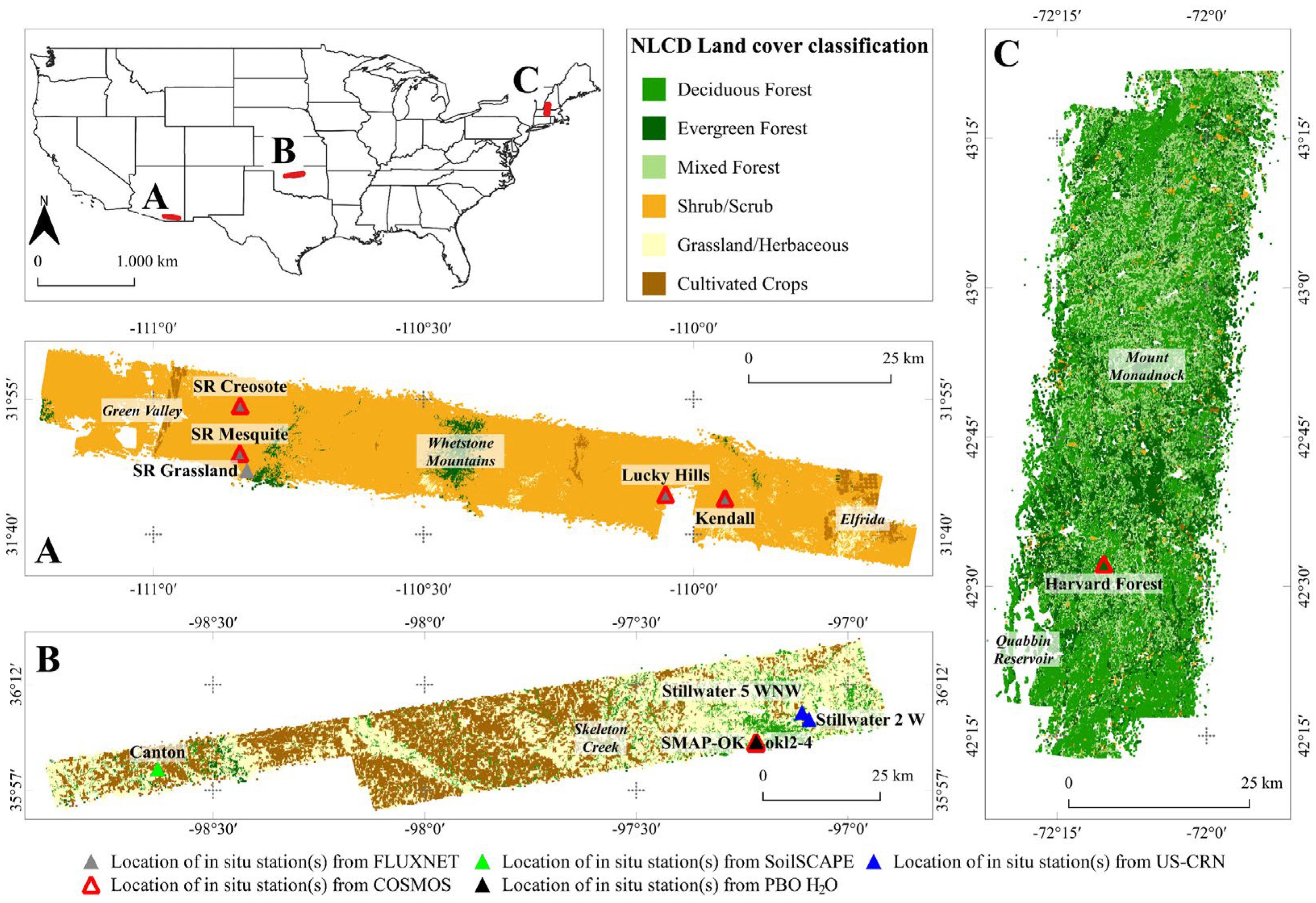
2. Materials
3. Methods
3.1. Soil Scattering Based on Multi-Layer SPM
3.2. Polarimetric Hybrid Decomposition Method
3.3. Complex Permittivity Estimation
4. Results
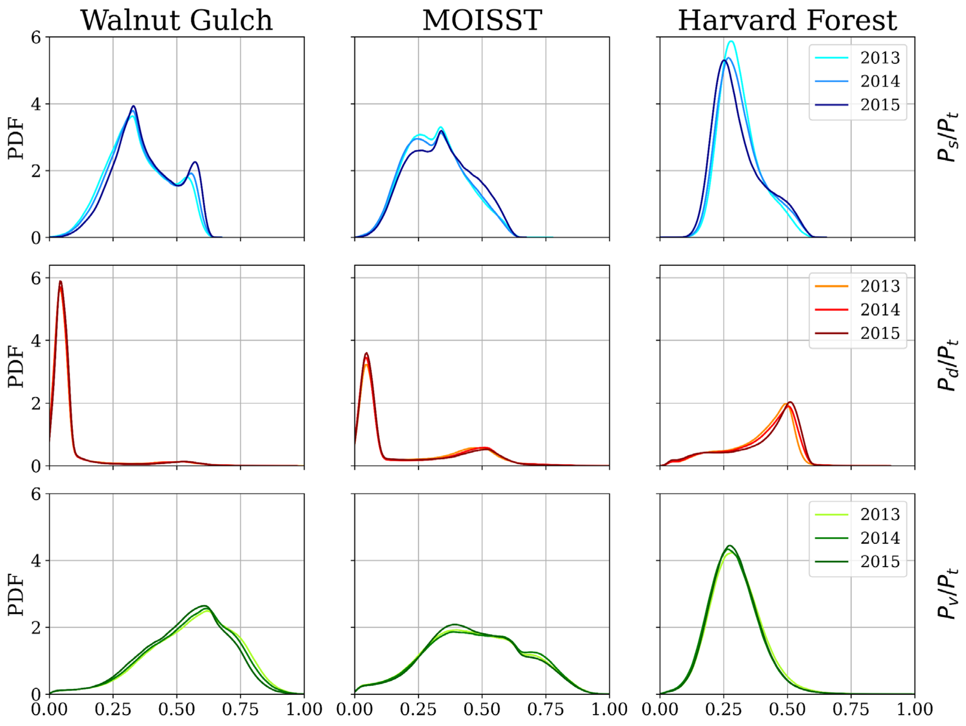
4.1. Decomposition Results
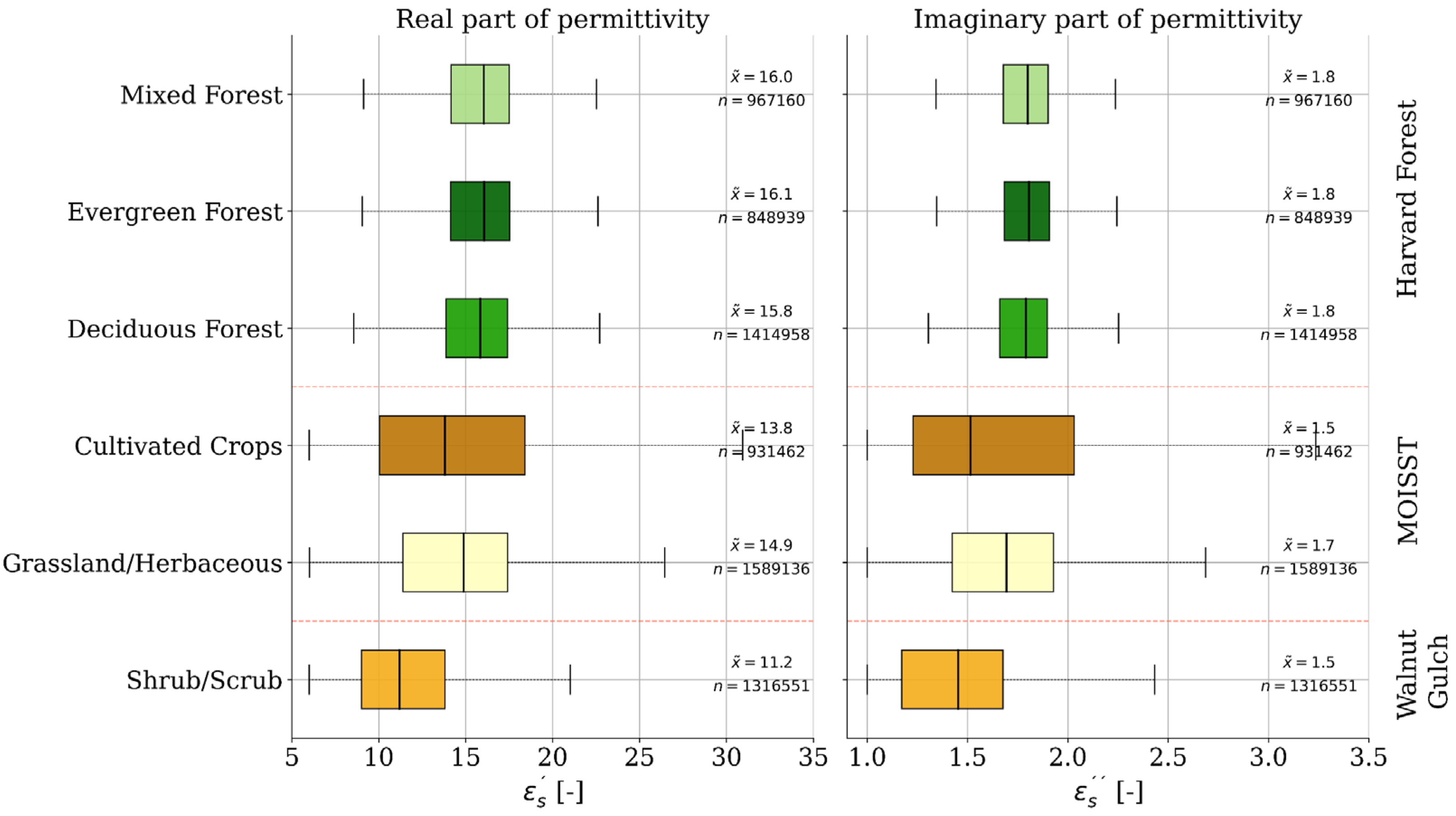
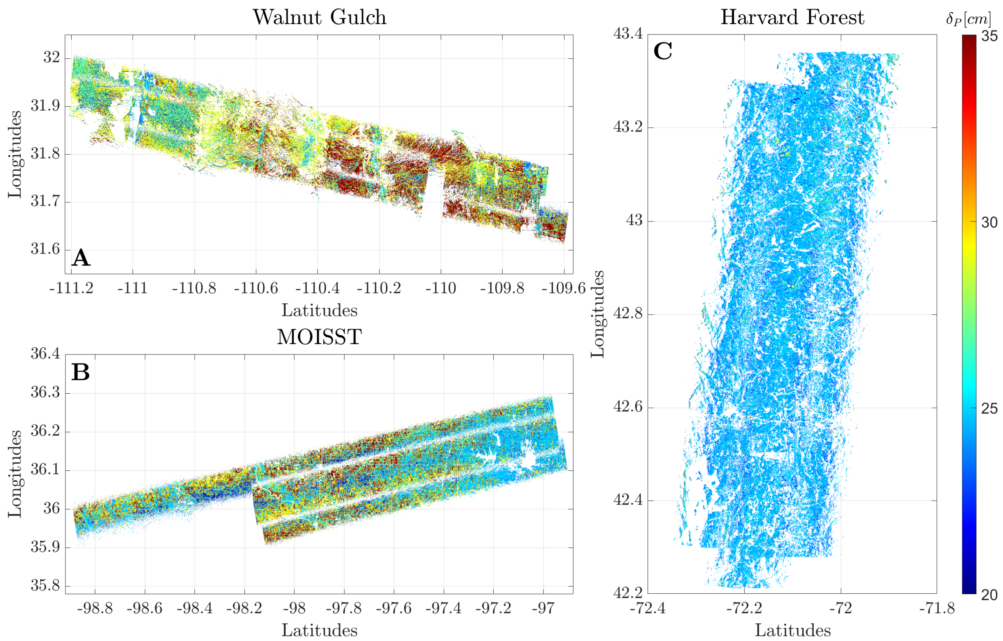
4.2. Results for Complex Soil Permittivity and P-Band Penetration Depth
4.3. Comparison of Permittivity Estimates with In Situ Measurements
5. Discussion
6. Conclusions and Outlook
Author Contributions
Funding
Data Availability Statement
Acknowledgments
Conflicts of Interest
References
- GCOS Status of the Global Observing System for Climate, GCOS Report No. 195. 2015. Available online: https://library.wmo.int/index.php?lvl=notice_display&id=18962 (accessed on 16 March 2021).
- Bojinski, S.; Verstraete, M.; Peterson, T.C.; Richter, C.; Simmons, A.; Zemp, M. The Concept of Essential Climate Variables in Support of Climate Research, Applications, and Policy. Bull. Am. Meteorol. Soc. 2014, 95, 1431–1443. [Google Scholar] [CrossRef]
- Alemohammad, S.H.; Konings, A.G.; Jagdhuber, T.; Moghaddam, M.; Entekhabi, D. Characterization of Vegetation and Soil Scattering Mechanisms across Different Biomes Using P-Band SAR Polarimetry. Remote Sens. Environ. 2018, 209, 107–117. [Google Scholar] [CrossRef] [Green Version]
- Babaeian, E.; Sadeghi, M.; Jones, S.B.; Montzka, C.; Vereecken, H.; Tuller, M. Ground, Proximal, and Satellite Remote Sensing of Soil Moisture. Rev. Geophys. 2019, 57, 530–616. [Google Scholar] [CrossRef] [Green Version]
- Etminan, A.; Tabatabaeenejad, A.; Moghaddam, M. Retrieving Root-Zone Soil Moisture Profile From P-Band Radar via Hybrid Global and Local Optimization. IEEE Trans. Geosci. Remote Sens. 2020, 58, 5400–5408. [Google Scholar] [CrossRef]
- Hoeben, R.; Troch, P.A. Assimilation of Active Microwave Observation Data for Soil Moisture Profile Estimation. Water Resour. Res. 2000, 36, 2805–2819. [Google Scholar] [CrossRef] [Green Version]
- Truong-Loi, M.-L.; Saatchi, S.; Jaruwatanadilok, S. Soil Moisture Estimation Under Tropical Forests Using UHF Radar Polarimetry. IEEE Trans. Geosci. Remote Sens. 2015, 53, 1718–1727. [Google Scholar] [CrossRef]
- Entekhabi, D.; Yueh, S.; De Lannoy, G. SMAP Handbook; NASA: Washington, DC, USA, 2014.
- He, L.; Panciera, R.; Tanase, M.A.; Walker, J.P.; Qin, Q. Soil Moisture Retrieval in Agricultural Fields Using Adaptive Model-Based Polarimetric Decomposition of SAR Data. IEEE Trans. Geosci. Remote Sens. 2016, 54, 4445–4460. [Google Scholar] [CrossRef]
- Kerr, Y.H.; Al-Yaari, A.; Rodriguez-Fernandez, N.; Parrens, M.; Molero, B.; Leroux, D.; Bircher, S.; Mahmoodi, A.; Mialon, A.; Richaume, P.; et al. Overview of SMOS Performance in Terms of Global Soil Moisture Monitoring after Six Years in Operation. Remote Sens. Environ. 2016, 180, 40–63. [Google Scholar] [CrossRef]
- Ulaby, F.T.; Dubois, P.C.; van Zyl, J. Radar Mapping of Surface Soil Moisture. J. Hydrol. 1996, 184, 57–84. [Google Scholar] [CrossRef]
- Wang, H.; Magagi, R.; Goita, K.; Jagdhuber, T.; Hajnsek, I. Evaluation of Simplified Polarimetric Decomposition for Soil Moisture Retrieval over Vegetated Agricultural Fields. Remote Sens. 2016, 8, 142. [Google Scholar] [CrossRef] [Green Version]
- Gelas, C.; Villard, L.; Ferro-Famil, L.; Polidori, L.; Koleck, T.; Daniel, S. Multi-Temporal Speckle Filtering of Polarimetric P-Band SAR Data over Dense Tropical Forests: Study Case in French Guiana for the BIOMASS Mission. Remote Sens. 2021, 13, 142. [Google Scholar] [CrossRef]
- Garrison, J.L.; Shah, R.; Kim, S.; Piepmeier, J.; Vega, M.A.; Spencer, D.A.; Banting, R.; Raymond, J.C.; Nold, B.; Larsen, K.; et al. Analyses Supporting SNoOPI: A P-Band Reflectrometry Demonstration. In Proceedings of the IGARSS 2020—2020 IEEE International Geoscience and Remote Sensing Symposium, Waikoloa, HI, USA, 26 September–2 October 2020; pp. 3349–3352. [Google Scholar]
- NASA. 2019. Available online: https://www.nasa.gov/feature/goddard/2019/snoopi-a-flying-ace-for-soil-moisture-and-snow-measurements (accessed on 16 March 2021).
- Chapin, E.; Chau, A.; Chen, J.; Heavey, B.; Hensley, S.; Lou, Y.; Machuzak, R.; Moghaddam, M. AirMOSS: An Airborne P-Band SAR to Measure Root-Zone Soil Moisture. In Proceedings of the 2012 IEEE Radar Conference, Atlanta, GA, USA, 7–11 May 2012; pp. 693–698. [Google Scholar]
- Alberga, V.; Satalino, G.; Staykova, D.K. Comparison of Polarimetric SAR Observables in Terms of Classification Performance. Int. J. Remote Sens. 2008, 29, 4129–4150. [Google Scholar] [CrossRef]
- Yamaguchi, Y.; Yajima, Y.; Yamada, H. A Four-Component Decomposition of POLSAR Images Based on the Coherency Matrix. IEEE Geosci. Remote Sens. Lett. 2006, 3, 292–296. [Google Scholar] [CrossRef]
- Alemohammad, S.H.; Jagdhuber, T.; Moghaddam, M.; Entekhabi, D. Soil and Vegetation Scattering Contributions in L-Band and P-Band Polarimetric SAR Observations. IEEE Trans. Geosci. Remote Sens. 2019, 57, 8417–8429. [Google Scholar] [CrossRef]
- Cloude, S.R. Uniqueness of Target Decomposition Theorems in Radar Polarimetry. In Direct and Inverse Methods in Radar Polarimetry; Boerner, W.-M., Brand, H., Cram, L.A., Holm, W.A., Stein, D.E., Wiesbeck, W., Keydel, W., Giuli, D., Gjessing, D.T., Molinet, F.A., Eds.; Springer: Dordrecht, The Netherlands, 1992; pp. 267–296. ISBN 978-94-010-9245-6. [Google Scholar]
- Freeman, A.; Durden, S.L. A Three-Component Scattering Model for Polarimetric SAR Data. IEEE Trans. Geosci. Remote Sens. 1998, 36, 963–973. [Google Scholar] [CrossRef] [Green Version]
- van Zyl, J.J.; Arii, M.; Kim, Y. Model-Based Decomposition of Polarimetric SAR Covariance Matrices Constrained for Nonnegative Eigenvalues. IEEE Trans. Geosci. Remote Sens. 2011, 49, 3452–3459. [Google Scholar] [CrossRef]
- Yonezawa, C.; Watanabe, M.; Saito, G. Polarimetric Decomposition Analysis of ALOS PALSAR Observation Data before and after a Landslide Event. Remote Sens. 2012, 4, 2314–2328. [Google Scholar] [CrossRef] [Green Version]
- Jagdhuber, T.; Hajnsek, I.; Papathanassiou, K.P. An Iterative Generalized Hybrid Decomposition for Soil Moisture Retrieval Under Vegetation Cover Using Fully Polarimetric SAR. IEEE J. Sel. Top. Appl. Earth Obs. Remote Sens. 2015, 8, 3911–3922. [Google Scholar] [CrossRef]
- Ballester-Berman, J.D.; Ainsworth, T.L.; Lopez-Sanchez, J.M. On The Physical Quantitative Assessment of Model-Based PolSAR Decompositions. arXiv 2020, arXiv:2001.05872. [Google Scholar]
- Chen, S.-W.; Sato, M.; Wang, X.-S.; Xiao, S.-P. Target Scattering Mechanism in Polarimetric Synthetic Aperture Radar: Interpretation and Application, 1st ed.; Springer: Singapore, 2018; ISBN 978-981-10-7269-7. [Google Scholar]
- Cloude, S. Polarisation: Applications in Remote Sensing, 1st ed.; Oxford University Press: Oxford, UK; New York, NY, USA, 2010; ISBN 978-0-19-956973-1. [Google Scholar]
- Cloude, S.R.; Pottier, E. A Review of Target Decomposition Theorems in Radar Polarimetry. IEEE Trans. Geosci. Remote Sens. 1996, 34, 498–518. [Google Scholar] [CrossRef]
- Hajnsek, I.; Desnos, Y.-L. Polarimetric Synthetic Aperture Radar Principles and Application; Springer: Berlin/Heidelberg, Germany, 2021; ISBN 978-3-030-56504-6. [Google Scholar]
- Van Zyl, J.; Kim, Y. Synthetic Aperture Radar Polarimetry; JPL Space Science and Technology Series; Wiley: Hoboken, NJ, USA, 2011; ISBN 978-1-118-11607-4. [Google Scholar]
- Jagdhuber, T. Soil Parameter Retrieval under Vegetation Cover Using SAR Polarimetry. Ph.D. Thesis, Faculty of Science, University Potsdam, Potsdam, Germany, 2012. Available online: https://publishup.uni-potsdam.de/frontdoor/index/index/docId/5894 (accessed on 18 February 2021).
- Sato, A.; Yamaguchi, Y.; Singh, G.; Park, S.-E. Four-Component Scattering Power Decomposition With Extended Volume Scattering Model. IEEE Geosci. Remote Sens. Lett. 2012, 9, 166–170. [Google Scholar] [CrossRef]
- van Zyl, J.J.; Kim, Y. Requirements for Model-Based Polarimetric Decompositions. In Proceedings of the 7th European Conference on Synthetic Aperture Radar, Friedrichshafen, Germany, 2–5 June 2008. [Google Scholar]
- Kraus, J.D.; Carver, K.R. Electromagnetics, 2nd ed.; McGraw-Hill Electrical and Electronic Engineering Series; McGraw-Hill: New York, NY, USA, 1973; ISBN 978-0-07-035396-1. [Google Scholar]
- Ulaby, F.T.; Long, D.G. Microwave Radar and Radiometric Remote Sensing; The University of Michigan Press: Ann Arbor, MI, USA, 2014; ISBN 978-0-472-11935-6. [Google Scholar]
- Bannawat, L.; Boonpoonga, A.; Akkaraekthalin, P. Permittivity Estimation of a Shallow-Layered Medium Using High-Resolution Ground-Penetrating Radar. Int. J. Remote Sens. 2020, 41, 4626–4643. [Google Scholar] [CrossRef]
- Gururaj, P.; Umesh, P.; Shetty, A. Assessment of Surface Soil Moisture from ALOS PALSAR-2 in Small-Scale Maize Fields Using Polarimetric Decomposition Technique. Acta Geophys. 2021, 69, 579–588. [Google Scholar] [CrossRef]
- Shi, H.; Zhao, L.; Yang, J.; Lopez-Sanchez, J.M.; Zhao, J.; Sun, W.; Shi, L.; Li, P. Soil Moisture Retrieval over Agricultural Fields from L-Band Multi-Incidence and Multitemporal PolSAR Observations Using Polarimetric Decomposition Techniques. Remote Sens. Environ. 2021, 261, 112485. [Google Scholar] [CrossRef]
- Chen, R.H.; Tabatabaeenejad, A.; Moghaddam, M. Retrieval of Permafrost Active Layer Properties Using Time-Series P-Band Radar Observations. IEEE Trans. Geosci. Remote Sens. 2019, 57, 6037–6054. [Google Scholar] [CrossRef]
- Shen, X.; Walker, J.P.; Ye, N.; Wu, X.; Boopathi, N.; Yeo, I.-Y.; Zhang, L.; Zhu, L. Soil Moisture Retrieval Depth of P- and L-Band Radiometry: Predictions and Observations. IEEE Trans. Geosci. Remote Sens. 2020, 59, 6814–6822. [Google Scholar] [CrossRef]
- Ulaby, F.T.; Moore, R.K.; Fung, A.K.; Ulaby, F.T. Microwave Remote Sensing, Active and Passive, Vol. II: Radar Remote Sensing and Surface Scattering and Emission Theory; ARTECH House: Norwood, MA, USA, 1982; Volume 2, ISBN 978-0-201-10760-9. [Google Scholar]
- El Hajj, M.; Baghdadi, N.; Bazzi, H.; Zribi, M. Penetration Analysis of SAR Signals in the C and L Bands for Wheat, Maize, and Grasslands. Remote Sens. 2018, 11, 31. [Google Scholar] [CrossRef] [Green Version]
- Klausing, H.; Holpp, W. Radar Mit Realer Und Synthetischer Apertur: Konzeption und Realisierung; Oldenbourg: München, Germany, 2000; ISBN 978-3-486-23475-6. [Google Scholar]
- Schaber, G.; McCauley, J.; Breed, C.; Olhoeft, G. Shuttle Imaging Radar: Physical Controls on Signal Penetration and Subsurface Scattenng in the Eastern Sahara. IEEE Trans. Geosci. Remote Sens. 1986, GE-24, 603–623. [Google Scholar] [CrossRef]
- Wilheit, T.T. Radiative Transfer in a Plane Stratified Dielectric. IEEE Trans. Geosci. Electron. 1978, 16, 138–143. [Google Scholar] [CrossRef] [Green Version]
- Konings, A.G.; Entekhabi, D.; Moghaddam, M.; Saatchi, S.S. The Effect of Variable Soil Moisture Profiles on P-Band Backscatter. IEEE Trans. Geosci. Remote Sens. 2014, 52, 6315–6325. [Google Scholar] [CrossRef]
- Blumberg, D.G.; Freilikher, V.; Lyalko, I.V.; Vulfson, L.D.; Kotlyar, A.L.; Shevchenko, V.N.; Ryabokonenko, A.D. Soil Moisture (Water-Content) Assessment by an Airborne Scatterometer: The Chernobyl disaster area and the Negev Desert. Remote Sens. Environ. 2000, 71, 309–319. [Google Scholar] [CrossRef]
- Zribi, M.; Sahnoun, M.; Baghdadi, N.; Le Toan, T.; Ben Hamida, A. Analysis of the Relationship between Backscattered P-Band Radar Signals and Soil Roughness. Remote Sens. Environ. 2016, 186, 13–21. [Google Scholar] [CrossRef] [Green Version]
- Ochsner, T.E.; Cosh, M.H.; Cuenca, R.H.; Dorigo, W.A.; Draper, C.S.; Hagimoto, Y.; Kerr, Y.H.; Larson, K.M.; Njoku, E.G.; Small, E.E.; et al. State of the Art in Large-Scale Soil Moisture Monitoring. Soil Sci. Soc. Am. J. 2013, 77, 1888–1919. [Google Scholar] [CrossRef] [Green Version]
- Singh, A.; Meena, G.K.; Kumar, S.; Gaurav, K. Analysis of the Effect of Incidence Angle and Moisture Content on the Penetration Depth of L- and S-Band SAR Signals into the Ground Surface. ISPRS Ann. Photogramm. Remote Sens. Spat. Inf. Sci. 2018, 4, 197–202. [Google Scholar] [CrossRef] [Green Version]
- Tabatabaeenejad, A.; Chen, R.H.; Burgin, M.S.; Duan, X.; Cuenca, R.H.; Cosh, M.H.; Scott, R.L.; Moghaddam, M. Assessment and Validation of AirMOSS P-Band Root-Zone Soil Moisture Products. IEEE Trans. Geosci. Remote Sens. 2020, 58, 6181–6196. [Google Scholar] [CrossRef]
- de Lange, R.; Beck, R.; van de Giesen, N.; Friesen, J.; de Wit, A.; Wagner, W. Scatterometer-Derived Soil Moisture Calibrated for Soil Texture With a One-Dimensional Water-Flow Model. IEEE Trans. Geosci. Remote Sens. 2008, 46, 4041–4049. [Google Scholar] [CrossRef]
- Rao, K.S.; Chandra, G.; Narasimha Rao, P.V. Study on Penetration Depth and Its Dependence on Frequency, Soil Moisture, Texture and Temperature in the Context of Microwave Remote Sensing. J Indian Soc. Remote Sens. 1988, 16, 7–19. [Google Scholar] [CrossRef]
- Moghaddam, M.; Tabatabaeenejad, A.; Chen, R.H.; Saatchi, S.; Jaruwatanadilok, S.; Burgin, M.; Duan, X.; Truong-Loi, M.L. AirMOSS: L2/3 Volumetric Soil Moisture Profiles Derived from Radar, 2012–2015; ORNL DAAC: Oak Ridge, TN, USA, 2016. [CrossRef]
- Peel, M.C.; Finlayson, B.L.; McMahon, T.A. Updated World Map of the Köppen-Geiger Climate Classification. Hydrol. Earth Syst. Sci. 2007, 11, 1633–1644. [Google Scholar] [CrossRef] [Green Version]
- Homer, C.; Dewitz, J.; Yang, L.; Jin, S.; Danielson, P.; Xian, G.; Coulston, J.; Herold, N.; Wickham, J.; Megown, K. Completion of the 2011 National Land Cover Database for the Conterminous United States-Representing a Decade of Land Cover Change Information. Photogramm. Eng. Remote Sens. 2015, 81, 345–354. [Google Scholar]
- Pastorello, G.; Trotta, C.; Canfora, E.; Chu, H.; Christianson, D.; Cheah, Y.W.; Poindexter, C.; Chen, J.; Elbashandy, A.; Humphrey, M.; et al. The FLUXNET2015 Dataset and the ONEFlux Processing Pipeline for Eddy Covariance Data. Sci. Data 2020, 7, 225. [Google Scholar] [CrossRef]
- Montzka, C.; Bogena, H.; Zreda, M.; Monerris, A.; Morrison, R.; Muddu, S.; Vereecken, H. Validation of Spaceborne and Modelled Surface Soil Moisture Products with Cosmic-Ray Neutron Probes. Remote Sens. 2017, 9, 103. [Google Scholar] [CrossRef] [Green Version]
- Zreda, M.; Shuttleworth, W.J.; Zeng, X.; Zweck, C.; Desilets, D.; Franz, T.; Rosolem, R. COSMOS: The COsmic-Ray Soil Moisture Observing System. Hydrol. Earth Syst. Sci. 2012, 16, 4079–4099. [Google Scholar] [CrossRef] [Green Version]
- Moghaddam, M.; Silva, A.; Clewley, D.; Akbar, R.; Hussaini, S.A.; Whitcomb, J.; Devarakonda, R.; Shrestha, R.; Cook, R.B.; Prakash, G.; et al. Soil Moisture Profiles and Temperature Data from SoilSCAPE Sites, USA; ORNL DAAC: Oak Ridge, TN, USA, 2016. [CrossRef]
- Bell, J.E.; Palecki, M.A.; Baker, C.B.; Collins, W.G.; Lawrimore, J.H.; Leeper, R.D.; Hall, M.E.; Kochendorfer, J.; Meyers, T.P.; Wilson, T.; et al. U.S. Climate Reference Network Soil Moisture and Temperature Observations. J. Hydrometeorol. 2013, 14, 977–988. [Google Scholar] [CrossRef]
- Larson, K.M.; Small, E.E.; Gutmann, E.D.; Bilich, A.L.; Braun, J.J.; Zavorotny, V.U. Use of GPS Receivers as a Soil Moisture Network for Water Cycle Studies. Geophys. Res. Lett. 2008, 35, L24405. [Google Scholar] [CrossRef] [Green Version]
- Tabatabaeenejad, A.; Moghaddam, M. Bistatic Scattering from Three-Dimensional Layered Rough Surfaces. IEEE Trans. Geosci. Remote Sens. 2006, 44, 2102–2114. [Google Scholar] [CrossRef]
- Tsang, L.; Kong, J.A.; Shin, R.T. Theory of Microwave Remote Sensing; Wiley Series in Remote Sensing; Wiley: New York, NY, USA, 1985; ISBN 978-0-471-88860-4. [Google Scholar]
- Nicolaides, A. Pure Mathematics: Complex Numbers; P.A.S.S: London, UK, 2008; Volume 3, ISBN 978-1-872684-92-5. [Google Scholar]
- Rizzoli, P.; Martone, M.; Gonzalez, C.; Wecklich, C.; Borla Tridon, D.; Bräutigam, B.; Bachmann, M.; Schulze, D.; Fritz, T.; Huber, M.; et al. Generation and Performance Assessment of the Global TanDEM-X Digital Elevation Model. ISPRS J. Photogramm. Remote Sens. 2017, 132, 119–139. [Google Scholar] [CrossRef] [Green Version]
- GDAL/OGR contributors GDAL/OGR Geospatial Data Abstraction Software Library. Open Source Geospatial Foundation. 2021. Available online: https://Gdal.Org (accessed on 16 March 2021).
- QGIS Development Team QGIS Geographic Information System. Open Source Geospatial Foundation Project. 2021. Available online: http://Qgis.Osgeo.Org (accessed on 16 March 2021).
- Szigarski, C.; Jagdhuber, T.; Baur, M.; Thiel, C.; Parrens, M.; Wigneron, J.-P.; Piles, M.; Entekhabi, D. Analysis of the Radar Vegetation Index and Potential Improvements. Remote Sens. 2018, 10, 1776. [Google Scholar] [CrossRef] [Green Version]
- Kelleners, T.J.; Robinson, D.A.; Shouse, P.J.; Ayars, J.E.; Skaggs, T.H. Frequency Dependence of the Complex Permittivity and Its Impact on Dielectric Sensor Calibration in Soils. Soil Sci. Soc. Am. J. 2005, 69, 67–76. [Google Scholar] [CrossRef]
- Topp, G.C.; Davis, J.L.; Annan, A.P. Electromagnetic Determination of Soil Water Content: Measurements in Coaxial Transmission Lines. Water Resour. Res. 1980, 16, 574–582. [Google Scholar] [CrossRef] [Green Version]
- Dobson, M.; Ulaby, F.; Hallikainen, M.; El-rayes, M. Microwave Dielectric Behavior of Wet Soil-Part II: Dielectric Mixing Models. IEEE Trans. Geosci. Remote Sens. 1985, GE-23, 35–46. [Google Scholar] [CrossRef]
- Mironov, V.L.; Kosolapova, L.G.; Fomin, S.V. Physically and Mineralogically Based Spectroscopic Dielectric Model for Moist Soils. IEEE Trans. Geosci. Remote Sens. 2009, 47, 2059–2070. [Google Scholar] [CrossRef]
- Park, C.-H.; Behrendt, A.; LeDrew, E.; Wulfmeyer, V. New Approach for Calculating the Effective Dielectric Constant of the Moist Soil for Microwaves. Remote Sens. 2017, 9, 732. [Google Scholar] [CrossRef] [Green Version]
- von Hippel, A.R. Dielectrics and Waves; Wiley: New York, NY, USA, 1954. [Google Scholar]
- Mironov, V.L.; Dobson, M.C.; Kaupp, V.H.; Komarov, S.A.; Kleshchenko, V.N. Generalized Refractive Mixing Dielectric Model for Moist Soils. In Proceedings of the IEEE International Geoscience and Remote Sensing Symposium, Toronto, ON, Canada, 24–28 June 2002; Volume 6, pp. 3556–3558. [Google Scholar]
- Moghaddam, M.; Saatchi, S. Analysis of Scattering Mechanisms in SAR Imagery over Boreal Forest: Results from BOREAS ’93. IEEE Trans. Geosci. Remote Sens. 1995, 33, 1290–1296. [Google Scholar] [CrossRef] [Green Version]
- Lucas, R.M.; Moghaddam, M.; Cronin, N. Microwave Scattering from Mixed-Species Forests, Queensland, Australia. IEEE Trans. Geosci. Remote Sens. 2004, 42, 2142–2159. [Google Scholar] [CrossRef]
- Das, N.N.; Mohanty, B.P.; Cosh, M.H.; Jackson, T.J. Modeling and Assimilation of Root Zone Soil Moisture Using Remote Sensing Observations in Walnut Gulch Watershed during SMEX04. Remote Sens. Environ. 2008, 112, 415–429. [Google Scholar] [CrossRef]
- Sivandran, G.; Bras, R.L. Dynamic Root Distributions in Ecohydrological Modeling: A Case Study at Walnut Gulch Experimental Watershed. Water Resour. Res. 2013, 49, 3292–3305. [Google Scholar] [CrossRef]
- Tabatabaeenejad, A.; Burgin, M.; Duan, X.; Moghaddam, M. P-Band Radar Retrieval of Subsurface Soil Moisture Profile as a Second-Order Polynomial: First AirMOSS Results. IEEE Trans. Geosci. Remote Sens. 2015, 53, 645–658. [Google Scholar] [CrossRef]
- Jagdhuber, T. An Approach to Extended Fresnel Scattering for Modeling of Depolarizing Soil-Trunk Double-Bounce Scattering. Remote Sens. 2016, 8, 818. [Google Scholar] [CrossRef] [Green Version]


| NLCD Land Cover Class | AirMOSS Monitoring Site | ||
|---|---|---|---|
| Walnut Gulch | MOISST | Harvard Forest | |
| Grassland/herbaceous | 2.2 | 51.5 | 0.3 |
| Shrub/scrub | 92.5 | 0 | 1.8 |
| Cultivated crops | 2.2 | 38.3 | 0.3 |
| Deciduous forest | <0.1 | 8.3 | 49 |
| Evergreen forest | 3 | 1.7 | 25.1 |
| Mixed forest | <0.1 | 0.3 | 30.4 |
| Parameter | Value |
|---|---|
| Frequency, [MHz] | 430 |
| Number of layers, [–] | 2 |
| Incidence angle in range, , and azimuth, [°] | from AirMOSS; |
| Scattering angle in range , and azimuth, [°] | ; |
| z-coordinates of the respective boundary layer, [cm] | |
| Surface roughness parameters of each layer [cm] (vertical RMS height s, horizontal correlation length l) | , , , and are dependent on roughness indicator derived from TanDEM-X (Table 3, right column) |
| Autocorrelation function, [–] | Exponential |
| Complex permittivity of each layer [–] |
| Roughness Indicator from TanDEM-X [m] | Input Roughness Parameters [cm] |
|---|---|
| < 5 | ; ; ; |
| 5 ≤ < 10 | ; ; ; |
| 10 ≤ < 15 | ; ; ; |
| ≥ 15 | ; ; ; |
Publisher’s Note: MDPI stays neutral with regard to jurisdictional claims in published maps and institutional affiliations. |
© 2022 by the authors. Licensee MDPI, Basel, Switzerland. This article is an open access article distributed under the terms and conditions of the Creative Commons Attribution (CC BY) license (https://creativecommons.org/licenses/by/4.0/).
Share and Cite
Fluhrer, A.; Jagdhuber, T.; Tabatabaeenejad, A.; Alemohammad, H.; Montzka, C.; Friedl, P.; Forootan, E.; Kunstmann, H. Remote Sensing of Complex Permittivity and Penetration Depth of Soils Using P-Band SAR Polarimetry. Remote Sens. 2022, 14, 2755. https://doi.org/10.3390/rs14122755
Fluhrer A, Jagdhuber T, Tabatabaeenejad A, Alemohammad H, Montzka C, Friedl P, Forootan E, Kunstmann H. Remote Sensing of Complex Permittivity and Penetration Depth of Soils Using P-Band SAR Polarimetry. Remote Sensing. 2022; 14(12):2755. https://doi.org/10.3390/rs14122755
Chicago/Turabian StyleFluhrer, Anke, Thomas Jagdhuber, Alireza Tabatabaeenejad, Hamed Alemohammad, Carsten Montzka, Peter Friedl, Ehsan Forootan, and Harald Kunstmann. 2022. "Remote Sensing of Complex Permittivity and Penetration Depth of Soils Using P-Band SAR Polarimetry" Remote Sensing 14, no. 12: 2755. https://doi.org/10.3390/rs14122755
APA StyleFluhrer, A., Jagdhuber, T., Tabatabaeenejad, A., Alemohammad, H., Montzka, C., Friedl, P., Forootan, E., & Kunstmann, H. (2022). Remote Sensing of Complex Permittivity and Penetration Depth of Soils Using P-Band SAR Polarimetry. Remote Sensing, 14(12), 2755. https://doi.org/10.3390/rs14122755