Article

Triple Collocation Analysis of Satellite Precipitation Estimates over Australia

1
School of Earth, Atmosphere and Environment, Monash University, Clayton 3800, Australia
2
Long-Range Forecasts, Bureau of Meteorology, Docklands 3008, Australia
3
SPACE Research Centre, School of Science, Royal Melbourne Institute of Technology (RMIT) University, Melbourne 3000, Australia
*
Author to whom correspondence should be addressed.
These authors contributed equally to this work.
Remote Sens. 2022, 14(11), 2724; https://doi.org/10.3390/rs14112724
Submission received: 19 April 2022 / Revised: 3 June 2022 / Accepted: 3 June 2022 / Published: 6 June 2022
(This article belongs to the Section Urban Remote Sensing)

Abstract

:
The validation of precipitation estimates is necessary for the selection of the most appropriate dataset, as well as for having confidence in its selection. Traditional validation against gauges or radars is much less effective when the quality of these references (which are considered the ‘truth’) degrades, such as in areas of poor coverage. In scenarios like this where the ‘truth’ is unreliable or unknown, triple collocation analysis (TCA) facilitates a relative ranking of independent datasets based on their similarity to each other. TCA has been successfully employed for precipitation error estimation in earlier studies, but a thorough evaluation of its effectiveness over Australia has not been completed before. This study assesses the use of TCA for precipitation verification over Australia using satellite datasets in combination with reanalysis data (ERA5) and rain gauge data (AGCD) on a monthly timescale from 2001 to 2020. Both the additive and multiplicative models for TCA are evaluated. These results are compared against the traditional verification method using gauge data and Multi-Source Weighted-Ensemble Precipitation (MSWEP) as references. AGCD (KGE = 0.861), CMORPH-BLD (0.835), CHIRPS (0.743), and GSMaP (0.708) were respectively found to have the highest KGE when compared to MSWEP. The ranking of the datasets, as well as the relative difference in performance amongst the datasets as derived from TCA, can largely be reconciled with the traditional verification methods, illustrating that TCA is a valid verification method for precipitation over Australia. Additionally, the additive model was less prone to outliers and provided a spatial pattern that was more consistent with the traditional methods.

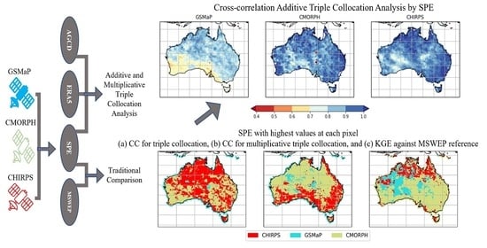
Graphical Abstract

1. Introduction

Precipitation estimates from satellite remote sensing provide an alternative to gauge- or radar-based measurements with greater spatial coverage and improving accuracy [1,2]. Although the Australian Bureau of Meteorology has a well-maintained gauge record dating back decades, satellite precipitation estimates (SPEs) can complement and potentially improve the history of Australian precipitation records, leading to an improved ability to place extreme precipitation events within a climatological context. This leads to better drought and heavy precipitation monitoring [3], amongst numerous other applications [1,4,5,6]. Validation of the accuracy of SPEs is critical to confidence in their usage, but traditionally, this requires a reference dataset that can be taken as ‘truth’, which can be difficult to ascertain, particularly where rain gauges or radar coverage do not exist.
Chua et al. [7] recently performed an analysis of SPEs over Australia that showed that blended satellite-gauge products had higher correlations and smaller errors than a gauge analysis. Beck et al. [8] found that multi-modal SPEs have higher Kling–Gupta efficiency values (KGE) over the continental United States of America (USA) than datasets that were not gauge-corrected. In regions of low gauge density (such as the Tibetan Plateau), sounder-based and gauge-corrected SPEs appear to be more accurate than those that are gauge-calibrated [9]. In addition to the previous findings of SPE comparison over Australia (e.g., [10]), there is yet to be a triple collocation analysis (TCA) using contemporary reference datasets over Australia.
TCA is a technique that is used to calculate metrics of accuracy against numerous independent reference datasets in the absence of a known ‘truth’ [11,12]. Datasets traditionally taken as ‘truth’ such as gauge or even radar data can be lacking in coverage, and in these areas, TCA offers a spatially consistent way of assessing the performance of datasets. Furthermore, the dataset taken as ‘truth’ will always contain its own biases which can skew the analysis. By comparing datasets that ideally have independent errors, TCA helps to circumvent this effect.
There are two models of TCA, depending upon the chosen nature of errors in the SPE. There is an additive error model:
R   =   a + B   T + ϵ
and a multiplicative error model, which is considered more accurate for precipitation data due to the sporadic nature of precipitation amounts [12]:
R = aT b ϵ ,
which can be transformed into
ln R = ln a +   B   ln T +   ln ϵ ,
where R is the observed precipitation amount, T is the unknown true precipitation amount, ϵ is the random error, and a and B denote systematic biases. The multiplicative error model is originally based on a product of the systematic error (aTB) and the random error (ε). The log-normal transformation is introduced to reduce the skewness of the random errors, which are ideally assumed to be normally distributed [13].
The underlying assumptions to perform TCA are: (i) stationarity of the statistics, (ii) linearity between at least three estimates (versus the same target) across all timescales, and (iii) the existence of uncorrelated errors between at least three estimates [11,12]. It should be noted that satisfaction of these assumptions is not just limited to TCA; they are also pertinent for more conventional validation metrics such as the Pearson correlation and the root-mean-squared-error (RMSE) [14].
TCA was originally used to quantify the error characteristics of wind data by Stoffelen (1998) [15]. Roebeling et al. (2012) [16] were the first to apply TCA for precipitation, although contemporary usage is still developing. Wild et al. (2021) [17] previously used the analysis with a reanalysis and soil-moisture-based precipitation estimates over the Pacific Islands to evaluate SPE accuracy without using gauges. Alemohammad et al. (2015) [12] postulated that the multiplicative error model was more realistic for biweekly accumulations in a study over the USA, while Massari et al. (2017) [11] found that usage of the multiplicative error model was unnecessary for daily timescales. Although both studies determined TCA to be an effective means of validation, regional performance should not be generalised due to variation in how the underlying datasets perform over different regions. The investigation of both error models over Australia would be of great value in understanding the applicability of TCA globally, given the wide range of climates in Australia, as well as its variance in density of gauge observations. This study thus aims to address two questions:
  • Is TCA a reasonable validation method for precipitation over Australia?
  • Is the additive or multiplicative error model more appropriate for precipitation TCA over Australia?
The paper is organised as follows: Section 2 describes the study area, datasets, and methods used in the study. Section 3 presents the results, while Section 4 discusses the findings and provides recommendations for SPE usage and comparison. Section 5 summarises the major findings.

2. Materials and Methods

2.1. Study Area and Study Period

The study area of mainland Australia and Tasmania extends from 112.125°E to 155.875°E and 9.875°S to 44.125°S. Only land area was considered. The study period was limited to the range of our SPE data—from January 2001 to December 2020. The data were evaluated on a monthly timescale. Figure 1 provides a map of the study region, along with topography as derived from the ETOPO1 dataset. The ETOPO1 dataset is a 1-arc minute global relief model that models the bedrock and icesheet of the globe through the unification of data from numerous global and regional digital datasets [18]. The locations of stations from December 2020 are also depicted.
The Australian climate spans tropical precipitation in the north with summer monsoons to mid-latitude storms and synoptic-scale frontal systems in the south [19]. The Great Dividing Range causes orographic precipitation off the east coast of the continent, with a desert interior that sporadically experiences precipitation from northwest cloud bands and convective elements. These different precipitation environments lead to variances in SPE performances [20].

2.2. Datasets

For this study, three satellite precipitation datasets widely used in evaluation studies were selected: the Japan Aerospace Exploration Agency’s (JAXA) Global Satellite Mapping of Precipitation (GSMaP V6), the U.S. National Oceanographic and Atmospheric Administration’s (NOAA) Climate Prediction Center morphing technique (CMORPH V1), and Climate Hazards Group’s Infrared Precipitation with Stations (CHIRPS V2).
GSMaP uses the Global Precipitation Mission (GPM) constellation and NOAA Climate Prediction Center (CPC) 4 km infrared (IR) product [21,22]. The version used in this study is the Gauge Near-Real-Time (GNRT) version where the CPC daily global dataset of rain gauges is used to calibrate the GSMaP estimates by roughly matching their values across the past 30 days [9].
In this study, the CMORPH gauge-blended (CMORPH-BLD, hereafter referred to as CMORPH for brevity) product, which further incorporates gauge data through optimal interpolation, was selected for evaluation. It has been shown to be more accurate than its alternative, CMORPH gauge-corrected (CMORPH-CRT), in regions where a dense gauge network exists [7], though performance is similar when gauge density is low [23].
GSMaP and CMORPH data were made available through the WMO’s Space-based Weather and Climate Extremes Monitoring (SWCEM) [24].
The CHIRPS dataset was created as part of the USA Agency for International Development Famine Early Warning Systems Network (FEWS NET) [2]. Compared to similar drought-focused SPEs, CHIRPS performed the best for predicting maize production in Tanzania [25]. It has a higher resolution (0.05°) compared to GSMaP (0.1°) or CMORPH (0.25°) and a larger temporal coverage (beginning from 1981, compared to around the 2000s for other SPEs).
The European Centre for Medium-Range Weather Forecasts (ECMWF) produces the ERA5 reanalysis product, which uses a range of weather observations from multiple sources, including satellites, for humidity, air pressure, wind, and temperature, to provide an accurate history of global meteorology from 1950 to present [26]. It does not directly ingest rain gauge data, with a second-order inclusion occurring from the use of a gauge-adjusted radar analysis over the USA, in the addition to usage of satellite information. Reanalyses were noted to perform better than satellite estimates in Egypt (an arid, gauge-sparse domain) [27], though, over most non-polar latitudes satellite estimates have been demonstrated to be superior [28].
Multi-Source Weighted-Ensemble Precipitation (MSWEP) is a merged product combining numerous gauge, reanalysis, and satellite products [29]. Version 2 of the product provides a higher resolution (0.1°) and corrects to gauges (rather than to the CPC gauge analysis, as CMORPH and GSMaP do). It is considered to be one of the most accurate near-real-time satellite products available due to its optimised merging of other precipitation products [8].
The Australian Gridded Climate Data (AGCD) [30] provides highly accurate rain gauge data, at least where rain gauge density is sufficient, in a gridded format. It is produced by the Australian Bureau of Meteorology (BoM) at a high resolution of 0.05°.
The stations used for verification in this study were obtained from the BoM. Data with a quality flag of less than6 was used, meaning that it had been checked as not being suspect. This resulted in a minimum (maximum) of 4346 (6664) stations across the study period (from 2001 to 2020). These stations are used to create AGCD, leading to in-sample skill inflation during the in situ validation. This also affects CMORPH, CHIRPS, and MSWEP, which are explicitly corrected to a large subset of these stations. GSMaP is less affected because a correction factor based on recent historical values is used, rather than an explicit correction to the value of the current month.
Radar offered a potential validation data source that had the attraction of increased independence to the datasets used in this study. However, we elected not to utilize it because its spatial coverage over Australia is relatively sparse, in addition to it largely overlapping with gauge coverage. An interpolated radar dataset over Australia does not exist. The gaps in radar coverage make it better suited to a study focused on smaller, specific sub-domains, rather than a continental study.
Publicly available datasets are available for ERA5, MSWEP, AGCD, and CHIRPS.

2.3. Method

Python was used for all data handling, verification, and visualization. The NumPy, Matplotlib, and SciPy libraries were used for basic functions, with the triple collocation analysis code being created in line with theory. Data was downloaded as NetCDF4 files for all datasets, converted to units of mm per day, and re-gridded to a common resolution of 0.25° via bilinear interpolation, as this was the coarsest resolution amongst the datasets. A common land–sea mask from CMORPH was applied to all the datasets to remove the variation of masks amongst the datasets. CMORPH’s mask was used as it presented a compromise of coverage between the CHIRPS and ERA5 masks.
The data was segmented into four austral seasons—summer (December, January, and February, hereafter referred to as DJF), autumn (March, April, and May, hereafter referred to as MAM), winter (June, July, and August, hereafter referred to as JJA), and spring (September, October, and November, hereafter referred to as SON).
Three types of validations were performed to evaluate the accuracy of the datasets. The first two were based on the traditional validation method of using a reference dataset. Specifically, these were an in situ comparison to gauges and a comparison to a gridded dataset, MSWEP. The third was a TCA completed by forming triplets between each SPE (GSMaP, CMORPH, and CHIRPS) and the pair of ERA5 and AGCD. Both the additive and multiplicative error models were evaluated.
To perform the in situ comparison, for each station value, a value of the gridded dataset was obtained by re-centering the data to the station location. This was achieved by bilinearly interpolating the gridded data to the coordinates of each station. As a gridded average was compared to a point value, the different sampling scales result in a spatial representation error, but this error would be present across all the datasets, meaning a comparison between datasets is still reasonable.
The Kling–Gupta efficiency (KGE) is a summary statistic that considers the correlation, bias, and variability of a dataset [31]. The KGE was calculated using the stations that were available for each month. The relevant formulae are given below:
KGE = 1 r 1 2 + β 1 2 + γ 1 2
β = μ s μ o   and   γ = σ s / μ s σ o / μ o
where r is the Pearson correlation coefficient, the bias ratio β is the ratio of the estimated and the observed means, and the variability ratio γ is the ratio of the coefficients of variance. The subscripts s and o represent the SPE dataset being verified and the reference dataset, respectively. A KGE value of 1 represents optimal performance or a perfect match to the reference.
The KGE metric was also used for the gridded comparison between GSMaP, CMORPH, CHIRPS, and AGCD to MSWEP. The median of KGE values across each pixel was taken for the gridded analysis, while the KGE was measured month-by-month across all contributing gauges in the study area for the gauge-based analysis due to a differing number of contributing gauges. The bootstrapping (n = 1000) of median values was used to calculate confidence intervals that were visualised on boxplots.
To perform TCA, the time series of the SPEs, AGCD, and ERA5 was used to create a 3 × 3 covariance matrix (C) for each pixel. This matrix was then used to calculate the cross-correlation (CC) and the error statistic (σ) between the SPE and the unknown true precipitation. The equations using an additive error model are:
CC = C X , Y   C X , Z C X , X   C Y , Z
σ = C X , X C X , Y   C X , Z   C Y , Z
where X represents the SPE being considered, Y is AGCD, and Z is ERA5 [11]. Note that these equations can be intuitively explained with the covariance indicating whether the datasets are positively or inversely related to each other. For the CC, the metric improves when the SPE has stronger covariances to AGCD and ERA5 (with the relationship being less significant when AGCD and ERA5 are strongly correlated), and when the variance of the SPE is smaller. For the error statistic, it is proportional to the variance of the SPE, with the second term indicating that the error is smaller when the covariances between the SPE and AGCD and ERA are greater (again, scaled by the covariance of AGCD and ERA5 to indicate lower significance when AGCD and ERA5 are strongly correlated).
Similar equations apply for a multiplicative error model where the time series are converted to a natural logarithmic scale, any values of zero are converted to 0.005 mm/day (the logarithmic function used in the model does not allow for zero values), and the square root is not taken [12].
CC = C X , Y   C X , Z C X , X   C Y , Z
σ = mean X × C X , X C X , Y   C X , Z   C Y , Z
Bootstrapping (n = 500) was used to calculate the 95% confidence interval associated with the values.
Due to the performance of each product varying throughout the year [32], as well as to reduce non-linearity in the datasets from differing climates [14], it is conventional to subtract the climatological average from each month’s value, resulting in the data being expressed as monthly anomalies, rather than totals. However, using anomalies restricts our analysis to the additive error model (Equation (1)) because negative anomaly values in the multiplicative error model would generate imaginary numbers. Consequently, the anomaly approach was not employed in this study and the data maintained its seasonality. Increased non-linearity between the datasets could reduce the statistical significance of the TCA results.

2.4. Evaluation of Satisfaction of Triple Collocation Assumptions

The degree to which the datasets satisfy the assumptions required for TCA is an integral part of this study as it determines how appropriate TCA will be for each dataset. Namely, the assumptions considered in this section are:
  • Linearity between datasets
  • Stationarity of datasets
  • Independence of errors between the datasets

2.4.1. Linearity between Datasets

Each product in the TCA needs to be measuring the same phenomena, and mathematically, TCA relies on the datasets being linearly related. To test this, the anomalies of each dataset are plotted against each other (Figure 2). A high Pearson correlation indicates that the datasets are linearly related.
There is a positive correlation between the SPEs and the reference datasets. GSMaP and CHIRPS both appear to show a greater degree of linearity to ERA5 than to AGCD, whereas CMORPH has stronger linearity to AGCD. There is a temporal trend between CMORPH and ERA5 (middle left) and CHIRPS and AGCD (bottom right), where over time, CMORPH and AGCD show lower values of precipitation values compared to ERA5 and CHIRPS, respectively.

2.4.2. Stationarity of Datasets

The assessment of the stationarity of statistics can be performed with an Augmented Dickey–Fuller Test (ADFT). The smaller the value, the greater the confidence that a dataset is stationary. The probability values correspond to the confidence level in rejecting a null hypothesis that the dataset is not stationary. The results are presented in Table 1.
The total anomaly, as expected, has the greatest confidence of being stationary as it has had the seasonal component subtracted from each month. CMORPH presents unusual results that are inconsistent with the other datasets.

2.4.3. Independence of Errors

Assessing the independence of errors involves the use of a separate reference to act as a truth from which the difference is representative of the error. In this analysis, MSWEP is used as the truth, with the errors being plotted against each other (Figure 3). A high correlation amongst errors would indicate an interdependency between the errors of the datasets.
The plot of CMOPRH and AGCD errors (middle right) shows a strong positive correlation, suggesting an interdependency between the errors of these two datasets. This could be since CMORPH is gauge-blended and AGCD is a gauge analysis, with the strong reliance on gauge data in both resulting in their biases being highly correlated. There does not appear to be any temporal drift in the performance of the datasets.
In general, an interdependency with gauge data across the satellite datasets is expected due to the use of gauges for correction in CMORPH, GSMaP, and CHIRPS. The correlation of the errors suggests this is only problematic for CMORPH, which directly assimilates gauge data, while the other two datasets rely on gauge-based correction factors. ERA5 does not assimilate rainfall data from gauges and so its interdependency with the other datasets in this study is comparatively smaller. A small interdependency with the SPE datasets could be present due to the use of satellite sensors in ERA5 for humidity and cloud information.

2.4.4. Summary

It is evident that GSMaP, CHIRPS, ERA5, and AGCD can form satisfactory triplets with each other. The high correlation of errors between AGCD and CMORPH suggests that TCA metrics will be overinflated for this pairing, and accordingly, some doubt should be placed on this pairing in the TCA.

3. Results

3.1. Gauge Analysis

Table 2 below displays the performance metrics from the in situ comparison. The KGE and the component statistics, as well as the RMSE, are shown, comparing the gridded datasets to the gauge network.
Performance was split into three tiers, with AGCD and MSWEP performing the best, followed by CMORPH and CHIRPS, and lastly by GSMaP. CHIRPS had a slightly better correlation than CMORPH, but after considering the bias and the variance statistic, CMORPH was better. The correlation and bias statistics of CMORPH and CHIRPS were improved compared to GSMaP, but there was little improvement in terms of the variance, which appeared to be the most problematic statistic among the three.
GSMaP was the only dataset to demonstrate a median bias ratio of below one. However, the mean bias ratios (not shown for brevity) were all lower, with all the satellite datasets being below one. Given that the mean is more sensitive to outliers than the median, this suggests that although the datasets generally tended to overestimate, the outliers were cases of underestimation.

3.2. Gridded Analysis

Table 3 and Figure 4 summarise the findings from the comparison to MSWEP. The same statistics from Table 2 were used to provide a comparison of performance.
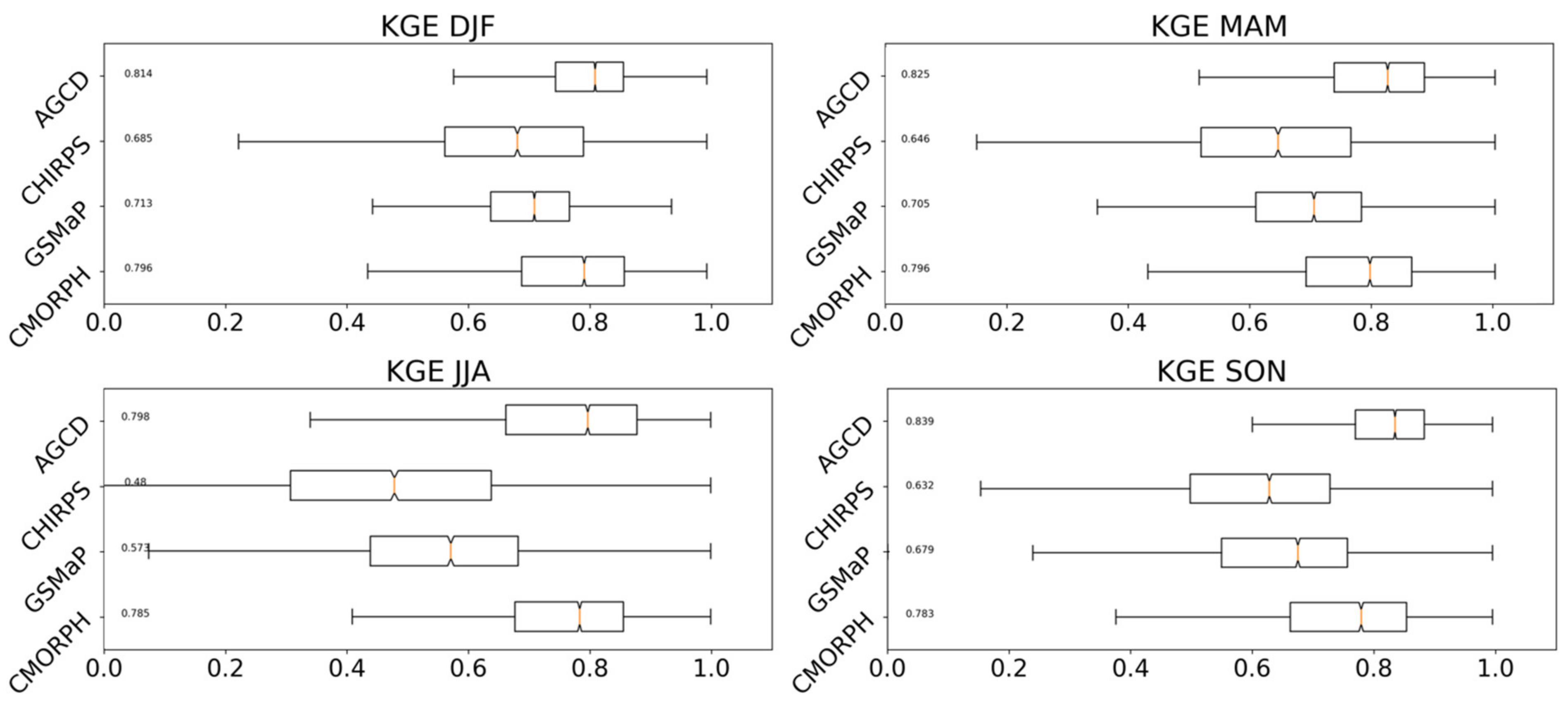
Using MSWEP as the truth resulted in GSMaP obtaining a better KGE than CHIRPS. The ranking of the other datasets remained the same compared to the in situ comparison, though the superiority of AGCD over CMORPH was greatly reduced. The variance ratio for GSMaP and CMORPH was greater than for the in situ validation, while CHIRPS consistently underestimated the variance. SPE performance across the seasons followed similar trends, with CMORPH obtaining the best metrics, followed by CHIRPS and then GSMaP. All four products performed more poorly during JJA. The spatial variation of the RMSEs is visualized in Figure 5.
The RMSE for all the datasets is greatest over northern Australia, likely related to the large rainfall totals in that region over JJA. CHIRPS and GSMaP also display noticeable RMSEs over western Tasmania, while large RMSEs also exist along the eastern coast of Australia for GSMaP.

3.3. Collocation Analysis

Table 4 summarizes the results from the TCA. The spatial distribution of the highest values in each pixel is displayed in Figure 6.
The different error models yield some differences in the ranking of the datasets. Primarily, if M CC is considered, then CMORPH is the most performant; otherwise, the other metrics suggest CHIRPS is the most performant. GSMaP is the least performant of the three. This has similarities to the traditional comparisons where GSMaP had inferior values of RMSE and Pearson correlations in both the in situ and MSWEP validations. CMORPH is the dataset with the most direct correction to gauge data, and, generally, it is the most performant dataset where gauge density is relatively high. GSMaP has a greater presence over the gauge-sparse interior, while CHIRPS seems to perform well over northern Australia, which could be related to better performance for rainfall from tropical modes or that which occurs at heavier intensities. Figure 7 shows the spatial distribution of the CC from the triple collocation.
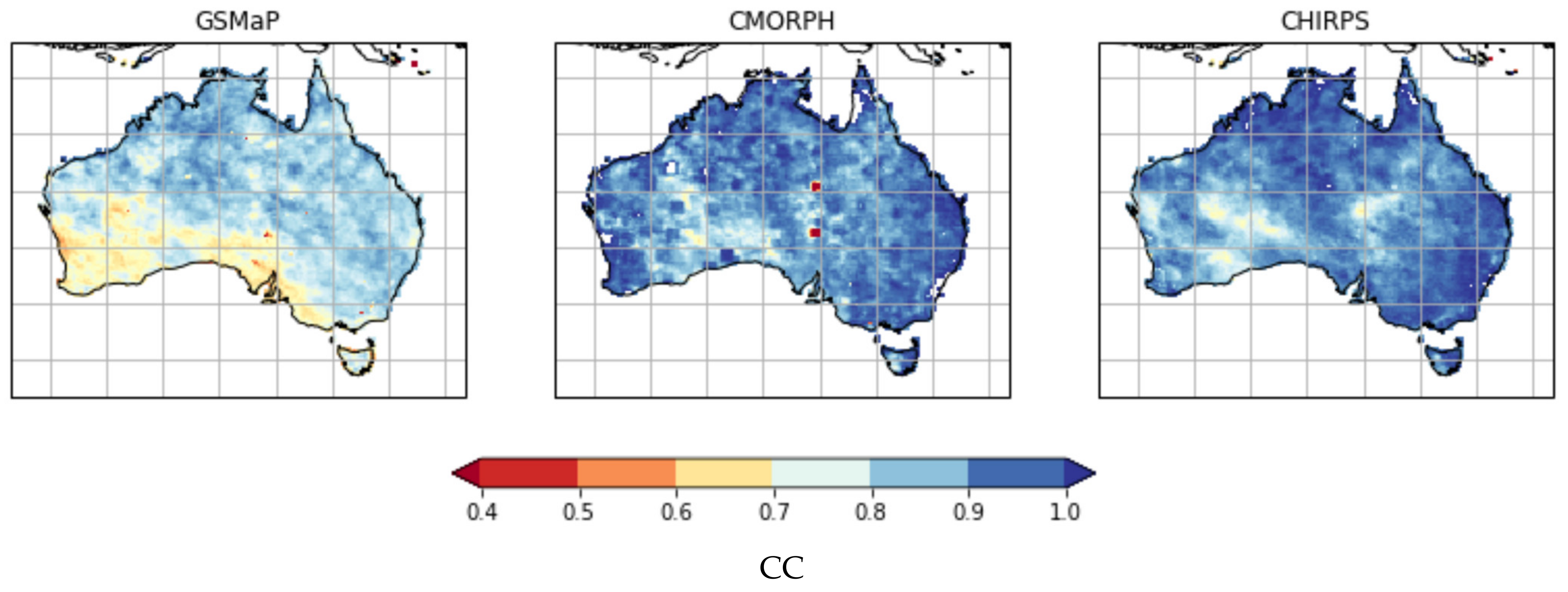
The CCs of the satellite datasets are lowest over southwest Australia while being higher over northern and southeast Australia. There are two spots of very low CC in CMORPH over the interior of the mainland, which could be from the assimilation of poor station data.

4. Discussion

4.1. Dataset Deficiencies

The gridded datasets were expected to underestimate the variance in both the frequency and amount of precipitation [33]; indeed, AGCD was under-dispersed, as well. However, the satellite datasets presented additional under-dispersion that could not be rectified by gauge correction, at least by the techniques used to create CMORPH and CHIRPS. The marked superiority of MSWEP over the satellite datasets indicates the effectiveness of its correction and merging techniques, though some of this improvement would be due to in-sample inflation, with MSWEP being directly corrected to a large subset of the BoM stations.
The KGE of CHIRPS was lower in the gridded comparison than in the in situ comparison, falling behind GSMaP. The use of gridded data as truth removes spatial representativeness error, and thus performance was expected to increase. It appears this performance increase was outweighed by other factors. It suggests that although CHIRPS has good performance close to stations, its performance when gauge density is low is relatively poor, as seen in Figure 5. The results support previous results by Nashwan et al. (2020) [34] that GSMaP is more accurate in gauge-sparse areas than CHIRPS; however, the higher CC values of CHIRPS in TCA with ERA5 were also observed in Pacific Islands by Wild et al. (2021) [17].
All the datasets displayed less variability in precipitation amount and frequency than MSWEP, but this was particularly problematic in CHIRPS. The variability for areas and periods of very low precipitation, such as JJA over northern Australia, was severely underestimated.

4.2. How Does TCA Compare to Traditional Verification Methods of Precipitation over Australia?

The value of TCA is not necessarily in the absolute metrics obtained, which varies with the datasets used to make the data triplet. Instead, it has great value in providing information on the relative ranking of datasets. Compared to the in situ comparison, the TCA results were similar.
In terms of the correlation, CMORPH and CHIRPS performed noticeably better than GSMaP, which was reflected in all the validations. However, CMORPH outperformed CHIRPS in the gauge and gridded comparison, while the converse occurred in the additive triple collocation, albeit marginally. The rankings obtained from the multiplicative triple collocation matched the other validations. In the gridded comparison, even though the KGE indicated GSMaP was better, it is reassuring that ranking the datasets via the Pearson correlations yielded CHIRPS as better, in line with the TCA.
When the RMSE was considered, the ranking of the datasets was the same for all the verifications with CHIRPS performing the best, followed by CMORPH and then GSMaP. The difference between CHIRPS and CMORPH was slight for the in situ and gridded comparisons.
One metric which does not match so well with the traditional comparisons is the multiplicative triple collocation error σ. Even though the ranking matched those obtained in the other validations, it indicated that CHIRPS was significantly better than CMORPH, a finding not supported by the other validations. This seemed to be a combination of both an exaggeration of the performance of CHIRPS and an underestimation of CMORPH’s.
Figure 6 demonstrates that in the gridded validation, CMORPH performed the best overall, with CHIRPS performing the best over northern Australia and western Tasmania and GSMaP performing the best over regions with very low gauge densities. This pattern was also observed in the additive triple collocation, though the performance of CHIRPS was overestimated and that of GSMaP was underestimated relative to MSWEP. The multiplicative triple collocation did not match this pattern and presented an almost inverse result, with CHIRPS being superior over southern Australia, the Queensland coast, and eastern Tasmania. The representation of GSMaP was slightly better but still underestimated.
Figure 7 demonstrates noticeable areas that have reduced CCs. Some of these areas have low gauge density (i.e., the interior parts of South Australia and Western Australia), resulting in greater uncertainty in the datasets that can manifest as a reduction in skill. For the remaining regions of GSMaP that have lower CCs but reasonable gauge density (i.e., the southwest-facing coastal parts of Western Australia and South Australia), this could be an allusion to a known deficiency of satellite datasets having difficulty with representing precipitation from cold fronts [7]. The other two SPE datasets have a higher degree of gauge correction, which alleviates this issue and leads to their higher CCs in these areas. If this is the case, the apparent ability of TCA to detect these areas where reductions in performances are expected is supportive of its value.
As mentioned in Section 2.4.3, the relatively high interdependence between the errors of CMORPH and AGCD weakens the robustness of this pairing in TCA, likely leading to an inflation of skill. The traditional validations also placed CMORPH as the best SPE dataset, but they would be afflicted by this interdependency as well.
Even though the dataset rankings from the overall correlation slightly favor multiplicative triple collocation, the greater discrepancy in the error results, along with the spatial correlation pattern, suggests that additive triple collocation was more consistent with traditional verification methods in this study. This result is consistent with [11], which found that on a daily scale (and by inference, for coarser scales as well), additive TCA produced reasonable and robust results, with no advantage gained from using the multiplicative version. In contrast, some previous studies found the multiplicative error model to be more accurate than the additive model [12,13]. However, those studies also examined precipitation on smaller timescales (daily and biweekly respectively compared to monthly in this study) where the more irregular nature of the precipitation amounts may have lent itself better to the multiplicative model.

5. Conclusions

The estimation of precipitation is of great value to society, and in the modern era, it can be conducted through a number of methods. These methods are broadly categorized into those based on satellite, model reanalyses, and rain gauges. Within these three sources, an even greater number of algorithms exist, resulting in a multitude of precipitation datasets. The accurate verification of these datasets enables users to select the dataset which is the most performant.
Traditional verification relies heavily on comparison to rain gauges, but the effectiveness of this declines sharply when gauge density becomes low. Triple collocation analysis (TCA) presents an alternative that ranks datasets based on their coherence as a set of three independent datasets. This study investigated the effectiveness of TCA for precipitation estimates over Australia by comparing three satellite datasets (GSMaP, CMORPH and CHIRPS) to ERA5 and AGCD. Both the additive and multiplicative versions of TCA were employed.
The multiplicative TCA gave correlation rankings that matched two traditional forms of validations, whereas, in the additive version the order of CMORPH and CHIRPS was reversed. However, the correlations of these two datasets were similar amongst all the verifications, making a reversal in the order of these two datasets a reasonable discrepancy. A greater disparity was observed in the multiplicative TCA error, where although the dataset rankings were the same as the other validations, the performance of CHIRPS appeared to be significantly overinflated while that of CMORPH was underestimated. Additionally, the additive TCA had a better match, spatially, to that of MSWEP compared to its multiplicative counterpart.
The additive TCA showed better skill scores than the multiplicative version for monthly precipitation verification over Australia. Overall, apart from the multiplicative TCA errors, the results obtained via TCA were largely consistent with those from the gridded and the in situ comparison both in terms of ranking and relative performance. This demonstrates the value of TCA in assessing the performance of datasets, especially over data-sparse regions, though care must be taken to ensure that the requisite assumptions are met.

Author Contributions

Conceptualization, A.W. and Y.K.; methodology, A.W.; software, A.W. and Z.-W.C.; validation, A.W.; formal analysis, Z.-W.C.; investigation, Z.-W.C.; writing—original draft preparation, A.W. and Z.-W.C.; writing—review and editing, A.W., Z.-W.C. and Y.K.; supervision, Y.K.; project administration, Y.K.; funding acquisition, Y.K. All authors have read and agreed to the published version of the manuscript.

Funding

This research received no external funding.

Data Availability Statement

GSMaP data were provided by JAXA (access can be sought from https://sharaku.eorc.jaxa.jp/GSMaP/registration.html); CMORPH, by CPC, NOAA (https://www.ncei.noaa.gov/data/cmorph-high-resolution-global-precipitation-estimates/); CHIRPS, by FEWS NET (https://data.chc.ucsb.edu/products/CHIRPS-2.0/); MSWEP, by GloH2O (access can be sought from http://www.gloh2o.org/); and ERA5, by ECMWF (https://www.ecmwf.int/en/forecasts/datasets/reanalysis-datasets/era5). This study contains modified Copernicus Climate Change Service Information (2019). Neither the European Commission nor ECMWF is responsible for any use that may be made of the Copernicus Information or the data it contains.

Acknowledgments

We are grateful to colleagues from the Bureau of Meteorology and Monash University for their helpful advice and guidance.

Conflicts of Interest

The authors declare no conflict of interest.

Abbreviations

ADFTAugmented Dickey–Fuller Test
AGCDAustralian Gridded Climate Dataset
BOMBureau of Meteorology
CCCorrelation co-efficient
CHIRPSClimate Hazards Group Infrared Precipitation with Stations
CMORPH-BLDClimate Prediction Center morphing technique (Blended)
CMORPH-CRTClimate Prediction Center morphing technique (Corrected)
CPCClimate Prediction Center
DJFDecember, January, and February
ECMWFEuropean Centre for Medium-Range Weather Forecasts
ERA5Fifth-generation ECMWF reanalysis
FEWS NETFamine Early Warning Systems Network
GSMaPGlobal Satellite Mapping of Precipitation
GSMaP-GNRTGlobal Satellite Mapping of Precipitation (Gauge Near Real-time Adjusted)
JAXAJapan Aerospace Exploration Agency
JJAJune, July, and August
KGEKling–Gupta efficiency
MAMMarch, April, and May
MSWEPMulti-Source Weighted-Ensemble Precipitation
NOAANational Oceanographic and Atmospheric Administration
RMSERoot-mean-squared-error
SONSeptember, October, and November
SPESatellite precipitation estimate
TCATriple collocation analysis
USAUnited States of America
Var. ratioVariance ratio

References

  1. Dinku, T. The Value of Satellite Rainfall Estimates in Agriculture and Food Security. In Satellite Precipitation Measurement; Advances in Global Change Research; Springer: Cham, Switzerland, 2020; pp. 1113–1129. [Google Scholar]
  2. Funk, C.; Peterson, P.; Landsfeld, M.; Pedreros, D.; Verdin, J.; Shukla, S.; Husak, G.; Rowland, J.; Harrison, L.; Hoell, A.; et al. The climate hazards infrared precipitation with stations—A new environmental record for monitoring extremes. Sci. Data 2015, 2, 150066. [Google Scholar] [CrossRef] [Green Version]
  3. Tarnavsky, E.; Bonifacio, R. Drought Risk Management Using Satellite-Based Rainfall Estimates. In Satellite Precipitation Measurement; Advances in Global Change Research; Springer: Cham, Switzerland, 2020; pp. 1029–1053. [Google Scholar]
  4. Li, X.; Chen, Y.; Deng, X.; Zhang, Y.; Chen, L. Evaluation and Hydrological Utility of the GPM IMERG Precipitation Products over the Xinfengjiang River Reservoir Basin, China. Remote Sens. 2021, 13, 866. [Google Scholar] [CrossRef]
  5. Stanley, T.; Kirschbaum, D.B.; Pascale, S.; Kapnick, S. Extreme Precipitation in the Himalayan Landslide Hotspot. In Satellite Precipitation Measurement; Advances in Global Change Research; Springer: Cham, Switzerland, 2020; pp. 1087–1111. [Google Scholar]
  6. LeRoy, A.; Berndt, E.; Molthan, A.; Zavodsky, B.; Smith, M.; LaFontaine, F.; McGrath, K.; Fuell, K. Operational Applications of Global Precipitation Measurement Observations. In Satellite Precipitation Measurement; Advances in Global Change Research; Springer: Cham, Switzerland, 2020; pp. 919–940. [Google Scholar]
  7. Chua, Z.-W.; Kuleshov, Y.; Watkins, A. Evaluation of Satellite Precipitation Estimates over Australia. Remote Sens. 2020, 12, 678. [Google Scholar] [CrossRef] [Green Version]
  8. Beck, H.E.; Pan, M.; Roy, T.; Weedon, G.P.; Pappenberger, F.; van Dijk, A.I.J.M.; Huffman, G.J.; Adler, R.F.; Wood, E.F. Daily evaluation of 26 precipitation datasets using Stage-IV gauge-radar data for the CONUS. Hydrol. Earth Syst. Sci. 2019, 23, 207–224. [Google Scholar] [CrossRef] [Green Version]
  9. Lu, D.; Yong, B. Evaluation and Hydrological Utility of the Latest GPM IMERG V5 and GSMaP V7 Precipitation Products over the Tibetan Plateau. Remote Sens. 2018, 10, 2022. [Google Scholar] [CrossRef] [Green Version]
  10. Ebert, E.E.; Janowiak, J.E.; Kidd, C. Comparison of Near-Real-Time Precipitation Estimates from Satellite Observations and Numerical Models. Bull. Am. Meteorol. Soc. 2007, 88, 47–64. [Google Scholar] [CrossRef] [Green Version]
  11. Massari, C.; Crow, W.; Brocca, L. An assessment of the performance of global rainfall estimates without ground-based observations. Hydrol. Earth Syst. Sci. 2017, 21, 4347–4361. [Google Scholar] [CrossRef] [Green Version]
  12. Alemohammad, S.H.; McColl, K.A.; Konings, A.G.; Entekhabi, D.; Stoffelen, A. Characterization of precipitation product errors across the United States using multiplicative triple collocation. Hydrol. Earth Syst. Sci. 2015, 19, 3489–3503. [Google Scholar] [CrossRef] [Green Version]
  13. Tian, Y.; Huffman, G.J.; Adler, R.F.; Tang, L.; Sapiano, M.; Maggioni, V.; Wu, H. Modeling errors in daily precipitation measurements: Additive or multiplicative? Geophys. Res. Lett. 2013, 40, 2060–2065. [Google Scholar] [CrossRef] [Green Version]
  14. Gruber, A.; Su, C.-H.; Zwieback, S.; Crow, W.; Dorigo, W.; Wagner, W. Recent advances in (soil moisture) triple collocation analysis. Int. J. Appl. Earth Obs. Geoinf. 2016, 45, 200–211. [Google Scholar] [CrossRef]
  15. Stoffelen, A. Toward the true near-surface wind speed: Error modeling and calibration using triple collocation. J. Geophys. Res. Ocean. 1998, 103, 7755–7766. [Google Scholar] [CrossRef]
  16. Roebeling, R.A.; Wolters, E.L.A.; Meirink, J.F.; Leijnse, H. Triple Collocation of Summer Precipitation Retrievals from SEVIRI over Europe with Gridded Rain Gauge and Weather Radar Data. J. Hydrometeorol. 2012, 13, 1552–1566. [Google Scholar] [CrossRef]
  17. Wild, A.; Chua, Z.-W.; Kuleshov, Y. Evaluation of Satellite Precipitation Estimates over the South West Pacific Region. Remote Sens. 2021, 13, 3929. [Google Scholar] [CrossRef]
  18. Amante, C.; Eakins, B.W. ETOPO1 1 Arc-Minute Global Relief Model: Procedures, Data Sources and Analysis. In NOAA Technical Memorandum NESDIS NGDC-24; US Department Commerce: Boulder, CO, USA, 2009. [Google Scholar] [CrossRef]
  19. Masunaga, H.; Schröder, M.; Furuzawa, F.A.; Kummerow, C.; Rustemeier, E.; Schneider, U. Inter-product biases in global precipitation extremes. Environ. Res. Lett. 2019, 14, 125016. [Google Scholar] [CrossRef]
  20. Prat, O.P.; Nelson, B.R. Satellite Precipitation Measurement and Extreme Rainfall. In Satellite Precipitation Measurement; Advances in Global Change Research; Springer: Cham, Switzerland, 2020; pp. 761–790. [Google Scholar]
  21. Tashima, T.; Kubota, T.; Mega, T.; Ushio, T.; Oki, R. Precipitation Extremes Monitoring Using the Near-Real-Time GSMaP Product. IEEE J. Sel. Top. Appl. Earth Obs. Remote Sens. 2020, 13, 5640–5651. [Google Scholar] [CrossRef]
  22. Kubota, T.; Aonashi, K.; Ushio, T.; Shige, S.; Takayabu, Y.N.; Kachi, M.; Arai, Y.; Tashima, T.; Masaki, T.; Kawamoto, N.; et al. Global Satellite Mapping of Precipitation (GSMaP) Products in the GPM Era. In Satellite Precipitation Measurement; Advances in Global Change Research; Springer: Cham, Switzerland, 2020; pp. 355–373. [Google Scholar]
  23. Chua, Z.-W.; Kuleshov, Y.; Watkins, A.B. Drought Detection over Papua New Guinea Using Satellite-Derived Products. Remote Sens. 2020, 12, 3859. [Google Scholar] [CrossRef]
  24. Kuleshov, Y.; Kurino, T.; Kubota, T.; Tashima, T.; Xie, P. WMO Space-based Weather and Climate Extremes Monitoring Demonstration Project (SEMDP): First Outcomes of Regional Cooperation on Drought and Heavy Precipitation Monitoring for Australia and Southeast Asia. In Rainfall-Extremes, Distribution and Properties; IntechOpen: London, UK, 2019; pp. 51–57. [Google Scholar]
  25. Tarnavsky, E.; Chavez, E.; Boogaard, H. Agro-meteorological risks to maize production in Tanzania: Sensitivity of an adapted Water Requirements Satisfaction Index (WRSI) model to rainfall. Int. J. Appl. Earth Obs. Geoinf. 2018, 73, 77–87. [Google Scholar] [CrossRef]
  26. Hersbach, H.; Bell, B.; Berrisford, P.; Hirahara, S.; Horányi, A.; Muñoz-Sabater, J.; Nicolas, J.; Peubey, C.; Radu, R.; Schepers, D.; et al. The ERA5 global reanalysis. Q. J. R. Meteorol. Soc. 2020, 146, 1999–2049. [Google Scholar] [CrossRef]
  27. Hamed, M.M.; Nashwan, M.S.; Shahid, S. Performance evaluation of reanalysis precipitation products in Egypt using fuzzy entropy time series similarity analysis. Int. J. Climatol. 2021, 41, 5431–5446. [Google Scholar] [CrossRef]
  28. Tang, G.; Clark, M.P.; Papalexiou, S.M.; Ma, Z.; Hong, Y. Have satellite precipitation products improved over last two decades? A comprehensive comparison of GPM IMERG with nine satellite and reanalysis datasets. Remote Sens. Environ. 2020, 240, 111697. [Google Scholar] [CrossRef]
  29. Beck, H.E.; van Dijk, A.I.J.M.; Levizzani, V.; Schellekens, J.; Miralles, D.G.; Martens, B.; de Roo, A. MSWEP: 3-hourly 0.25° global gridded precipitation (1979–2015) by merging gauge, satellite, and reanalysis data. Hydrol. Earth Syst. Sci. 2017, 21, 589–615. [Google Scholar] [CrossRef] [Green Version]
  30. Evans, A.; Jones, D.; Smalley, R.; Lellyett, S. An Enhanced Gridded Rainfall Dataset Scheme for Australia; Bureau of Meteorology: Melbourne, Australia, 2020; ISBN 978-1-925738-12-4.
  31. Kling, H.; Fuchs, M.; Paulin, M. Runoff conditions in the upper Danube basin under an ensemble of climate change scenarios. J. Hydrol. 2012, 424–425, 264–277. [Google Scholar] [CrossRef]
  32. Chen, F.; Crow, W.T.; Ciabatta, L.; Filippucci, P.; Panegrossi, G.; Marra, A.C.; Puca, S.; Massari, C. Enhanced Large-Scale Validation of Satellite-Based Land Rainfall Products. J. Hydrometeorol. 2021, 22, 245–257. [Google Scholar] [CrossRef]
  33. Robeson, S.M.; Ensor, L.A. Statistical Characteristics of Daily Precipitation: Comparisons of Gridded and Point Datasets. J. Appl. Meteorol. Climatol. 2008, 47, 2468–2476. [Google Scholar] [CrossRef]
  34. Nashwan, M.S.; Shahid, S.; Dewan, A.; Ismail, T.; Alias, N. Performance of five high resolution satellite-based precipitation products in arid region of Egypt: An evaluation. Atmos. Res. 2020, 236, 104809. [Google Scholar] [CrossRef]
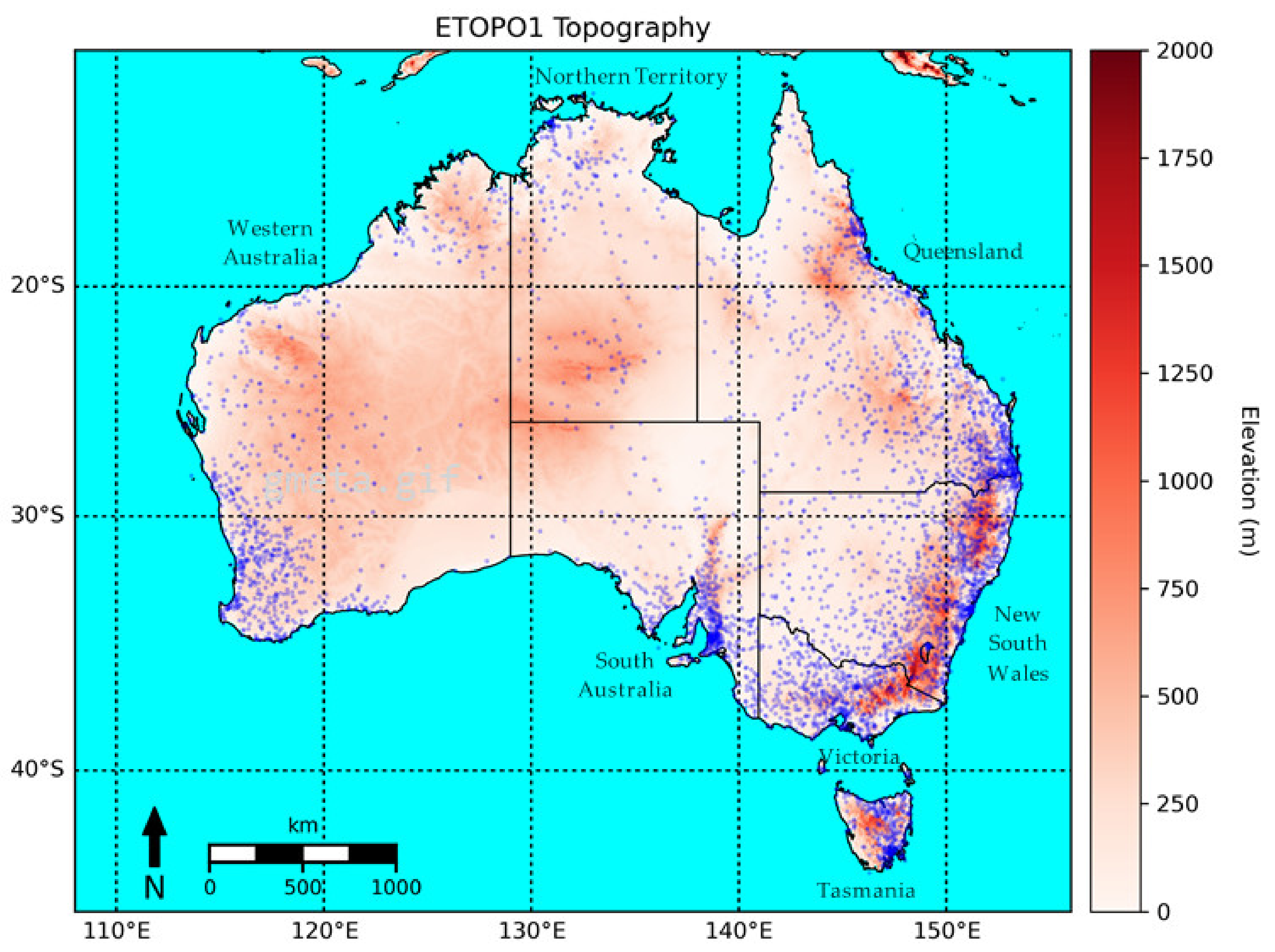
Figure 1. Map of study domain, adapted from [7]. The blue dots represent stations, while the white–red shading depicts elevation as derived from the ETOPO1 dataset.
Remotesensing 14 02724 g001
Figure 2. Scatterplot of monthly average precipitation anomalies across the study region for each SPE compared to ERA5 and AGCD. Units are in mm/day. The pale dots indicate months earlier in the study period and the dark dots represent months closer to the end of the study period.
Remotesensing 14 02724 g002
Figure 3. Scatterplot of monthly average precipitation errors (dataset minus MSWEP) across the study region for each SPE compared to ERA5 and AGCD. Units are in mm/day. The pale dots indicate months earlier in the study period and the dark dots represent months closer to the end of the study period.
Remotesensing 14 02724 g003
Figure 4. Boxplots showing the distribution of the Kling–Gupta efficiency (KGE) between SPEs and AGCD with MSWEP for each season. Outliers are not included within the boxplots to improve clarity. The median value (orange line) is shown on the left of each plot.
Remotesensing 14 02724 g004
Figure 5. RMSE errors for comparing each dataset to MSWEP across all seasons. Lower values indicate better performance.
Remotesensing 14 02724 g005
Figure 6. Distribution of pixels with highest (a) CC for triple collocation, (b) CC for multiplicative triple collocation, and (c) KGE against MSWEP reference.
Remotesensing 14 02724 g006
Figure 7. CC metrics between each SPE with AGCD and ERA5. Higher values indicate better performance.
Remotesensing 14 02724 g007
Table 1. Augmented Dickey–Fuller Test results for each season, as well as the score for significance.
DatasetRawAnomalyDJFMAMJJASON
GSMaP−3.16 *−6.75 **−5.76 **−3.09 *−7.30 **−2.42
CMORPH−2.46−2.43−2.23−2.46−1.08−2.00
CHIRPS−3.18 *−8.20 **−3.56 **−3.95 **−7.19 **−2.38
ERA5−1.52−6.22 **−1.53−1.53−1.53−1.52
AGCD−2.55−2.64 *−6.54 **−3.67 **−6.84 **−2.14
The symbols * and ** are used to denote p < 0.10 and p < 0.05, respectively.
Table 2. Median KGE (as well its components), along with the RMSE, across the study period.
GSMaPCMORPHCHIRPSAGCDMSWEP
KGE0.5870.8080.7410.9330.871
Pearson0.7270.9170.9030.9800.944
Bias Ratio0.9721.0671.1081.0221.071
Var. Ratio0.8470.8970.8360.9450.945
RMSE1.3910.8560.8370.3710.623
Table 3. Medians for the values at each pixel across the study area.
GSMaPCMORPHCHIRPSAGCD
KGE0.7430.8350.7080.861
Pearson0.8150.9150.8870.906
Bias Ratio1.0161.0760.9730.998
Variance Ratio0.9900.9970.7870.990
RMSE0.7890.6400.6470.570
Table 4. Medians for the values at each pixel across the study area. M CC and M σ refer to the TCA metrics when the multiplicative error model was used.
GSMaPCMORPHCHIRPS
CC0.8390.9290.932
M CC0.6680.7960.748
σ0.6470.5270.329
M σ1.9881.5370.169
Publisher’s Note: MDPI stays neutral with regard to jurisdictional claims in published maps and institutional affiliations.