Article

Landslide Susceptibility Mapping Based on the Germinal Center Optimization Algorithm and Support Vector Classification

1
Faculty of Engineering, China University of Geosciences, Wuhan 430074, China
2
Badong National Observation and Research Station of Geohazards, China University of Geosciences, Wuhan 430074, China
*
Author to whom correspondence should be addressed.
Remote Sens. 2022, 14(11), 2707; https://doi.org/10.3390/rs14112707
Submission received: 17 April 2022 / Revised: 27 May 2022 / Accepted: 2 June 2022 / Published: 4 June 2022

Abstract

:
A landslide susceptibility model based on a metaheuristic optimization algorithm (germinal center optimization (GCO)) and support vector classification (SVC) is proposed and applied to landslide susceptibility mapping in the Three Gorges Reservoir area in this paper. The proposed GCO-SVC model was constructed via the following steps: First, data on 11 influencing factors and 292 landslide polygons were collected to establish the spatial database. Then, after the influencing factors were subjected to multicollinearity analysis, the data were randomly divided into training and testing sets at a ratio of 7:3. Next, the SVC model with 5-fold cross-validation was optimized by hyperparameter space search using GCO to obtain the optimal hyperparameters, and then the best model was constructed based on the optimal hyperparameters and training set. Finally, the best model acquired by GCO-SVC was applied for landslide susceptibility mapping (LSM), and its performance was compared with that of 6 popular models. The proposed GCO-SVC model achieved better performance (0.9425) than the genetic algorithm support vector classification (GA-SVC; 0.9371), grid search optimized support vector classification (GRID-SVC; 0.9198), random forest (RF; 0.9085), artificial neural network (ANN; 0.9075), K-nearest neighbor (KNN; 0.8976), and decision tree (DT; 0.8914) models in terms of the area under the receiver operating characteristic curve (AUC), and the trends of the other metrics were consistent with that of the AUC. Therefore, the proposed GCO-SVC model has some advantages in LSM and may be worth promoting for wide use.

1. Introduction

Landslides are the most common geological disaster, and they have wide distributions, pose a high risk, and cause serious damage [1,2]. Many internal and external factors contribute to landslide occurrence, including topographic, geological, hydrological, seismic, and surface factors and factors associated with human engineering activity [3,4]. Thus, landslide spatial prediction based on these influencing factors, which is also called landslide susceptibility mapping (LSM), is important for preventing and reducing landslide damage [5].
In recent years, various machine learning methods have been applied for regional LSM, including artificial neural network (ANN) [6,7,8,9], random forest (RF) [10,11], decision tree (DT) [12,13], logistic regression (LR) [14], K-nearest neighbor (KNN) [15,16], extreme learning machine (ELM) [17], and support vector machine (SVM) models [18,19]. Machine learning models are popular, mature, and promising for LSM. For example, SVM models are widely used in LSM due to their powerful generalization ability on small samples [7,13]. However, such deep learning models generally have many hyperparameters, which directly affect the model results [20,21]. Therefore, it is extremely important that these models choose the appropriate combination of hyperparameters for LSM.
To solve this problem, many algorithms have been used to perform hyperparameter optimization of deep learning models [22,23]. One of the most commonly used algorithms is the violent grid search algorithm [12,24], which iterates through all combinations of the listed hyperparameters and scores them to select the best hyperparameters. The process may be effective for finite discrete space search, but exhaustive enumeration for continuous hyperparameter space is almost impossible. Therefore, metaheuristic algorithms have recently been applied and are increasingly used in model hyperparameter optimization, with the most applied algorithms being genetic algorithms (GAs) [25,26] and particle swarm optimization algorithms [27]. It has been demonstrated that the optimization of model hyperparameters for LSM results is enhanced by the use of metaheuristic algorithms.
In this study, a new model named GCO-SVC was proposed and applied to LSM in the Zigui to Badong basins of the Three Gorges Reservoir area (TGRA). This effort represents the first application of the metaheuristic germinal center optimization (GCO) algorithm to the hyperparameter optimization of the SVC model and its use for LSM. To validate the proposed model, six popular models, artificial neural network (ANN), decision tree (DT), K-nearest neighbor (KNN), random forest (RF), grid search optimized support vector classification (GRID-SVC), and genetic algorithm optimized support vector classification (GA-SVC), and four common metrics, namely accuracy, F1 score, Log loss, and area under the receiver operating characteristic curve (AUC), were employed for comparative study.

2. Methods

This study consists of four main steps, as shown in Figure 1: (1) data collection, including the landslide inventory map and influencing factors; (2) dataset preparation and landslide influencing factor analysis; (3) spatial prediction modeling of landslides using the proposed GCO-SVC and six other models; and (4) model performance evaluation based on multiple statistical tools.

2.1. Study Area

2.1.1. Description of the Study Area

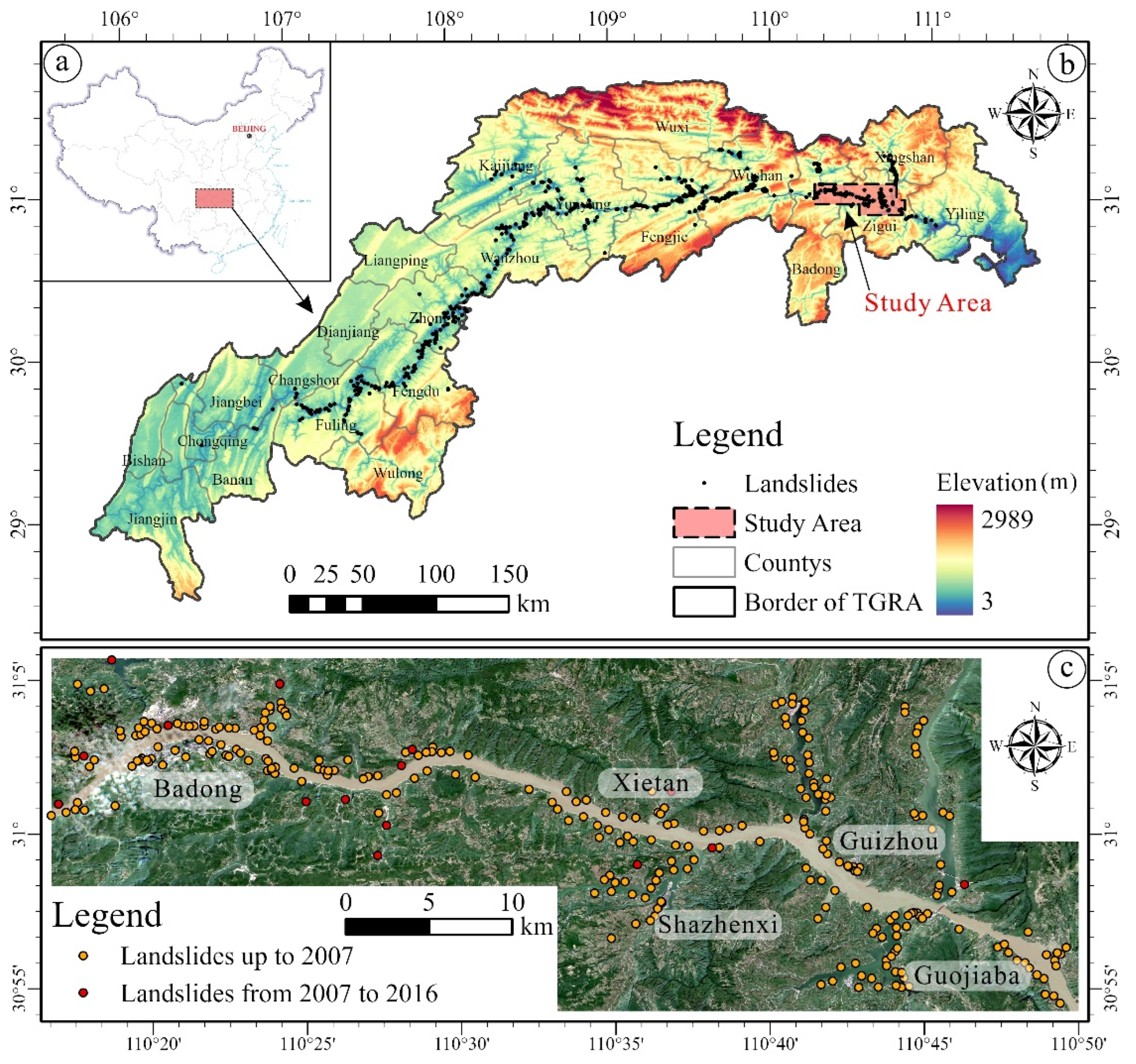
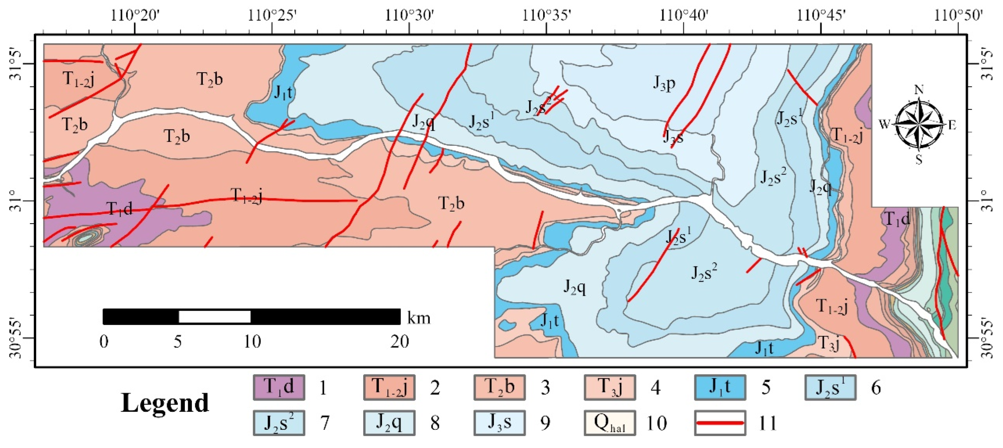
The study area is located in Hubei Province, China. It belongs to the Zigui to Badong basins of the TGRA, within longitudes 110°15′~110°50′ east and latitudes 30°50′~1°6′ north, and the total area is approximately 900 km2 (Figure 2). In total, 4256 landslides and rock avalanches with a total volume of roughly 4.24 billion m3 have been found in the TGRA [1]; those in the study area account for 16% of the total. The average annual rainfall is 1100–1200 mm, and most of the precipitation is concentrated from April to September [28]. This study area is a Mesozoic tectonic basin that developed and was shaped in the Late Triassic–Early Jurassic period, and it is mainly composed of Jurassic terrestrial and Middle–Upper Triassic coastal-phase clastic rocks (Figure 3). The primary strata that crop out in this area include the Triassic Jialingjiang (T1-2j) and Badong (T2b) formations and the Jurassic Qianfoya (J2q), Shaximiao (J2s), and Suining (J3s) formations.
In recent years, the construction and impoundment of the Three Gorges Dam have led to increased numbers of engineering activities along the Yangtze River in the area, such as urban relocation and reconstruction and road and high-speed railway construction, which have had significant impacts on the engineering geological environment and led to frequent geological hazards in the area. Moreover, the periodic reservoir water level and seasonal rainfall exacerbate the landslide geological hazards in this area [29].

2.1.2. Landslide Inventory

For LSM, the first important step is to acquire the exact locations of landslides that have occurred [30]. The landslide distribution up to 2016 in the study area was obtained by compiling data from field surveys, satellite images, and a literature review, as shown in Figure 2c. The landslide distribution prior to 2007 was provided by the Three Gorges Reservoir Area Geological Disaster Prevention and Control Work Command (TGWC), while the landslides from 2007 to 2016 were determined by the authors based on open-source data [31], Google Maps, and Sentinel-2B images. In 2016, a total of 292 landslides were identified in the study area, with a total area of 32.43 km2, accounting for 8.11% of the whole study area, and Quaternary deposit landslides and rock landslides were found to be the main types [32]. For large-scale LSM, landslide inventories are usually compiled with point data to improve mapping efficiency, avoid uncertainty in the description of landslide boundaries, decrease spatial autocorrelation across landslides, and treat landslides of different scales equally [33,34,35].

2.1.3. Influencing Factors

Landslide hazards are usually triggered by a combination of internal geological conditions and external environmental factors. Many previous studies [18,36] in the TGRA have indicated that landslides in this area are primarily influenced by hydrological conditions and human engineering activities, as well as by their own geological conditions. Therefore, a digital elevation model (DEM), geologic map, road network, river network, rainfall monitoring, and land use data were compiled from previous studies [11,32] and field investigations, and their sources and descriptions are provided in Table 1.
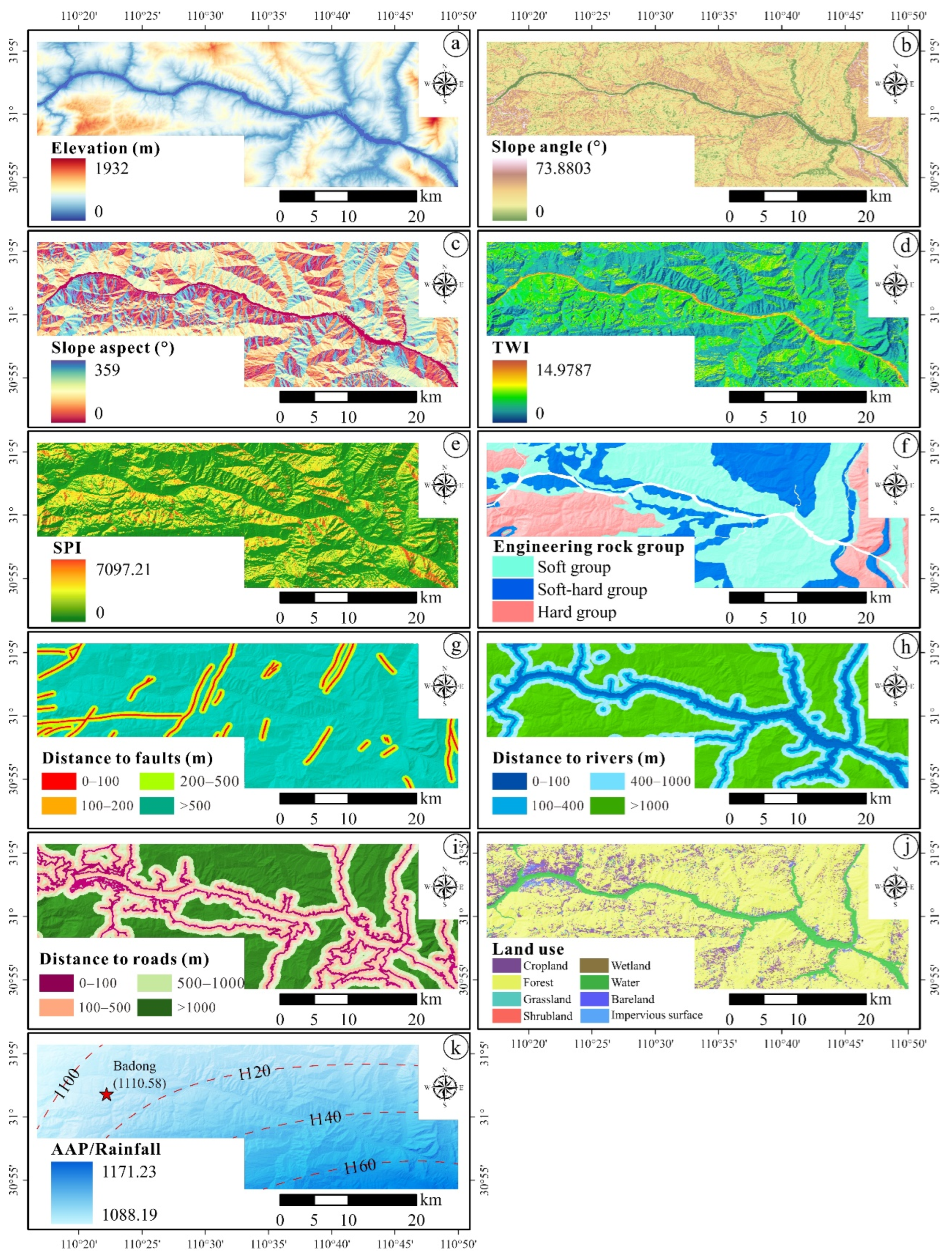
Per the above data sources, 11 influencing factors were extracted for LSM in the study area: elevation (EV), slope angle (SA), slope aspect (SAP), topographic wetness index (TWI), stream power index (SPI), engineering rock group (ERG), distance to faults (DF), distance to roads (DR), distance to rivers (DRV), land use (LU), and average annual precipitation (AAP). Topographic factors such as EV, SA, SAP, TWI, and SPI were acquired from the DEM with a 12.5 m resolution. Regarding the geological factors, ERG was generated by classifying lithologies into 3 classes, soft, soft–hard, and hard, based on their engineering characteristics [32]. Then, DF was calculated using Euclidean distance. Regarding the environmental and human activity factors, DRV and DRD were computed by Euclidean distance; LU was adopted from the FROM-GLS10 dataset with 10 m resolution, released by Tsinghua University; and AAP was determined from the precipitation data of 13 stations near the study area from 2015 to 2020, provided by the Hubei Provincial Bureau of Hydrology (http://113.57.190.228:8001) (accessed on 16 April 2022), using the inverse distance weighted (IDW) interpolation method.

2.2. Preparation of the Training and Test Datasets

According to previous studies, LSM was considered a binary classification task [38], where the mapping units were classified into two categories, landslides (value 1) and nonlandslides (value 0), and the probability distribution of landslide susceptibility ranged from 0 to 1. The choice of mapping units affects LSM; for this study, the most widely used grid cell with 12.5 m resolution was selected based on previous studies [39,40]. To evaluate landslide susceptibility, all 11 influencing factors and the landslide inventory map were converted into raster format with 12.5 m spatial resolution and aligned with the elevation raster, and the influencing factors are shown in Figure 4.
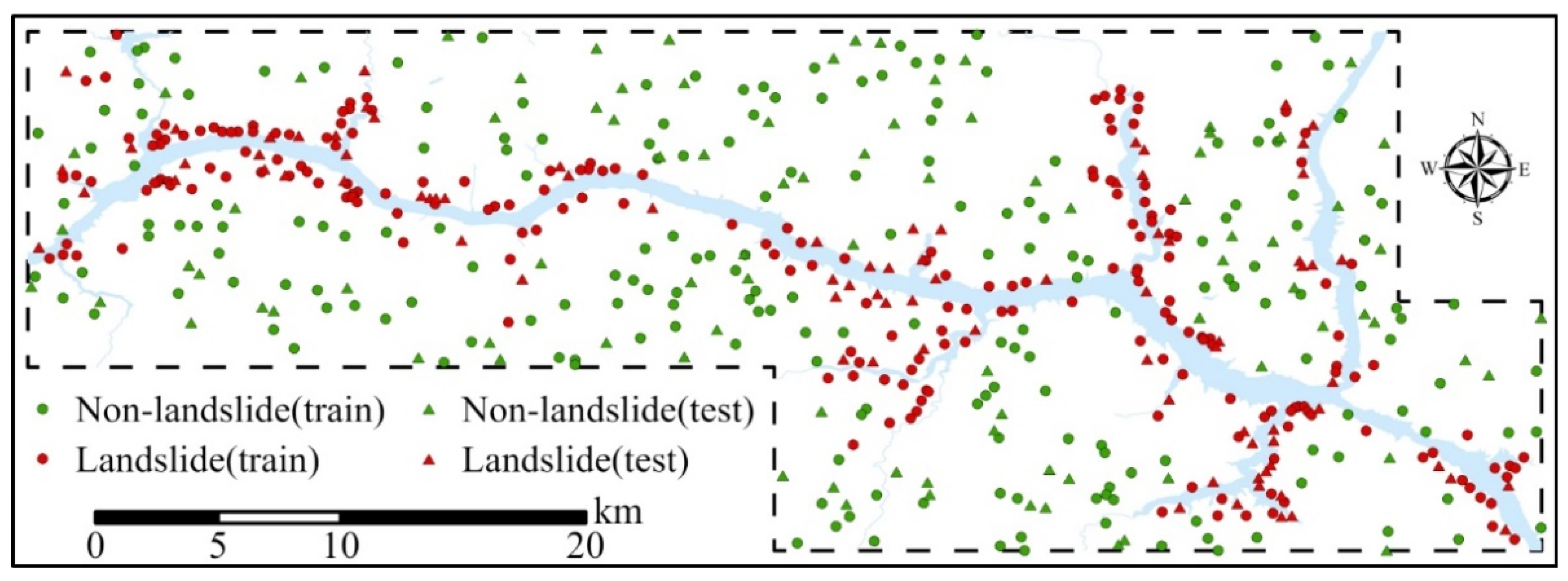
After conversion, a total of 290 landslide grid cells were acquired as the positive samples, and nonlandslide grid cells 50 m away from known landslides were randomly selected as negative samples at a ratio of 1:1 [41,42]. The total dataset with 580 samples was generated by merging the landslide grid cells (labeled as 1) and nonlandslide grid cells (labeled as 0). Since k-fold spatial cross-validation was chosen for model validation, the dataset was then divided randomly into training (70%, 204:202 landslide:nonlandslide samples) and testing (30%, 86:88 landslide:nonlandslide samples) datasets, as shown in Figure 5. Finally, the training and testing datasets were prepared with the corresponding values of the 11 landslide influencing factors [43].

2.3. Analysis of the Factors Influencing Landslides

Past studies have shown that multicollinearity, i.e., the nonindependence of influencing factors that may occur in a dataset, can lead to erroneous LSM [44]. Several methods have been proposed to quantify multicollinearity, such as Pearson’s correlation coefficient analysis [10,45,46], conditional analysis [47], and variance inflation factor (VIF) and tolerance (TOL) methods [5,48,49]. In this study, the most widely used methods, the VIF and TOL methods, were employed to identify multicollinearity among the influencing factors. VIF refers to the ratio of the variance between influencing factors in the presence of multicollinearity and in the absence of multicollinearity, and TOL is the inverse of VIF, which reflects the degree of increase in variance induced by multicollinearity. Generally, a VIF value greater than 5 or a TOL value less than 0.2 is considered to indicate strong multicollinearity between the influencing factors, which is regarded as unacceptable for analysis [18,24]. For Pearson’s correlation coefficient, values larger than 0.7 indicate high collinearity between influencing factors [50].

2.4. Landslide Susceptibility Models

In this study, a new LSM model named GCO-SVC was proposed, and six other popular models were selected for comparison: ANN, DT, KNN, RF, GRID-SVC, and GA-SVC models. All analyses were carried out using Python 3.6.9, scikit-learn 1.1.1, and ArcGIS Pro 2.9 in Windows 10 Pro 21H1 with an AMD Ryzen 7 5800H processor running at 3.2 GHz and 64 G RAM.

2.4.1. GCO-SVC

(1)
SVC
SVC is a popular classification algorithm based on Vapnik’s statistical learning theory, which minimizes a bound on a generalized risk based on the structural risk minimization principle [51,52,53]. SVC has been extensively applied to landslide susceptibility modeling, and its predictive ability has been demonstrated in numerous studies to be higher than that of other traditional methods [38,54]. However, the performance of an SVC model is heavily influenced by various hyperparameters, such as the penalty term ( C ), the kernel function, and its parameters.
min 1 2 | | w | | 2 + C i = 1   n ζ i
subject   to   y i [ ( w x i ) + b ] 1 ζ i ,   i = 1 , , n
where | | w | | is the normal constant of the hyperplane and b is a scalar basis.
For the penalty term ( C ), the larger the value is, the more severe is the penalty of the model for misclassification, but the model tends to be overfitted; the smaller the value is, the lighter is the penalty of the model for misclassification, but the model tends to be underfitted. Thus, a suitable penalty term ( C ) is crucial for an SVC model. The SVC kernels include linear, polynomial (poly), Gaussian (RBF), and sigmoid types; their formulas and kernel parameters are shown in Table 2. γ is the gamma term for all kernel types except linear, d is the polynomial degree term for the poly kernel, and r is the bias term in the poly and sigmoid kernels, which is usually ignored and set to the default value of 0 [55,56]. Among these four kernel functions, RBF usually provides better predictive performance in nonlinear classification for LSM than the other kernel functions [57,58]. Thus, in this study, the RBF kernel was employed for the SVC model to produce the LSM, and the hyperparameters for the RBF-SVC were the penalty term ( C ) and the gamma term ( γ ).
(2)
GCO
GCO is a new metaheuristic optimization algorithm proposed by Villaseñor; it is a novel multivariate continuous optimization algorithm inspired by the germinal center (GC) reaction [59]. The GCs, where B lymphocytes (B cells) and other immune cells are bounded by inactive B cells that form in the presence of an infection, can be divided into two zones: a dark zone, where clonal expansion occurs and somatic cells are located, and a light zone, where competition for Ag internalization and helper T-cell binding occurs [60]. In this study, GCO was employed to search for the optimal hyperparameters (C and gamma) for the RBF-SVC model, which comprised 4 steps, initialization, dark-zone processing, light-zone processing, and postprocessing, as shown in the flowchart in Figure 6.
Step 1: Initialization. A population of B cells with a total number N is initialized, and every B cell B i stores a candidate solution that is randomly initialized in the hyperparameter space. Additionally, each B cell has a cell counter B i c with an initial value of 0 and a life signal B i ε with an initial value of 70, which means that the cell has a 70% chance of duplication and a 30% chance of death. Importantly, B i C and B i ε will change and influence the evolution throughout the life of GCO.
Step 2: Dark-zone processing. The dark-zone process is the first part of each iteration, which is responsible for the life management and mutation of B cells. First, for each B cell B i , a random number with a uniform range from 0 to 100 is generated and compared with the life signal B i ε to decide the destiny of the B cell: duplication or death. Duplication means adding one to B i c , while death is the reverse. Then, a mutated B cell is generated by mutation, which is performed using modified differential evolution (DE)-like mutation process. The key parameters of the mutation are c r and w f ; the first parameter controls the difficulty of mutation and ranges from 0 to 1, and the second parameter is the coefficient of mutation. The global best solution of each iteration is recorded during the mutation.
Step 3: Light-zone processing. The light-zone process is the second part of each iteration after the mutation of each B cell, which manages the fitness calculation, aging, and reward of each B cell. First, each B cell is aged by resetting its life signal to 10. Second, for each B cell B i , the parameters C and gamma inside it are used for the construction of the RBF-SVC model, and the fitness of B i is calculated using 5-fold cross-validation on the training set. Then, the f i t i of each B cell is obtained based on Equation (3). Third, each B cell is rewarded by adding 10 f i t i to its life signal B i ε .
f i t i = { f ( B i ) max f ( B k ) min f ( B k ) max f ( B k )       for   minimum min f ( B k ) f ( B i ) min f ( B k ) max f ( B k )     for   maximum
Step 4: Postprocessing. Steps 2 and 3 are looped until the end of all iterations to obtain the optimum hyperparameters ( C and γ ) of the RBF-SVC model by decoding the global best solution.
(3)
Implementation of the GCO-SVC model
The hyperparameter space of RBF-SVC includes C and γ , both of which range from 10 3 to 10 4 . The optimum hyperparameters were obtained using the above GCO algorithm, and then the SVC model for LSM was constructed with the best C and γ and trained using the training set acquired in Section 2.2. Thus, the whole process described above was named GCO-SVC to complete the LSM of the study area, and the hyperparameter search space of the GCO-SVC model is listed in Table 3.

2.4.2. Models for Comparison

For a comparison study, six popular models for LSM, ANN [6,7], DT [12,13], KNN [15,16], RF [10,11], GRID-SVC [10,58], and GA-SVC [25], were selected in this study. The base versions of the above models require hyperparameter optimization, where ANN, DT, KNN, RF, and GRID-SVC use grid search coupled with 5-fold cross-validation, and GA-SVC uses a GA combined with 5-fold cross-validation. Since these models are very mature and widely validated, their principles are described only briefly here, and the hyperparametric optimization space of each model is shown in Table 3.
(1)
ANN
The ANN model is a widely used model for LSM and has great nonlinear mapping capability and strong generalization ability [61]. An ANN generally consists of an input layer, an output layer, and one or more hidden layers, and each layer contains several neurons, which are the basic units of the model. The nodes of the input layer correspond to the landslide influencing factors in turn, and the nodes in the output layer respond to the probability of landslide susceptibility. The hidden layers are the bridge between the input and output layers and typically contain one or multiple layers. Based on previous studies, an ANN containing an input layer, an output layer, and a hidden layer was constructed for comparison in this study, and its hyperparameter space focused on the number of hidden layers and the L2 penalty parameter α . The other parameters were set as the default values: “relu” as the activation function, stochastic gradient-based optimizer as the solver, 500 as maximum iterations, and 10 4 as the tolerance of the optimization.
(2)
DT
The DT model is a nonparametric supervised deep learning model and has been applied successfully for LSM [12,62,63]. It is built to find a set of decision rules to predict landslide susceptibility according to landslide influencing factors. Various DT algorithms have been developed, such as ID3 [64], C4.5 [65], C5.0 [66], and CART [67,68]. CART builds binary trees with features and thresholds that yield maximum information gain at each node; CART was selected for the comparison study. The main hyperparameters for the DT model are the maximum depth of the decision tree and the minimum number of samples, and the search space is listed in Table 3.
(3)
KNN
The KNN algorithm is a traditional nonparametric supervised statistics method that was proposed in the 1960s [69]. The principle of KNN is simplicity: a sample belongs to the category if the majority of the K most similar or most neighboring samples in the feature space fall into that category as well. Due to the simplicity and intuitiveness of the principle and its good performance, it has been widely used in various classification studies, including LSM [10,15,70]. Regarding the hyperparameters of KNN, “N neighbors” is the number of neighbors to use by default for k-neighbor queries; weight functions are used in prediction, including “uniform”, in which all neighborhoods are weighed equally, and “distance”, in which weight points are given by the inverse of their distance; the “distance function” includes two types: M a n h a t t a n and E u c l i d e a n distance.
(4)
RF
RF is a meta-estimator that resumes multiple independent decision trees at different sample sizes by random sampling and uses averaging to combine multiple decision trees for classification to improve prediction accuracy and control overfitting [11,71]. The RF model is simple to implement and is faster to train and less prone to overfitting than other models, and it can date the impact between each feature [10,72]. For the construction of the RF model, “Number of estimators” is the total number of decision trees, and “Criterion” is the function used to measure the quality of a split.
(5)
GRID-SVC
To perform a comprehensive analysis, a grid search with the 5-fold cross-validation method is applied to the SVC hyperparameter search, and the model is labeled GRID-SVC. This model uses the same core SVC model and hyperparametric search space as the GCO-SVC model, differing only in the search method.
(6)
GA-SVC
The GA is a computational model of biological evolution that simulates the natural selection and genetic mechanism of Darwinian evolution and is used to search for the optimal solution by simulating a natural evolutionary process [25,73]. GA has been heavily applied to hyperparameter optimization for SVC in past studies, and it is a metaheuristic algorithm like GCO. Thus, the GA is employed to optimize the hyperparameters of the SVC model in the same search space as the GCO-SVC model, and the model is named GA-SVC.

2.5. Model Evaluation Criteria

The LSM problem is generally considered a binary classification problem that is positive for landslide units and negative for nonlandslide units, and the probability that the unit is positive is considered its susceptibility, which ranges from 0 to 1. Four metrics were utilized for model evaluation: accuracy, F1 score, Log loss, and AUC. Accuracy represents the classification accuracy of a model and is given by:
Accuracy = T P + T N T P + T N + F P + F N
where TP is the true-positive prediction, TN is the true-negative prediction, FP is the false-positive prediction, and FN is the false-negative prediction.
The F1 score is another widely used accuracy metric; it is considered a harmonic mean of model accuracy and recall and is given by:
F 1   score = 2 T P 2 T P + F P + F N
Logarithmic loss (Log loss) represents the closeness of the predicted probability to the corresponding true value. The larger the deviation of the predicted probability from the true value, the higher the Log loss. The Log loss can be calculated using:
Log   loss = 1 N i = 1 N y i log ( p ( y i = 1 ) ) + ( 1 y i ) p ( y i = 0 )
where N is the total number of samples, y i is the true label of the i th sample, p ( y i = 0 ) is the probability of the predicted label of the i th sample being 0, and p ( y i = 1 ) is the probability of the predicted label of the i th sample being 1.
The receiver operating characteristic (ROC) curve is a graph showing the performance of a classification model at all classification thresholds. It is plotted by the true-positive rate (TPR, given by T P / ( T P + F N ) ) against the false-positive rate (FPR, given by F P / ( T N + F P ) ) at different thresholds. Then, the area under the ROC curve (AUC) can be calculated, which provides a comprehensive evaluation of performance for all probability classification thresholds.
To assess the statistical significance of systematic pairwise differences among the seven landslide models, the Wilcoxon signed-rank test was employed. Its results contain two values, p and z , that describe the difference between the models. For a pair of models, if p is below the 0.05 significance level and z exceeds the critical range (−1.96 to +1.96), their performance can be considered different [38,43].
Finally, to evaluate the contributions of different landslide influencing factors to the models, permutation feature importance (PFI) was calculated, which is defined as the reduction of the model score when a single feature value is randomly shuffled [74]. The importance of the influencing factor is obtained by averaging the reduction of the model output scores that are calculated by shuffling the influencing factor N times. In this study, Log loss was selected as the score function of the models for calculating the PFI, and the number of times a feature is randomly shuffled was set at 30.

3. Results

3.1. Influencing Factor Analysis

VIF analysis was employed for the multicollinearity analysis of the landslide influencing factors, and the results are shown in Table 4. The influencing factor with the largest VIF value, 2.976, was DRV, and that with the smallest value, 1.104, was DF. None of the influencing factors had a VIF value greater than 5 or a TOL smaller than 0.2, indicating a lack of significant multicollinearity [18,75]. Thus, all the landslide influencing factors were taken into account for LSM.

3.2. Optimal Hyperparameters

In this study, all seven models were optimized using grid search or metaheuristic algorithms with hyperparameter search spaces (listed in Table 3), as described in Section 2.4. The optimum hyperparameters and the corresponding best score obtained after the optimization of the seven models are listed in Table 5, together with other parameter settings of each model. The results show that the GCO-SVC model achieved the best score (0.231471), followed by the GA-SVC (0.232593), RF (0.238102), GRID-SVC (0.243250), KNN (0.290551), DT (0.324234), and ANN (0.434876) models. Comparison of the grid search optimized models (ANN, DT, KNN, and GRID-SVC) with the metaheuristic algorithm optimized models (GA-SVC and GCO-SVC) revealed that the best scores of the latter models were less than 0.235, while those of the former models were greater than 0.235. Thus, the models optimized by the metaheuristic algorithms performed better than the models optimized by the grid search algorithm.

3.3. Model Performance Comparison

The optimal hyperparameters and training set were applied for model construction and training, and the testing set with 174 samples was used for model evaluation. Then, the performance metrics of the seven models on the training and testing sets were acquired. Table 6 lists the accuracy, F1 score, Log loss, and AUC values of the seven models on the training and testing sets. The GCO-SVC model achieved the best scores of all four metrics: an accuracy of 0.9425, an F1 score of 0.9412, a Log loss of 1.9850, and an AUC of 0.9425. The performance of GCO-SVC was consistent between the training and testing sets, which indicates that the model has a strong generalization ability without overfitting or underfitting. The other two SVC-based models, GA-SVC (AUC = 0.9371) and GRID-SVC (AUC = 0.9198), followed in second and third place, respectively, with slightly lower performance and good generalization. The performance of ANN, KNN, and RF on the training set was perfect, each yielding an accuracy of 1, an F1 score of 1, a Log loss of 0, and an AUC of 1, but they did not achieve corresponding performance on the testing set (accuracy, F1 score, and AUC less than 0.91 and Log loss > 3.1), which revealed overfitting. The DT model exhibited the poorest performance among the models on both the training set and the testing set, with the poorest scores for all metrics. Its performance was consistent between the two sets, which demonstrated the absence of overfitting or underfitting by DT. The ROC curves of the seven models based on the testing set are shown in Figure 7a.
To evaluate the convergence of the GCO-SVC model, the same metaheuristic-based GA-SVC model was employed for the comparison of the convergence curves, as shown in Figure 7b. As evident from Table 5, GCO-SVC and GA-SVC have almost the same parameter settings for hyperparameter optimization, including the parameters of the optimization algorithm (epoch, population) and the default parameters of SVC (such as tolerance and max iterations), and they have the same hyperparameter search space. The convergence curves in Figure 7b show that compared to GA-SVC, GCO-SVC converged faster initially and slower in the middle, but it continued to converge throughout the process, finally obtaining a lower loss than GA-SVC at the end of the iteration. In summary, GCO-SVC offered better performance than GA-SVC and powerful continuous optimization but may require many iterations.
In the pairwise model comparison, GCO-SVC was compared with the other six models using the Wilcoxon signed-rank test, and the results are shown in Table 7. The performance of the GCO-SVC model was significantly different from that of the other six models, with all the p values being lower than 0.05 and all z values exceeding the critical range (−1.96 to +1.96).

3.4. Landslide Susceptibility Maps

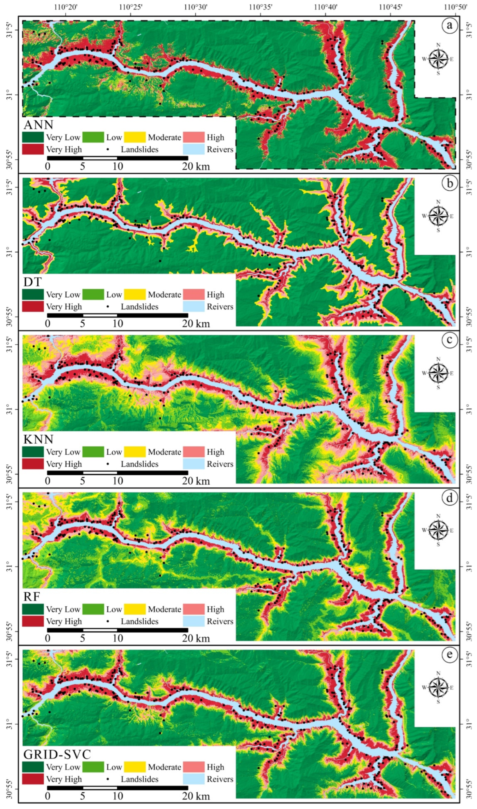
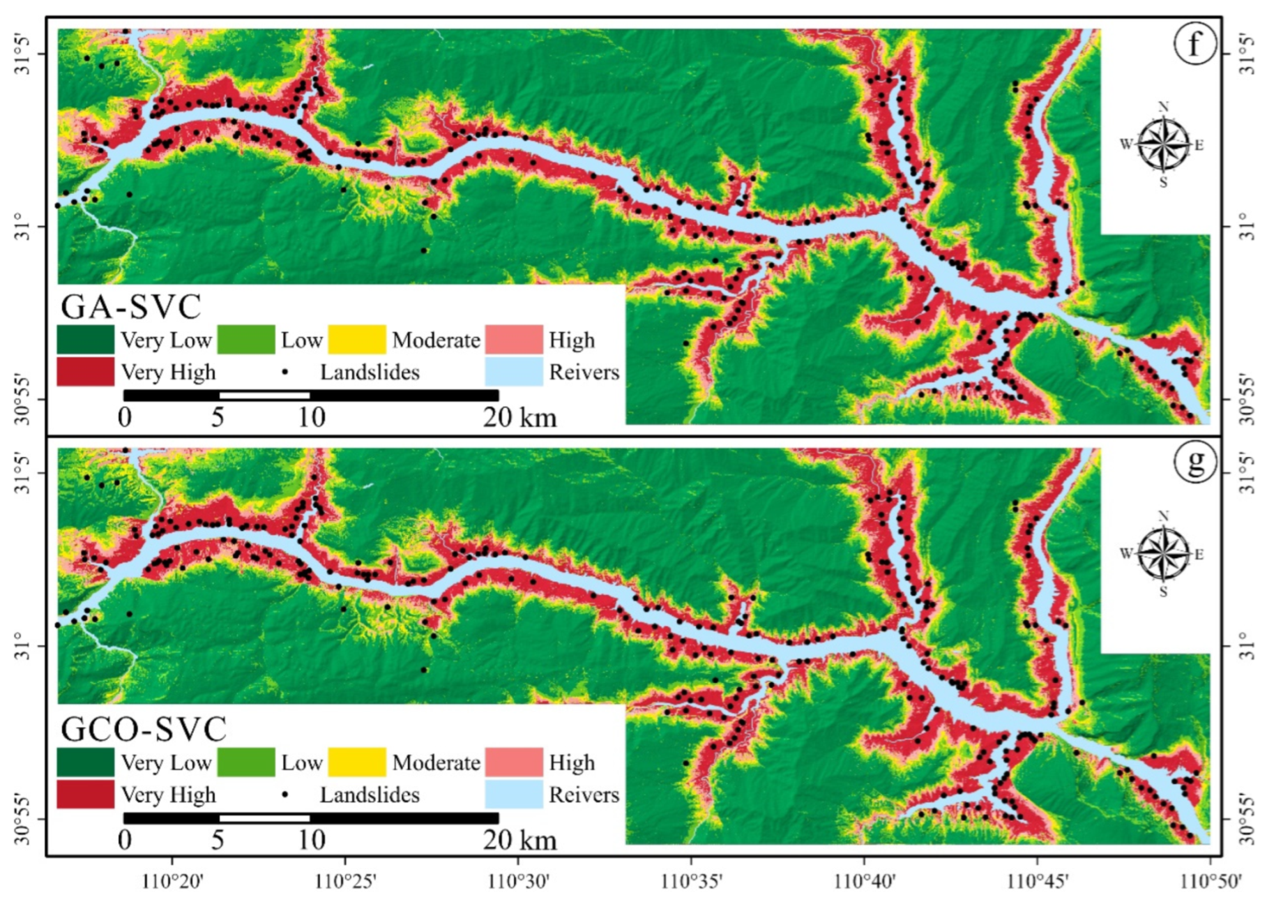
Seven trained models using the optimal hyperparameters and training set were constructed to predict the landslide susceptibility indices for all the mapping units in the study area. Then, all the mapping units were divided into five susceptibility levels: very low (0.0 to 0.1), low (0.1 to 0.3), moderate (0.3 to 0.5), high (0.5 to 0.8), and very high (0.8 to 1.0). Finally, seven landslide susceptibility maps were produced from the ANN, DT, KNN, RF, GRID-SVC, GA-SVC, and GCO-SVC models, as shown in Figure 8, and the statistical analysis results for the landslide distribution at different susceptibility levels are listed in Table 8.
Table 8 shows that the very high and high susceptibility levels accounted for 16.40%, 15.59%, 22.86%, 13.81%, 16.50%, 16.54%, and 16.38%; the moderate levels accounted for 1.94%, 5.72%, 10.25%, 6.85%, 4.53%, 4.17%, and 4.04%; and the very low and low susceptibility levels accounted for 81.66%, 78.69%, 66.89%, 79.35%, 78.98%, 79.29%, and 79.58% of the total area for ANN, DT, KNN, RF, GRID-SVC, GA-SVC and GCO-SVC, respectively. KNN obtained the highest percentage of very high- and high-susceptibility units to total landslides (92.79%), followed by GCO-SVC (86.76%), GA-SVC (86.72%), GRID-SVC (86.24%), ANN (84.98%), RF (80.47%), and DT (75.60%).
Figure 8c and the above results show that the LSM produced by KNN generally reflected higher susceptibility and differed significantly from the LSM obtained with the other six models; thus, it is not recommended. The results of ANN showed that very low- and very high-sensitivity units accounted for 91.68% of the total area, with the former accounting for 78.19% and the latter for 13.49%; these values highly differ. DT showed similar performance to ANN, having an even higher very low-susceptibility percentage of 78.69%; thus, neither model showed good generalization. Figure 8d shows that RF achieved a better result than ANN, DT, and KNN in terms of susceptibility distribution, but the proportion of very high or high susceptibility levels was significantly lower than that of the other models, indicating that its results were conservative. In addition, the LSM produced by DT had an intermediate break and no units classified into the low susceptibility level, as shown in both Table 8 and Figure 8b. The SVC-based models GRID-SVC, GA-SVC, and GCO-SVC produced similar landslide susceptibility maps but differed in many details. For example, the proposed GCO-SVC model obtained the best performance with respect to the percentage of very high-susceptibility units to total landslides (74.78%), followed by GA-SVC (74.57%) and GRID-SVR (73.09%), and the numbers of pixels classified into very high-susceptibility units based on GCO-SVC exceeded the corresponding numbers obtained via GA-SVC and GRID-SVC by 141,495 and 8708, respectively.

4. Discussion

4.1. PFI of the Influencing Factors

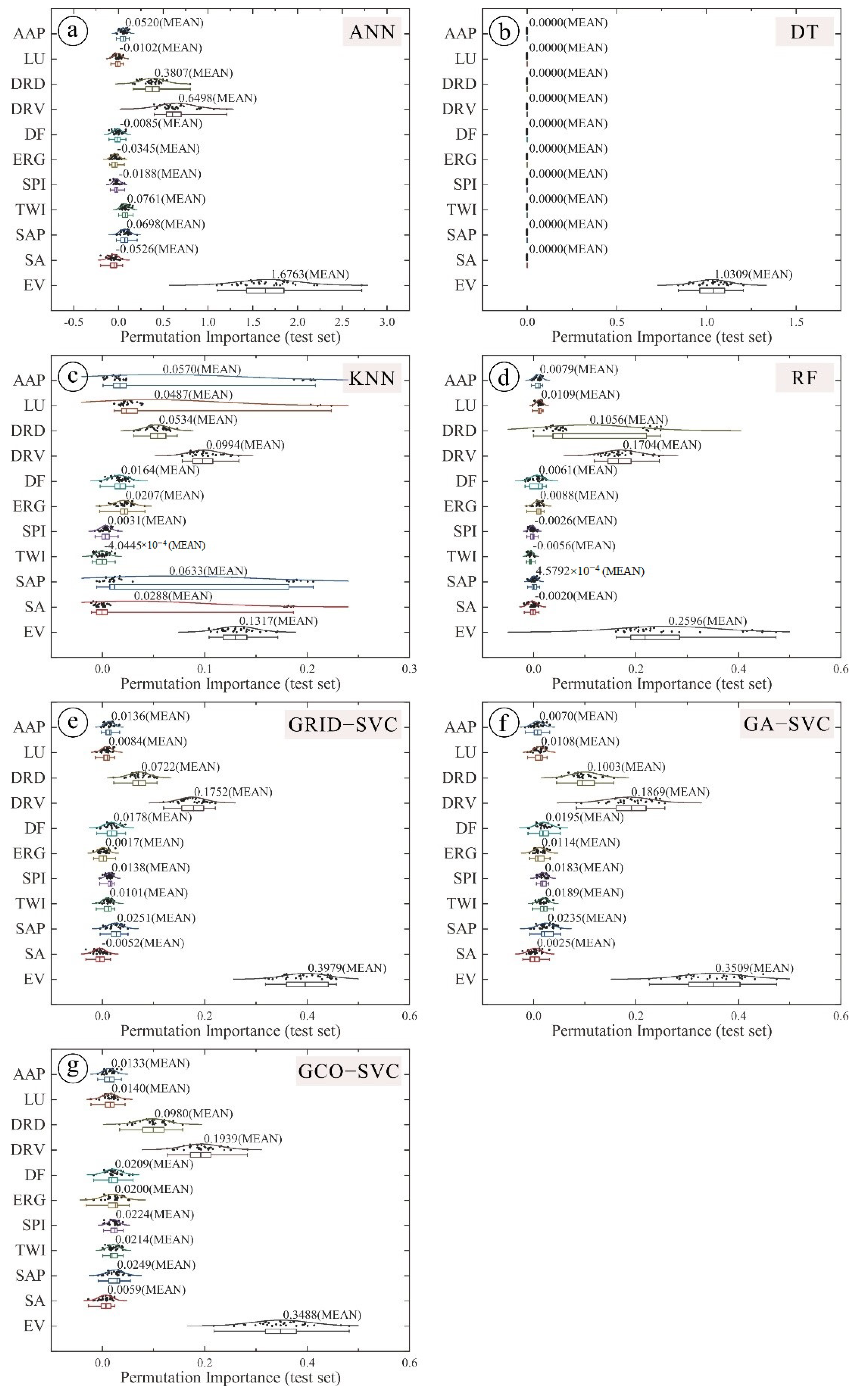
To assess the predictive power of the influencing factors, PFI was employed to determine the contributions of the different influencing factors to the predictions of the seven models, as described in Section 2.5. The PFI score of each influencing factor is shown in Figure 9. The results show that EV, DRV, and DRD were the most sensitive influencing factors affecting the landslide susceptibility predicted by ANN, RF, GRID-SVC, GA-SVC, and GCO-SVC. For GCO-SVC, the PFI of each factor was stable, and EV was the most sensitive factor, followed by DRV, DRD, SAP, SPI, TWI, DF, ERG, LU, APP, and SA. For DT, only EV affected the results, which is inconsistent with reality; thus, the model is not recommended. For KNN, the variance of the PFI of each factor was large, but the mean values were generally consistent with those of the other models. In conclusion, EV, DRV, and DRD were the top three landslide influencing factors in the study area.

4.2. Sensitivity Analysis of the Parameters of the GCO-SVC Model

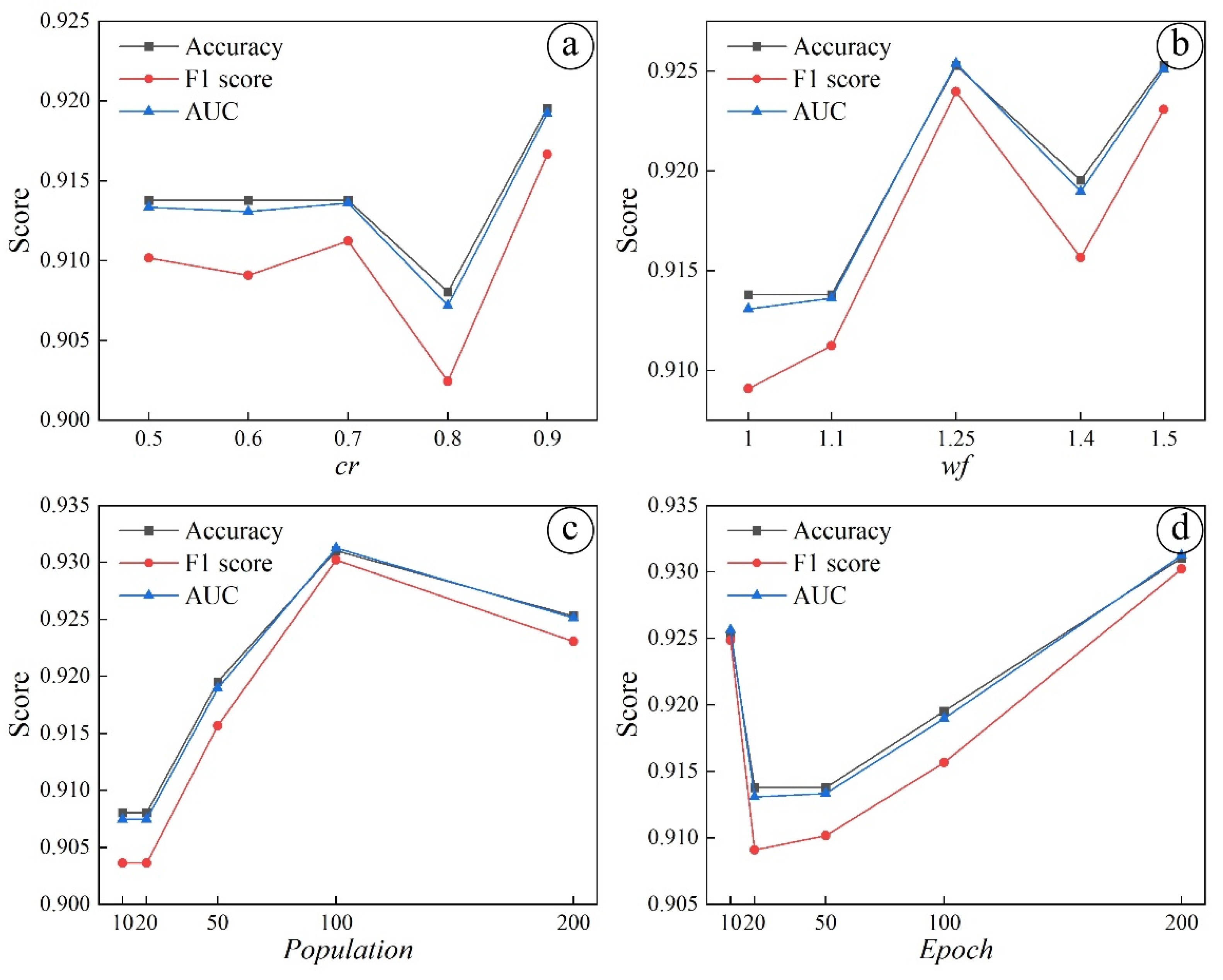
According to the principle of the GCO metaheuristic optimization algorithm described in Section 2.4.1, the model has four important parameters that affect the performance of the algorithm: c r , w f , P o p u l a t i o n , and E p o c h , which represent the difficulty of mutation, the coefficient of mutation, the total population, and the number of iterations, respectively. The set of default parameters, c r = 0.7 ,   w f = 1.25 ,   P o p u l a t i o n = 100 , and E p o c h = 100 , was taken as the benchmark, and the control variable method was used to vary the other parameters and observe the performance of the model on the validation set to determine the effect of each parameter on the GCO-SVC model. Figure 10 shows the performance of the GCO-SVC model under different combinations of hyperparameters.
Figure 10a shows that an increase in the difficulty of mutation ( c r ) does not significantly improve the performance of the model and can even have the opposite effect (e.g., when c r = 0.8); thus, it is recommended that c r be set to 0.7. The performance of the model under different values of the coefficient of mutation ( w f ) and the total population ( P o p u l a t i o n ) in Figure 10 exhibits a mountain shape, with the model performing optimally when w f = 1.25 and P o p u l a t i o n = 100 . In regard to the number of iterations ( E p o c h ), an increase in E p o c h improves the performance of the proposed GCO-SVC model, but a large increase in epochs may lead to overfitting and consume a considerable amount of computing capacity and time; thus, it is recommended that E p o c h be set at 200. In conclusion, the suggested combination of hyperparameters for the GCO-SVC model is c r = 0.7 ,     w f = 1.25 ,     P o p u l a t i o n = 100 , and E p o c h = 200 .

5. Conclusions

In this study, a new model called GCO-SVC was proposed for assessing landslide susceptibility in the Zigui to Badong basins of the TGRA. The proposed GCO-SVC model was validated for landslide susceptibility in the study area through the analysis of 11 influencing factors. Six commonly used models, ANN, DT, KNN, RF, GRID-SVC, and GA-SVC, were used for comparative analysis based on the objective measures of accuracy, F1 score, Log loss, and AUC. In addition, the PFI scores of all influencing factors and the sensitivities of the parameters of the GCO-SVC model were evaluated. The following conclusions were drawn from the comparison study: (1) The proposed GCO-SVC model demonstrated good fitting and generalization in the evaluation of landslide susceptibility in the study area. (2) The proposed GCO-SVC model obtained optimal results across all metrics, i.e., AUC, accuracy, F1 score, and Log loss, and performed significantly better than the other six models. (3) EV, DRV, and DRD were found to be the top three most influential factors in this study area by PFI analysis. (4) The optimal combination of parameters for the proposed GCO-VC model was identified through parameter sensitivity analysis, which showed that the performance of GCO-SVC can be improved by appropriately increasing the number of epochs. In summary, the GCO-SVC model holds promise for landslide susceptibility analysis and performed better than six other popular models in the study area. In the future, the proposed GCO-SVC model should be applied to additional cases to validate its adaptability.

Author Contributions

Conceptualization, D.X. and H.T.; data curation, D.X., S.S. and C.T.; funding acquisition, H.T.; methodology, D.X.; project administration, H.T.; resources, H.T.; software, D.X.; supervision, H.T.; validation, H.T., S.S. and C.T.; visualization, S.S., C.T. and B.Z.; writing—original draft, D.X.; writing—review and editing, D.X., H.T., S.S., C.T. and B.Z. All authors have read and agreed to the published version of the manuscript.

Funding

This research was supported by the Major Program of the National Natural Science Foundation of China (No. 42090055), the National Major Scientific Instruments and Equipment Development Projects of China (No. 41827808), and the State Scholarship Fund from the China Scholarship Council (No. 202106410076).

Data Availability Statement

The data and materials that support the findings of this study are available from the first author and the corresponding author, Ding Xia and Huiming Tang, upon reasonable request.

Conflicts of Interest

The authors declare that they have no conflict of interest.

References

  1. Tang, H.; Wasowski, J.; Juang, C.H. Geohazards in the three Gorges Reservoir Area, China—Lessons learned from decades of research. Eng. Geol. 2019, 261, 105267. [Google Scholar] [CrossRef]
  2. Haque, U.; da Silva, P.F.; Devoli, G.; Pilz, J.; Zhao, B.; Khaloua, A.; Wilopo, W.; Andersen, P.; Lu, P.; Lee, J.; et al. The human cost of global warming: Deadly landslides and their triggers (1995–2014). Sci. Total Environ. 2019, 682, 673–684. [Google Scholar] [CrossRef]
  3. Zêzere, J.L.; Ferreira, A.B.; Rodrigues, M.L. Landslides in the North of Lisbon Region (Portugal): Conditioning and triggering factors. Phys. Chem. Earth Part A Solid Earth Geod. 1999, 24, 925–934. [Google Scholar] [CrossRef]
  4. Jebur, M.N.; Pradhan, B.; Tehrany, M.S. Optimization of landslide conditioning factors using very high-resolution airborne laser scanning (LiDAR) data at catchment scale. Remote Sens. Environ. 2014, 152, 150–165. [Google Scholar] [CrossRef]
  5. Wang, Y.; Fang, Z.; Hong, H. Comparison of convolutional neural networks for landslide susceptibility mapping in Yanshan County, China. Sci. Total Environ. 2019, 666, 975–993. [Google Scholar] [CrossRef] [PubMed]
  6. Sezer, E.A.; Pradhan, B.; Gokceoglu, C. Manifestation of an adaptive neuro-fuzzy model on landslide susceptibility mapping: Klang valley, Malaysia. Expert Syst. Appl. 2011, 38, 8208–8219. [Google Scholar] [CrossRef]
  7. Kalantar, B.; Pradhan, B.; Naghibi, S.A.; Motevalli, A.; Mansor, S. Assessment of the effects of training data selection on the landslide susceptibility mapping: A comparison between support vector machine (SVM), logistic regression (LR) and artificial neural networks (ANN). Geomat. Nat. Hazards Risk 2017, 9, 49–69. [Google Scholar] [CrossRef]
  8. Choi, J.; Oh, H.-J.; Lee, H.-J.; Lee, C.; Lee, S. Combining landslide susceptibility maps obtained from frequency ratio, logistic regression, and artificial neural network models using ASTER images and GIS. Eng. Geol. 2012, 124, 12–23. [Google Scholar] [CrossRef]
  9. Wang, H.B.; Li, J.M.; Zhou, B.; Zhou, Y.; Yuan, Z.Q.; Chen, Y.P. Application of a hybrid model of neural networks and genetic algorithms to evaluate landslide susceptibility. Geoenviron. Disasters 2017, 4, 15. [Google Scholar] [CrossRef] [Green Version]
  10. Adnan, M.S.G.; Rahman, M.S.; Ahmed, N.; Ahmed, B.; Rabbi, M.F.; Rahman, R.M. Improving Spatial Agreement in Machine Learning-Based Landslide Susceptibility Mapping. Remote Sens. 2020, 12, 3347. [Google Scholar] [CrossRef]
  11. Zhou, X.; Wen, H.; Zhang, Y.; Xu, J.; Zhang, W. Landslide susceptibility mapping using hybrid random forest with GeoDetector and RFE for factor optimization. Geosci. Front. 2021, 12, 101211. [Google Scholar] [CrossRef]
  12. Sameen, M.I.; Pradhan, B.; Bui, D.T.; Alamri, A.M. Systematic sample subdividing strategy for training landslide susceptibility models. CATENA 2020, 187, 104358. [Google Scholar] [CrossRef]
  13. Marjanović, M.; Kovačević, M.; Bajat, B.; Voženílek, V. Landslide susceptibility assessment using SVM machine learning algorithm. Eng. Geol. 2011, 123, 225–234. [Google Scholar] [CrossRef]
  14. Yalcin, A.; Reis, S.; Aydinoglu, A.C.; Yomralioglu, T. A GIS-based comparative study of frequency ratio, analytical hierarchy process, bivariate statistics and logistics regression methods for landslide susceptibility mapping in Trabzon, NE Turkey. CATENA 2011, 85, 274–287. [Google Scholar] [CrossRef]
  15. Avand, M.; Janizadeh, S.; Naghibi, S.A.; Pourghasemi, H.R.; Khosrobeigi Bozchaloei, S.; Blaschke, T. A Comparative Assessment of Random Forest and k-Nearest Neighbor Classifiers for Gully Erosion Susceptibility Mapping. Water 2019, 11, 2076. [Google Scholar] [CrossRef] [Green Version]
  16. Rabby, Y.W.; Hossain, M.B.; Abedin, J. Landslide susceptibility mapping in three Upazilas of Rangamati hill district Bangladesh: Application and comparison of GIS-based machine learning methods. Geocarto Int. 2021. [Google Scholar] [CrossRef]
  17. Huang, F.; Yin, K.; Huang, J.; Gui, L.; Wang, P. Landslide susceptibility mapping based on self-organizing-map network and extreme learning machine. Eng. Geol. 2017, 223, 11–22. [Google Scholar] [CrossRef]
  18. Zhou, C.; Yin, K.; Cao, Y.; Ahmed, B.; Li, Y.; Catani, F.; Pourghasemi, H.R. Landslide susceptibility modeling applying machine learning methods: A case study from Longju in the Three Gorges Reservoir area, China. Comput. Geosci. 2018, 112, 23–37. [Google Scholar] [CrossRef] [Green Version]
  19. Hong, H.; Liu, J.; Zhu, A.X. Modeling landslide susceptibility using LogitBoost alternating decision trees and forest by penalizing attributes with the bagging ensemble. Sci. Total Environ. 2020, 718, 137231. [Google Scholar] [CrossRef] [PubMed]
  20. Sun, D.; Xu, J.; Wen, H.; Wang, D. Assessment of landslide susceptibility mapping based on Bayesian hyperparameter optimization: A comparison between logistic regression and random forest. Eng. Geol. 2021, 281, 105972. [Google Scholar] [CrossRef]
  21. Sun, D.; Wen, H.; Wang, D.; Xu, J. A random forest model of landslide susceptibility mapping based on hyperparameter optimization using Bayes algorithm. Geomorphology 2020, 362, 107201. [Google Scholar] [CrossRef]
  22. Ma, J.; Wang, Y.; Niu, X.; Jiang, S.; Liu, Z. A comparative study of mutual information-based input variable selection strategies for the displacement prediction of seepage-driven landslides using optimized support vector regression. Stoch. Environ. Res. Risk Assess. 2022. [Google Scholar] [CrossRef]
  23. Zhang, J.; Tang, H.; Tannant, D.D.; Lin, C.; Xia, D.; Liu, X.; Zhang, Y.; Ma, J. Combined forecasting model with CEEMD-LCSS reconstruction and the ABC-SVR method for landslide displacement prediction. J. Clean. Prod. 2021, 293, 126205. [Google Scholar] [CrossRef]
  24. Merghadi, A.; Yunus, A.P.; Dou, J.; Whiteley, J.; ThaiPham, B.; Bui, D.T.; Avtar, R.; Abderrahmane, B. Machine learning methods for landslide susceptibility studies: A comparative overview of algorithm performance. Earth-Sci. Rev. 2020, 207, 103225. [Google Scholar] [CrossRef]
  25. Niu, R.; Wu, X.; Yao, D.; Peng, L.; Ai, L.; Peng, J. Susceptibility Assessment of Landslides Triggered by the Lushan Earthquake, April 20, 2013, China. IEEE J. Sel. Top. Appl. Earth Obs. Remote Sens. 2014, 7, 3979–3992. [Google Scholar] [CrossRef]
  26. Chen, Y.-R.; Chen, J.-W.; Hsieh, S.-C.; Ni, P.-N. The Application of Remote Sensing Technology to the Interpretation of Land Use for Rainfall-Induced Landslides Based on Genetic Algorithms and Artificial Neural Networks. IEEE J. Sel. Top. Appl. Earth Obs. Remote Sens. 2009, 2, 87–95. [Google Scholar] [CrossRef]
  27. Moayedi, H.; Mehrabi, M.; Mosallanezhad, M.; Rashid, A.S.A.; Pradhan, B. Modification of landslide susceptibility mapping using optimized PSO-ANN technique. Eng. Comput. 2019, 35, 967–984. [Google Scholar] [CrossRef]
  28. Wang, J.; Su, A.; Xiang, W.; Yeh, H.-F.; Xiong, C.; Zou, Z.; Zhong, C.; Liu, Q. New data and interpretations of the shallow and deep deformation of Huangtupo No. 1 riverside sliding mass during seasonal rainfall and water level fluctuation. Landslides 2016, 13, 795–804. [Google Scholar] [CrossRef]
  29. Su, X.; Tang, H.; Huang, L.; Shen, P.; Xia, D. The role of pH in red-stratum mudstone disintegration in the Three Gorges reservoir area, China, and the associated micromechanisms. Eng. Geol. 2020, 279, 105873. [Google Scholar] [CrossRef]
  30. Hungr, O.; Fell, R.; Couture, R.; Eberhardt, E. Landslide Risk Management; CRC Press: Boca Raton, FL, USA, 2005. [Google Scholar]
  31. Tang, M.; Xu, Q.; Yang, H.; Li, S.; Iqbal, J.; Fu, X.; Huang, X.; Cheng, W. Activity law and hydraulics mechanism of landslides with different sliding surface and permeability in the Three Gorges Reservoir Area, China. Eng. Geol. 2019, 260, 105212. [Google Scholar] [CrossRef]
  32. Hua, Y.; Wang, X.; Li, Y.; Xu, P.; Xia, W. Dynamic development of landslide susceptibility based on slope unit and deep neural networks. Landslides 2020, 18, 281–302. [Google Scholar] [CrossRef]
  33. Hu, X.; Huang, C.; Mei, H.; Zhang, H. Landslide susceptibility mapping using an ensemble model of Bagging scheme and random subspace–based naïve Bayes tree in Zigui County of the Three Gorges Reservoir Area, China. Bull. Eng. Geol. Environ. 2021, 80, 5315–5329. [Google Scholar] [CrossRef]
  34. Petschko, H.; Brenning, A.; Bell, R.; Goetz, J.; Glade, T. Assessing the quality of landslide susceptibility maps—Case study Lower Austria. Nat. Hazards Earth Syst. Sci. 2014, 14, 95–118. [Google Scholar] [CrossRef] [Green Version]
  35. Goetz, J.N.; Brenning, A.; Petschko, H.; Leopold, P. Evaluating machine learning and statistical prediction techniques for landslide susceptibility modeling. Comput. Geosci. 2015, 81, 1–11. [Google Scholar] [CrossRef]
  36. Chen, T.; Niu, R.; Du, B.; Wang, Y. Landslide spatial susceptibility mapping by using GIS and remote sensing techniques: A case study in Zigui County, the Three Georges reservoir, China. Environ. Earth Sci. 2015, 73, 5571–5583. [Google Scholar] [CrossRef]
  37. Gong, P.; Liu, H.; Zhang, M.; Li, C.; Wang, J.; Huang, H.; Clinton, N.; Ji, L.; Li, W.; Bai, Y.; et al. Stable classification with limited sample: Transferring a 30-m resolution sample set collected in 2015 to mapping 10-m resolution global land cover in 2017. Sci. Bull. 2019, 64, 370–373. [Google Scholar] [CrossRef] [Green Version]
  38. Tien Bui, D.; Tuan, T.A.; Klempe, H.; Pradhan, B.; Revhaug, I. Spatial prediction models for shallow landslide hazards: A comparative assessment of the efficacy of support vector machines, artificial neural networks, kernel logistic regression, and logistic model tree. Landslides 2016, 13, 361–378. [Google Scholar] [CrossRef]
  39. Fang, Z.; Wang, Y.; Niu, R.; Peng, L. Landslide Susceptibility Prediction Based on Positive Unlabeled Learning Coupled with Adaptive Sampling. IEEE J. Sel. Top. Appl. Earth Obs. Remote Sens. 2021, 14, 11581–11592. [Google Scholar] [CrossRef]
  40. Zhang, K.; Wu, X.; Niu, R.; Yang, K.; Zhao, L. The assessment of landslide susceptibility mapping using random forest and decision tree methods in the Three Gorges Reservoir area, China. Environ. Earth Sci. 2017, 76, 405. [Google Scholar] [CrossRef]
  41. Lai, J.S.; Tsai, F. Improving GIS-based Landslide Susceptibility Assessments with Multi-temporal Remote Sensing and Machine Learning. Sensors 2019, 19, 3717. [Google Scholar] [CrossRef] [PubMed] [Green Version]
  42. Sameen, M.I.; Pradhan, B.; Lee, S. Application of convolutional neural networks featuring Bayesian optimization for landslide susceptibility assessment. CATENA 2020, 186, 104249. [Google Scholar] [CrossRef]
  43. Chen, W.; Yan, X.; Zhao, Z.; Hong, H.; Bui, D.T.; Pradhan, B. Spatial prediction of landslide susceptibility using data mining-based kernel logistic regression, naive Bayes and RBFNetwork models for the Long County area (China). Bull. Eng. Geol. Environ. 2018, 78, 247–266. [Google Scholar] [CrossRef]
  44. Dormann, C.F.; Elith, J.; Bacher, S.; Buchmann, C.; Carl, G.; Carré, G.; Marquéz, J.R.G.; Gruber, B.; Lafourcade, B.; Leitão, P.J.; et al. Collinearity: A review of methods to deal with it and a simulation study evaluating their performance. Ecography 2012, 36, 27–46. [Google Scholar] [CrossRef]
  45. Zhao, L.; Wu, X.; Niu, R.; Wang, Y.; Zhang, K. Using the rotation and random forest models of ensemble learning to predict landslide susceptibility. Geomat. Nat. Hazards Risk 2020, 11, 1542–1564. [Google Scholar] [CrossRef]
  46. Dou, J.; Yunus, A.P.; Merghadi, A.; Wang, X.-k.; Yamagishi, H. A Comparative Study of Deep Learning and Conventional Neural Network for Evaluating Landslide Susceptibility Using Landslide Initiation Zones. In Understanding and Reducing Landslide Disaster Risk; Springer International Publishing: Cham, Switzerland, 2020; pp. 215–223. [Google Scholar] [CrossRef]
  47. Costanzo, D.; Rotigliano, E.; Irigaray, C.; Jiménez-Perálvarez, J.D.; Chacón, J. Factors selection in landslide susceptibility modelling on large scale following the gis matrix method: Application to the river Beiro basin (Spain). Nat. Hazards Earth Syst. Sci. 2012, 12, 327–340. [Google Scholar] [CrossRef]
  48. Li, W.; Fang, Z.; Wang, Y. Stacking ensemble of deep learning methods for landslide susceptibility mapping in the Three Gorges Reservoir area, China. Stoch. Environ. Res. Risk Assess. 2021. [Google Scholar] [CrossRef]
  49. Chen, W.; Zhao, X.; Shahabi, H.; Shirzadi, A.; Khosravi, K.; Chai, H.; Zhang, S.; Zhang, L.; Ma, J.; Chen, Y.; et al. Spatial prediction of landslide susceptibility by combining evidential belief function, logistic regression and logistic model tree. Geocarto Int. 2019, 34, 1177–1201. [Google Scholar] [CrossRef]
  50. Chang, Z.; Du, Z.; Zhang, F.; Huang, F.; Chen, J.; Li, W.; Guo, Z. Landslide Susceptibility Prediction Based on Remote Sensing Images and GIS: Comparisons of Supervised and Unsupervised Machine Learning Models. Remote Sens. 2020, 12, 502. [Google Scholar] [CrossRef] [Green Version]
  51. Ding, S.; Zhu, Z.; Zhang, X. An overview on semi-supervised support vector machine. Neural Comput. Appl. 2015, 28, 969–978. [Google Scholar] [CrossRef]
  52. Behzad, M.; Asghari, K.; Eazi, M.; Palhang, M. Generalization performance of support vector machines and neural networks in runoff modeling. Expert Syst. Appl. 2009, 36, 7624–7629. [Google Scholar] [CrossRef]
  53. Ma, J.; Niu, X.; Tang, H.; Wang, Y.; Wen, T.; Zhang, J. Displacement Prediction of a Complex Landslide in the Three Gorges Reservoir Area (China) Using a Hybrid Computational Intelligence Approach. Complexity 2020, 2020, 2624547. [Google Scholar] [CrossRef]
  54. Peng, L.; Niu, R.; Huang, B.; Wu, X.; Zhao, Y.; Ye, R. Landslide susceptibility mapping based on rough set theory and support vector machines: A case of the Three Gorges area, China. Geomorphology 2014, 204, 287–301. [Google Scholar] [CrossRef]
  55. Pourghasemi, H.R.; Jirandeh, A.G.; Pradhan, B.; Xu, C.; Gokceoglu, C. Landslide susceptibility mapping using support vector machine and GIS at the Golestan Province, Iran. J. Earth Syst. Sci. 2013, 122, 349–369. [Google Scholar] [CrossRef] [Green Version]
  56. Chen, W.; Pourghasemi, H.R.; Naghibi, S.A. A comparative study of landslide susceptibility maps produced using support vector machine with different kernel functions and entropy data mining models in China. Bull. Eng. Geol. Environ. 2018, 77, 647–664. [Google Scholar] [CrossRef]
  57. Dou, J.; Yunus, A.P.; Tien Bui, D.; Sahana, M.; Chen, C.-W.; Zhu, Z.; Wang, W.; Pham, B.T. Evaluating GIS-Based Multiple Statistical Models and Data Mining for Earthquake and Rainfall-Induced Landslide Susceptibility Using the LiDAR DEM. Remote Sens. 2019, 11, 638. [Google Scholar] [CrossRef] [Green Version]
  58. Su, C.; Wang, L.; Wang, X.; Huang, Z.; Zhang, X. Mapping of rainfall-induced landslide susceptibility in Wencheng, China, using support vector machine. Nat. Hazards 2015, 76, 1759–1779. [Google Scholar] [CrossRef]
  59. Villaseñor, C.; Arana-Daniel, N.; Alanis, A.Y.; Lopez-Franco, C.; Valencia-Murillo, R. Tracking of Non-rigid Motion in 3D Medical Imaging with Ellipsoidal Mapping and Germinal Center Optimization. In Hybrid Intelligent Systems in Control, Pattern Recognition and Medicine; Springer International Publishing: Cham, Switzerland, 2019; pp. 241–256. [Google Scholar] [CrossRef]
  60. Villaseñor, C.; Arana-Daniel, N.; Alanis, A.Y.; López-Franco, C.; Hernandez-Vargas, E.A. Germinal Center Optimization Algorithm. Int. J. Comput. Intell. Syst. 2018, 12, 13–27. [Google Scholar] [CrossRef] [Green Version]
  61. Yu, C.; Chen, J. Landslide Susceptibility Mapping Using the Slope Unit for Southeastern Helong City, Jilin Province, China: A Comparison of ANN and SVM. Symmetry 2020, 12, 1047. [Google Scholar] [CrossRef]
  62. Azarafza, M.; Azarafza, M.; Akgün, H.; Atkinson, P.M.; Derakhshani, R. Deep learning-based landslide susceptibility mapping. Sci. Rep. 2021, 11, 24112. [Google Scholar] [CrossRef]
  63. Hong, H.; Liu, J.; Bui, D.T.; Pradhan, B.; Acharya, T.D.; Pham, B.T.; Zhu, A.X.; Chen, W.; Ahmad, B.B. Landslide susceptibility mapping using J48 Decision Tree with AdaBoost, Bagging and Rotation Forest ensembles in the Guangchang area (China). CATENA 2018, 163, 399–413. [Google Scholar] [CrossRef]
  64. Khedr, A.E.; Idrees, A.M.; El Seddawy, A.I. Enhancing Iterative Dichotomiser 3 algorithm for classification decision tree. Wiley Interdiscip. Rev. Data Min. Knowl. Discov. 2016, 6, 70–79. [Google Scholar] [CrossRef]
  65. Tanyu, B.F.; Abbaspour, A.; Alimohammadlou, Y.; Tecuci, G. Landslide susceptibility analyses using Random Forest, C4.5, and C5.0 with balanced and unbalanced datasets. CATENA 2021, 203, 105355. [Google Scholar] [CrossRef]
  66. Guo, Z.; Shi, Y.; Huang, F.; Fan, X.; Huang, J. Landslide susceptibility zonation method based on C5.0 decision tree and K-means cluster algorithms to improve the efficiency of risk management. Geosci. Front. 2021, 12, 101249. [Google Scholar] [CrossRef]
  67. Chen, W.; Xie, X.; Wang, J.; Pradhan, B.; Hong, H.; Bui, D.T.; Duan, Z.; Ma, J. A comparative study of logistic model tree, random forest, and classification and regression tree models for spatial prediction of landslide susceptibility. CATENA 2017, 151, 147–160. [Google Scholar] [CrossRef] [Green Version]
  68. Pourghasemi, H.R.; Rahmati, O. Prediction of the landslide susceptibility: Which algorithm, which precision? CATENA 2018, 162, 177–192. [Google Scholar] [CrossRef]
  69. Souza, R.; Lotufo, R.; Rittner, L. A Comparison between Optimum-Path Forest and k-Nearest Neighbors Classifiers. In Proceedings of the 2012 25th SIBGRAPI Conference on Graphics, Patterns and Images, Ouro Preto, Brazil, 22–25 August 2012; pp. 260–267. [Google Scholar] [CrossRef]
  70. Mezaal, M.R.; Pradhan, B.; Rizeei, H.M. Improving Landslide Detection from Airborne Laser Scanning Data Using Optimized Dempster–Shafer. Remote Sens. 2018, 10, 1029. [Google Scholar] [CrossRef] [Green Version]
  71. Liu, R.; Li, L.; Pirasteh, S.; Lai, Z.; Yang, X.; Shahabi, H. The performance quality of LR, SVM, and RF for earthquake-induced landslides susceptibility mapping incorporating remote sensing imagery. Arab. J. Geosci. 2021, 14, 259. [Google Scholar] [CrossRef]
  72. Mandal, K.; Saha, S.; Mandal, S. Applying deep learning and benchmark machine learning algorithms for landslide susceptibility modelling in Rorachu river basin of Sikkim Himalaya, India. Geosci. Front. 2021, 12, 101203. [Google Scholar] [CrossRef]
  73. Kavzoglu, T.; Kutlug Sahin, E.; Colkesen, I. Selecting optimal conditioning factors in shallow translational landslide susceptibility mapping using genetic algorithm. Eng. Geol. 2015, 192, 101–112. [Google Scholar] [CrossRef]
  74. Breiman, L. Random Forests. Mach. Learn. 2001, 45, 5–32. [Google Scholar] [CrossRef] [Green Version]
  75. Saha, S.; Sarkar, R.; Roy, J.; Hembram, T.K.; Acharya, S.; Thapa, G.; Drukpa, D. Measuring landslide vulnerability status of Chukha, Bhutan using deep learning algorithms. Sci. Rep. 2021, 11, 16374. [Google Scholar] [CrossRef] [PubMed]
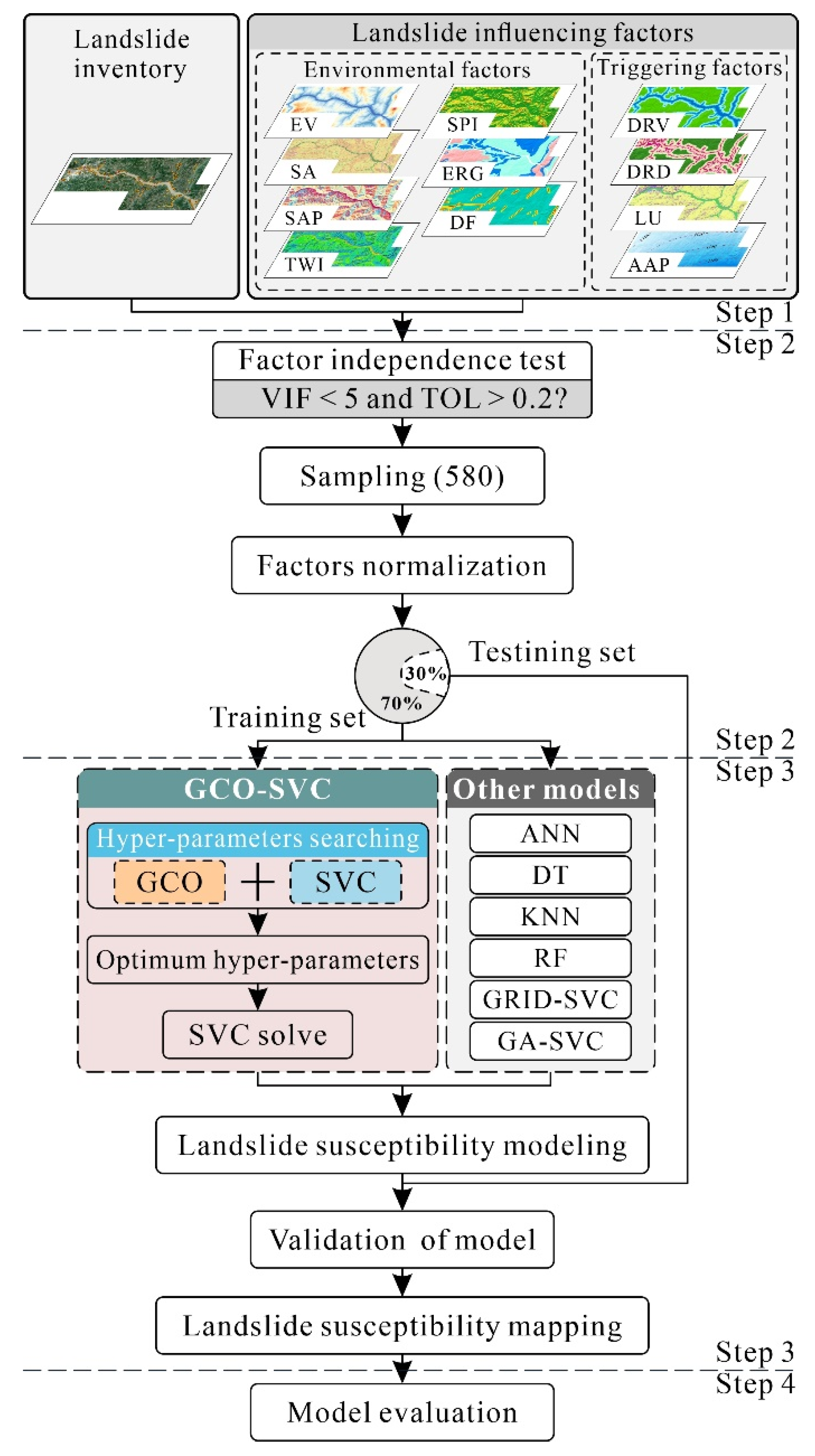
Figure 1. Flowchart.
Remotesensing 14 02707 g001
Figure 2. Location of the study area and landslide distribution. (a) Location of the TGRA in China. The base map is sourced from http://bzdt.ch.mnr.gov.cn/ (accessed on 12 January 2022). (b) Location of the study area and the landslide distribution in the TGRA. The DEM is sourced from https://search.asf.alaska.edu/ (accessed on 15 January 2022). (c) Landslide distribution in and Sentinel-2B image of the study area. The Sentinel-2B image was taken on 12 September 2021.
Remotesensing 14 02707 g002
Figure 3. Distribution of the lithology and faults in the study area. (1) Triassic thin-bedded tuffs sandwiched between shales (T1d); (2) Triassic thin-layered tuff, dolomite, gypsum, rock salt (T1-2j); (3) Triassic purplish-red mudstones, shales, and siltstones (T2b); (4) Triassic conglomerates, sandstones, slates, volcanic rocks, and limestones (T3j); (5) Jurassic yellow sandy shale, siltstone, and feldspathic quartz sandstone (J1t); (6) Jurassic purplish-red mudstone, and purplish-red mudstone sandstone interbedded (J2s1); (7) Jurassic gray-green sandstone with mudstone (J2s2); (8) Jurassic purplish-red mudstone with yellowish-gray siltstone, muddy siltstone, and feldspathic quartz sandstone (J2q); (9) Jurassic brick-red mudstone (J3s); (10) powdery clay, clayey soil, gravel layer (Qhal); (11) faults. The geologic map was obtained from the National Geological Archives of China (http://ngac.org.cn, accessed on 12 February 2022) and rendered according to the international chronostratigraphic chart (https://stratigraphy.org/chart, accessed on 12 February 2022).
Remotesensing 14 02707 g003
Figure 4. Landslide influencing factors. (a) Elevation (EV), (b) slope angle (SA), (c) slope aspect (SAP), (d) topographic wetness index (TWI), (e) stream power index (SPI), (f) engineering rock group (ERG), (g) distance to faults (DF), (h) distance to rivers (DRV), (i) distance to roads (DRD), (j) land use (LU), (k) average annual precipitation (AAP).
Remotesensing 14 02707 g004
Figure 5. Distribution of the training and testing datasets.
Remotesensing 14 02707 g005
Figure 6. GCO flowchart for optimizing the hyperparameters of RBF-SVC.
Remotesensing 14 02707 g006
Figure 7. Model performance: (a) ROC curves of the seven models on the testing set and (b) loss of the GA-SVC and GCO-SVC models.
Remotesensing 14 02707 g007
Figure 8. Landslide susceptibility maps of the seven models, includes (a) ANN, (b) DT, (c) KNN, (d) RF, (e) GRID-SVC, (f) GA-SVC, and (g) GCO-SVC.
Remotesensing 14 02707 g008aRemotesensing 14 02707 g008b
Figure 9. PFI scores of landslide influencing factors for the seven models (randomly shuffled 30 times), includes (a) ANN, (b) DT, (c) KNN, (d) RF, (e) GRID-SVC, (f) GA-SVC, and (g) GCO-SVC.
Remotesensing 14 02707 g009
Figure 10. Parameter sensitivity analysis for GCO-SVC. Model performance over different values of (a) the difficulty of mutation ( c r ), (b) the coefficient of mutation ( w f ), (c) the total population ( P o p u l a t i o n ), and (d) the number of iterations ( E p o c h ).
Remotesensing 14 02707 g010
Table 1. Multisource landslide influencing factors.
Data TypeDateInfluencing FactorsSource
DEM (12.5 m)2011Elevation (EV)
Slope angle (SA)
Slope aspect (SAP)
Topographic wetness index (TWI)
Stream power index (SPI)
ALOS PALSAR
Geologic map (1:200,000)2013Engineering rock group (ERG)
Distance to faults (DF)
National Geological Archives of China
Road network2021Distance to roads (DRD)OpenStreetMap
River network2021Distance to rivers (DRV)OpenStreetMap
Rainfall monitoring data2015–2020Average annual precipitation (AAP)Hubei Provincial Hydrology and Water Resources Bureau
Land use (10 m)2017Land use (LU)FROM-GLC10 [37]
Table 2. Kernels of the SVC model and their parameters.
Kernel NameKernel FunctionKernel Parameters
linear x , x None
poly ( γ x , x + r ) d d , γ , r
RBF exp ( γ | | x x | | 2 ) γ
sigmoid tan h ( γ x , x + r ) γ , r
Table 3. Hyperparameter search spaces of the models.
ModelParametersSearch Space
ANNNeurons in hidden layer L i n s p a c e   ( 10 ,   200 ,   10 )
L 2   penalty   parameter   ( α ) L o g s p a c e   ( 10 , 1 ,   10 )
DTMax depth L i n s p a c e   ( 1 ,   10 ,   10 )
Min sample leaf L i n s p a c e   ( 1 ,   10 )
KNNN neighbors L i n s p a c e   ( 3 ,   50 )
Weight [ u n i f o r m ,   d i s t a n c e ]
Distance [ M a n h a t t a n ,   E u c l i d e a n ]
RFNumber of estimators L i n s p a c e   ( 10 ,   200 ,   20 )
Criterion [ g i n i ,   e n t r o p y ]
GRID-SVCKernel [ l i n e a r ,   p o l y n o m i a l , R B F , s i g m o i d ]
C [ 10 3 ,   10 4 )
γ [ 10 3 ,   10 4 )
GA-SVCKernel [ l i n e a r ,   p o l y n o m i a l , R B F , s i g m o i d ]
C [ 10 3 ,   10 4 )
γ [ 10 3 ,   10 4 )
GCO-SVCKernel [ l i n e a r ,   p o l y n o m i a l , R B F , s i g m o i d ]
C [ 10 3 ,   10 4 )
γ [ 10 3 ,   10 4 )
Table 4. Multicollinearity analysis of the landslide influencing factors.
EVSASAPTWISPIERGDFDRDDRVAAPLU
VIF2.8841.9421.1232.162.0661.3931.1041.7812.9761.1231.247
TOL0.3470.5150.890.4630.4840.7180.9060.5610.3360.8910.802
Table 5. The optimal hyperparameters of the seven models.
ModelParameter SettingsOptimal HyperparametersBest Score
ANN M a x I t e r a t i o n s = 500
S o l v e r = l b f g s
H i d d e n L a y e r S i z e = 70
α = 0.1
0.434876
DT C r i t e r i o n = g i n i
S p l i t t e r = b e s t
M a x D e p t h = 2
M i n S a m p l e s L e a f = 1
0.324234
KNN A l g o r i t h m = a u t o
L e a f S i z e = 30
n N e i g h b o r s = 23
W e i g h t s = d i s t a n c e
D i s t a n c e = M a n h a t t a n
0.290551
RF M a x D e p t h = N o n e
M i n S a m p l e s S p l i t = 2
M i n S a m p l e s L e a f = 1
n E s t i m a t o r s = 135
C r i t e r i o n = g i n i
M a x F e a t u r e s = l o g 2
0.238102
GRID-SVC C o e f 0 = 0
T o l = 0.0001
M a x I t e r a t i o n s = 1
C = 1.0
γ = 0.1
K e r n e l = r b f
0.243250
GA-SVC C o e f 0 = 0
T o l = 0.0001
M a x I t e r a t i o n s = 1
E p o c h = 100
P o p u l a t i o n = 100
c p = 0.95
m p = 0.025
C = 0.46565951
γ = 0.15258858
K e r n e l = r b f
0.232593
GCO-SVC C o e f 0 = 0
T o l = 0.0001
M a x I t e r a t i o n s = 1
E p o c h = 100
P o p u l a t i o n = 100
c r = 0.70
w f = 1.25
C = 0.64040679
γ = 0.19201292
K e r n e l = r b f
0.231471
Table 6. Model performance on the training and testing sets.
DatasetMetricANNDTKNNRFGRID-SVCGA-SVCGCO-SVC
TrainingAccuracy1.00000.89661.00001.00000.94090.93840.9532
F1 score1.00000.89811.00001.00000.94200.94000.9538
Log loss0.00003.57300.00000.00002.04172.12681.6164
AUC1.00000.89651.00001.00000.94080.93820.9532
TestingAccuracy0.90800.89080.89660.90800.91950.93680.9425
F1 score0.90360.89140.89890.90800.91860.93640.9412
Log loss3.17603.77153.57303.17602.77902.18351.9850
AUC0.90750.89140.89760.90850.91980.93710.9425
Table 7. Pairwise comparison results for the seven models using the Wilcoxon signed-rank test (two-tailed).
Pairwise Comparison z Value p ValueSignificance
GCO-SVC vs. ANN333.560.00Yes
GCO-SVC vs. DT−160.030.00Yes
GCO-SVC vs. KNN−515.590.00Yes
GCO-SVC vs. RF−8.670.00Yes
GCO-SVC vs. GRID-SVC81.970.00Yes
GCO-SVC vs. GA-SVC333.790.00Yes
Table 8. Density analysis of landslide susceptibility maps of the different models.
ModelSusceptibility LevelPixels in Domain (A)Pixels in Landslide (B)Percentage of Domain to Total Domain (C)Percentage of Landslide to Total Landslide (D)Frequency Ratio (D/C)
ANNVery Low1,006,570322278.19%9.55%0.1221
Low44,61010583.47%3.13%0.9046
Moderate24,9667911.94%2.34%1.2084
High37,50416552.91%4.90%1.6831
Very High173,61927,02513.49%80.07%5.9368
DTVery Low1,012,900491178.69%14.55%0.1849
Low000.00%0.00%0.0000
Moderate73,69133255.72%9.85%1.7209
High101,85686837.91%25.73%3.2514
Very High98,82216,8327.68%49.87%6.4963
KNNVery Low653,4248150.76%0.24%0.0047
Low207,63072616.13%2.15%0.1334
Moderate131,899162710.25%4.82%0.4705
High172,609825413.41%24.46%1.8238
Very High121,70723,0639.45%68.33%7.2274
RFVery Low819,929112863.70%3.34%0.0525
Low201,461242015.65%7.17%0.4581
Moderate88,13330106.85%8.92%1.3026
High75,98959445.90%17.61%2.9834
Very High101,75721,2157.90%62.86%7.9517
GRID-SVCVery Low900,588118569.96%3.51%0.0502
Low116,04016509.01%4.89%0.5423
Moderate58,30318094.53%5.36%1.1834
High79,55144406.18%13.16%2.1287
Very High132,78724,66710.32%73.09%7.0851
GA-SVCVery Low919,184133771.41%3.96%0.0555
Low101,45514927.88%4.42%0.5609
Moderate53,74216524.17%4.89%1.1724
High73,13841035.68%12.16%2.1396
Very High139,75025,16710.86%74.57%6.8685
GCO-SVCVery Low918,028133171.32%3.94%0.0553
Low106,41714988.27%4.44%0.5369
Moderate51,98116384.04%4.85%1.2019
High69,34840445.39%11.98%2.2241
Very High141,49525,24010.99%74.78%6.8035
Publisher’s Note: MDPI stays neutral with regard to jurisdictional claims in published maps and institutional affiliations.