Article

Choosing the Right Horizontal Resolution for Gully Erosion Susceptibility Mapping Using Machine Learning Algorithms: A Case in Highly Complex Terrain

1
Shaanxi Key Laboratory of Earth Surface System and Environmental Carrying Capacity, College of Urban and Environmental Sciences, Northwest University, Xi’an 710127, China
2
Key Laboratory of National Forestry Administration on Ecological Hydrology and Disaster Prevention in Arid Regions, Northwest University, Xi’an 710127, China
3
Department of Agronomy, Iowa State University, Ames, IA 50011, USA
*
Author to whom correspondence should be addressed.
Remote Sens. 2022, 14(11), 2580; https://doi.org/10.3390/rs14112580
Submission received: 23 April 2022 / Revised: 19 May 2022 / Accepted: 25 May 2022 / Published: 27 May 2022

Abstract

:
Gully erosion susceptibility (GES) maps are essential for managing land resources and erosion control. Choosing the optimal horizontal resolution in GES mapping is a challenge. In this study, the optimal resolution for GES mapping in a complex loess hilly area on the Chinese Loess Plateau was tested using two machine learning algorithms. Unmanned aerial vehicle (UAV) images with a 9 cm resolution and GNSS RTK field-measured data were employed as base datasets, and 11 factors were used in the machine learning models. A series of horizontal resolutions, from 0.5–30 m, was used to determine which was the optimal level and how the resolution influenced the GES mapping. The results showed that the optimal resolution for GES mapping was 2.5–5 m in the loess hilly area, for both the random forest (RF) and extreme gradient-boosting (XGBoost) machine learning algorithms employed in this study. High resolutions overestimated the probability of gully erosion in stable regions, and it became difficult to identify gully and non-gully regions at too-coarse resolutions. The variable importance for GES mapping changed with the resolution and varied among variables. Slope gradient, land use, and contributing area were, in general, the three most critical factors. Land use remained an important factor at all the tested resolution levels. The importance of the slope gradient was underestimated at coarse resolutions (10–30 m), and the importance of the contributing area was underestimated at resolutions that were comparatively fine (0.5–1 m). This study provides an essential reference for selecting the optimal resolution for gully mapping, and thus, offers support for approaches attempting to map gullies using UAV.

Graphical Abstract

1. Introduction

Gully erosion is one of the most severe types of soil erosion [1,2] and is a threat to the environment and society [3]. It affects nearly 1 billion hectares of land worldwide [4], and its soil loss rate accounts for 10–94% of the total sediment production caused by water erosion [5]. The gully erosion susceptibility (GES) map is a valuable tool for discovering potential gully-prone areas and, thus, for helping to control gully erosion [6,7]. The selection of resolution affects the accuracy of the modeling results, making the selection of the optimal resolution one of the major challenges in GES mapping.
In previous studies, topographic thresholds, traditional statistical models, and machine learning algorithms are usually used to predict gully location. Machine learning algorithms, such as random forest (RF) [3,8], support vector machine (SVM) [9,10], boosted regression tree (BRT) [9,11], multivariate additive regression Spline (MARS) [3,8] and gradient-boosted regression tree (GBRT) [12], do not require common assumptions regarding parameter statistics and provide high-precision simulation results, and they are widely used in GES mapping to evaluate the probability of gully occurrence. In these algorithms, the RF algorithm has been applied in a wide range of applications and provides high simulation accuracy [3,9,12]. The more advanced extreme gradient-boosting (XGBoost) algorithm was recently applied and yielded good simulation results [13,14,15].
Factors such as topography, lithology, soil features, climate, hydrology, land use (LU), and vegetation cover can affect the process and distribution of gully erosion; therefore, these factors and related variables are usually used as independent variables in GES mapping [16]. The effect of factors on gully erosion is not constant. As studies by Rahmati et al. [11] and Arabameri et al. [17] have shown, hydrology is the most critical factor affecting GES mapping in northern Iran. Research by Gayen et al. [3] suggested that LU is the most important factor in the Pathro River Basin of eastern India. Jiang et al. [18] and Yang et al. [14] found that topography is the most critical factor in the Loess Plateau region. Chowdhuri et al. found that Normalized Difference Vegetation Index (NDVI) was the most critical factor in the eastern fringe area of the Chota Nagpur plateau. The sources of data associated with these factors are extensive. Data for topographical and hydrological factors are mainly obtained from topographical maps at various scales, the advanced land-observing satellite (ALOS) DEM, and the advanced spaceborne thermal emission and reflection radiometer (ASTER) DEM. LU and vegetation cover data are mainly obtained from Sentinel-2A and Landsat images. Lithology and soil feature data are mainly obtained from geological and soil maps at various scales. Therefore, most studies produce GES maps at medium and low resolutions (10–30 m). In recent years, unmanned aerial vehicles (UAVs) and light detection and ranging (LIDAR) technology have been used for mapping at finer resolutions.
With the broad application of machine learning algorithms and various data sources, performing accurate GES mapping has become an urgent task. The horizontal resolution of data affects the detection and analysis of land surface features [19]. DEM and remote sensing data at different resolutions can be used to identify various topographical, hydrological, and environmental factors to use as GES mapping parameters. Testing the influence of resolution on GES mapping helps researchers understand the uncertainty of gully erosion modeling and improves the mapping accuracy of the models [20]. Some studies have suggested that the finer the resolution, the higher the accuracy of the GES mapping. Lucà et al. [21] compared the impact of the resolution from 7.5 to 20 m on GES mapping. They found that the larger the spatial resolution was for influential variables, the lower the mapping accuracy and the extent of the most-susceptible classes. Other studies have suggested that very-fine resolutions may not necessarily yield the best GES mapping accuracy. For example, Gomez-Gutierrez et al. [22] compared the impact of the resolution of 2 to 50 m on GES mapping and noted that the optimal resolution in the San Giorgio basin and the Mula River basin was 4 m and 20 m, respectively. The selection of resolution should be related to the size of the landform. Garosi et al. [23] found that a resolution of 10 m was most-suitable for GES mapping in the Ekbatan Dam Basin, based on the resolution of 2 to 30 m. The gullies with high cross-sectional areas partly influenced the optimal resolution. Therefore, scholars have different views on the influence of resolution on GES mapping, and the optimal resolution in different regions is often variable. The range of the detected resolution and the gully size may affect the judgment of the optimal resolution. Additionally, most study areas have been relatively flat (e.g., areas in Italy, Spain, and Iran), and the optimal resolution has not been tested in complex-terrain areas.
In recent years, the rapid development of UAV technology has made it very convenient to obtain fine and diverse resolution data, and has greatly improved the detectable range of resolution. In the Loess Plateau of China, the terrain is highly complex, and most of the gullies are distributed on steep hillslopes. The expression of gully features may require fine resolutions [24].
This study aims to evaluate the impact of horizontal resolution (0.5–30 m) on GES mapping in loess hilly regions where the terrain is highly complex. The results of this study may provide a reference for selecting the optimal resolution for the GES mapping and provide support for gully erosion management.

2. Materials and Methods
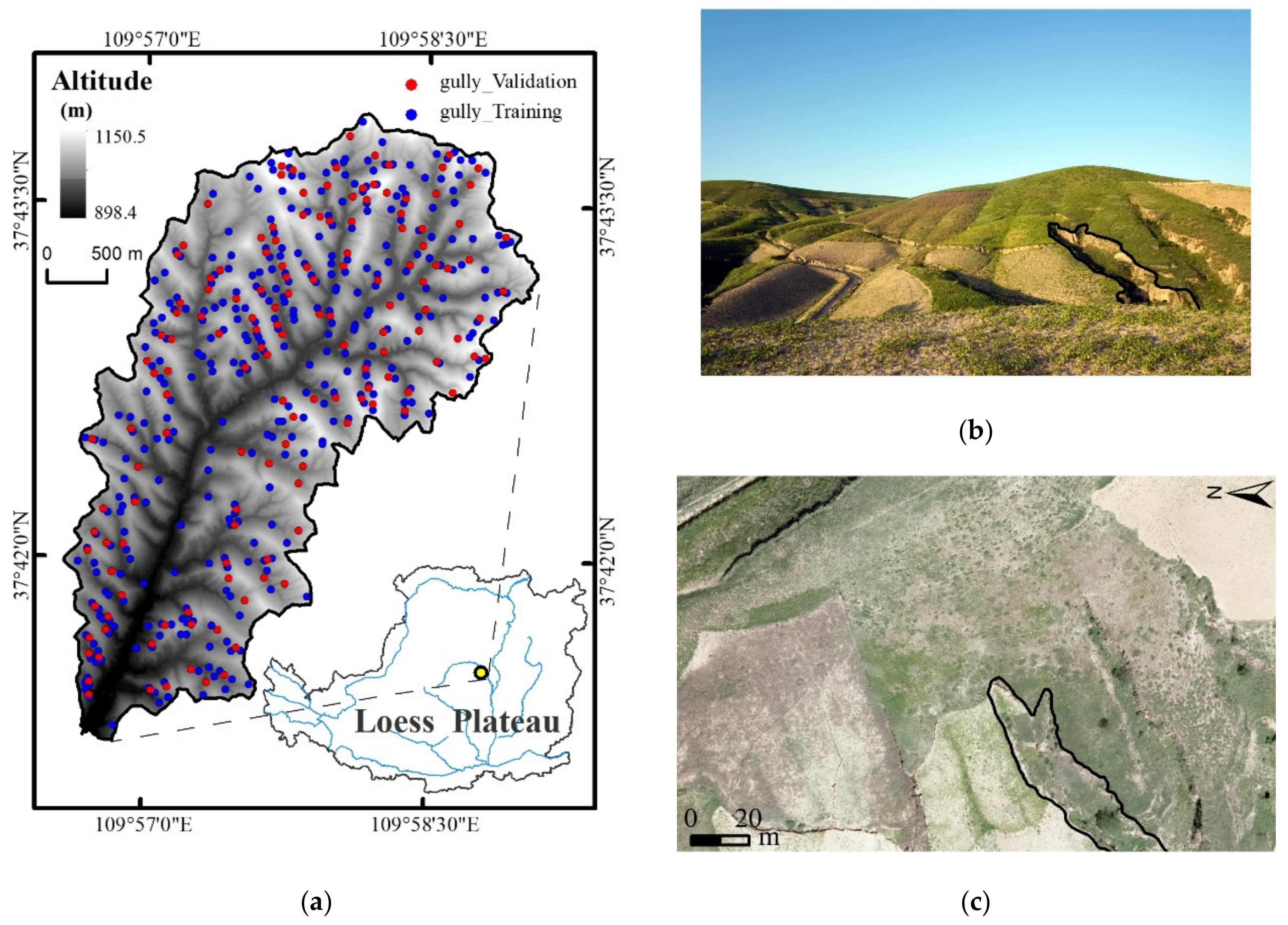
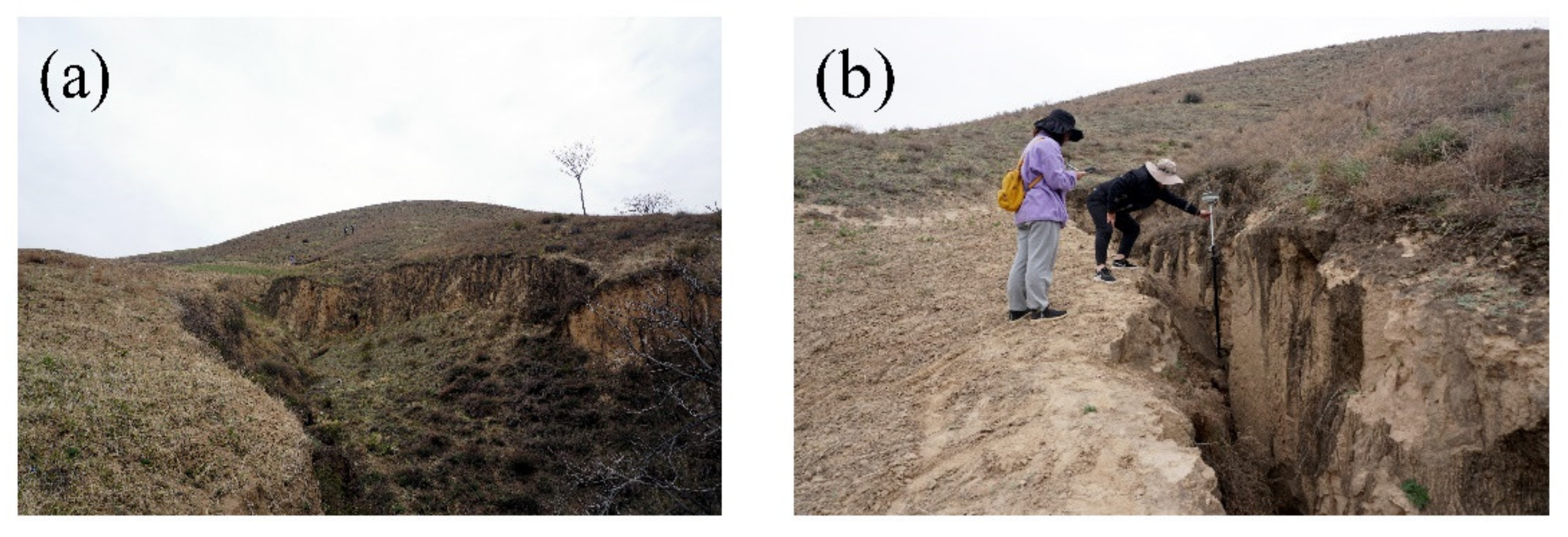
2.1. Study Area

The study area is the Mizhigou watershed (37°41′ to 37°43′N, and 109°56′ to 109°59′E), with an area of 10.9 km2. This watershed is located in Shaanxi Province, a typical loess hilly area (Figure 1). The average yearly precipitation is 430 mm; most of the rainfall occurs from May to September, with heavy rains and frequent floods. The natural vegetation in the study area is mainly herbaceous, with small quantities of shrubs and trees. The height of vegetation is relatively homogeneous. The LU types are mainly grassland (67%) and agricultural land (23%). The terrain here is highly complex. The average slope gradient is 28.7°, and 27.1% of the hillslopes are steeper than 40°. The main soil type is loess, with silt size particles. This kind of soil is characterized by weak cohesion, high infiltrability, low water retention, and high erodibility [25]. Gullies are widely distributed in the study area.

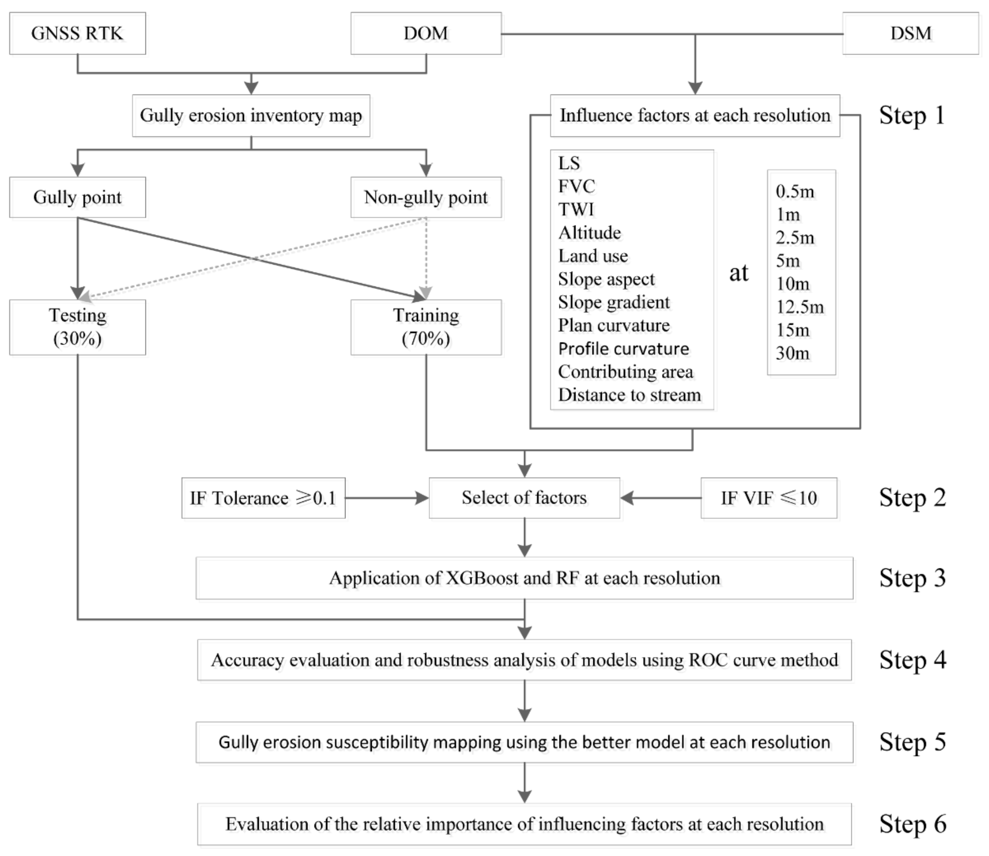
2.2. Experimental Procedure

The experimental process includes the following six steps; see Figure 2. Step 1 involves the acquisition of base data, including the gully erosion inventory map and data for the factors that influence gully erosion at various resolutions. Step 2 is a multicollinearity analysis, which ensures that the factors involved in the machine learning modeling are independent of each other. Step 3 is building the ML model at various resolutions, and the algorithms used in this step are RF and XGBoost. Step 4 involves using the receiver operating characteristic (ROC) curve to evaluate the accuracy of each model and to evaluate the robustness of the models at the optimal resolution. Step 5 includes generating GES maps at each resolution using the optimal model. In Step 6, the relative importance of each influential factor is determined at each resolution. In our previous study [14], when calculating the weight of factors based on the Gini index, the results obtained by RF and XGBoost were consistent. Therefore, we decided to choose a model with higher simulation accuracy to obtain the variable importance.

2.3. Base Datasets and Data Processing

We used a UAV to obtain digital surface models (DSMs) and digital orthophoto maps (DOMs) of the studied watershed in August 2019 at a spatial resolution of 9 cm. The type of UAV used was a DJI4RTK, and control points were evenly distributed in the study area to reduce the position offset error and increase the accuracy of data [26]. The flying altitude of the UAV was 300 m, and the side overlap and front overlap were both more than 70%. The weather conditions were good, with a clear, partly cloudy sky. The Pix4D mapper software was used for data processing. Firstly, the acquired image was matched and calibrated. Then, point clouds were generated from the calibrated image to create the 3D mesh, and a 3D model was built using the SfM method to generate a DOM and DSM. Based on the DSM, a series of DEMs with various resolutions (0.5, 1, 2.5, 5, 10, 12.5, 15, and 30 m) was obtained.

2.4. Gully Erosion Inventory Mapping

A gully erosion inventory map shows the location of gullies, and is the basis for the spatial modeling of gully erosion [11]. It was mainly obtained from a visual interpretation based on a 9 cm DOM in this study. Our previous research [14] showed that the gully erosion inventory mapping accuracy using UAV images was 96.78%, according to the field-measured results using GNSS RTK (Figure 3). In this study, 482 gully polygons were randomly selected, of which 337 (70%) were randomly selected as the training set for GES map modeling, and the remaining 145 (30%) were used for model validation. Non-gully polygonal regions were randomly selected to generate the same number of training and testing sets in the watershed.
The length of these gullies ranged from a few meters to several hundred meters, and the width ranged from a few meters to dozens of meters. The average length was approximately 50 m, and the average width was approximately 15 m. Most of the gullies are connected downstream of the drainage network, and the sediment produced by gully erosion is quickly transported to other areas via the drainage network.

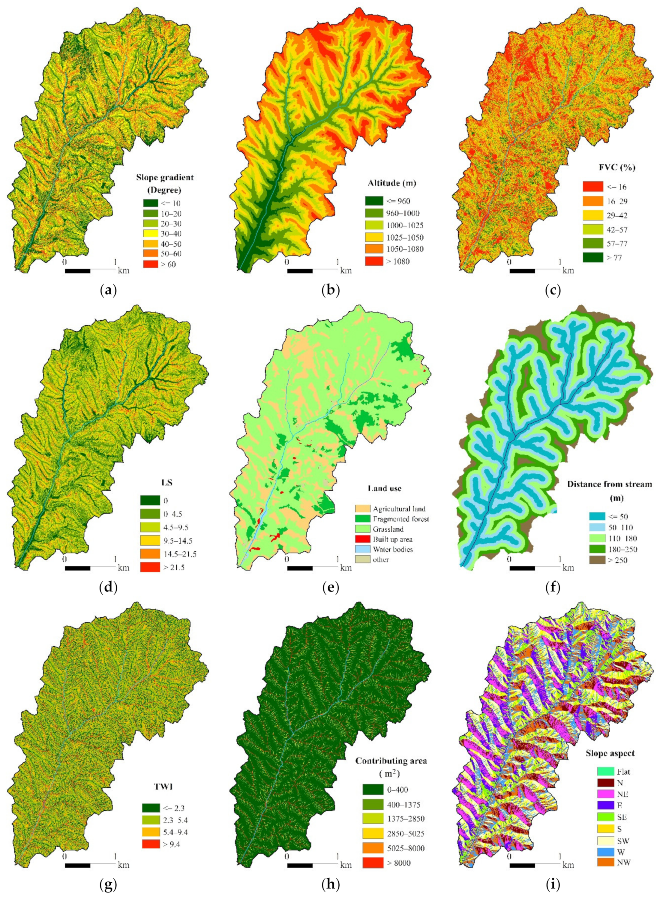
2.5. Factors That Influence Gully Erosion

The selection of influential factors is a critical step in GES map modeling, and it directly affects the quality of the model and prediction accuracy [27,28]. Topographical, environmental, hydrological, geological, and climatological conditions affect the initiation and development of gully erosion. However, global consensus and standard methods for selecting these factors have not yet been established [29]. Based on previous studies [9,30,31], topographical, hydrological, and environmental factors were generally considered as the most critical factors affecting gully erosion. Therefore, we selected altitude, slope gradient (Slope), slope aspect (Aspect), plane curvature (PlC), profile curvature (PrC), contributing area (CA), slope length and steepness (LS), topographical wetness index (TWI), distance from streams (D_stream), land use (LU), and fractional vegetation cover (FVC) as parameters for GES mapping. The topographic factors were obtained based on the DEMs at various resolutions. The other factors, at varied resolutions, were obtained by resampling their highest-resolution datasets (Figure 4).
Specifically, we used surface analysis tools in the software ArcGIS 10.5 to generate topographic factors, including slope gradient, slope aspect, plane curvature, and profile curvature. We also used hydrological analysis tools to calculate the contributing area using the same software. Land use and streams datasets were obtained from a visual interpretation based on DOM, and the distance from streams was generated based on the Euclidean distance tool in the software ArcGIS 10.5. LS and TWI were obtained according to the algorithms provided by Zhang et al. [32] and Moore et al. [33], respectively. FVC was calculated from the visible-band difference vegetation index (VDVI) (Equation (1)), based on UAV-sourced DOMs. The value range of VDVI is [−1, 1]; it can be calculated according to Equation (2) [34]:
FVC = VDVI     VDVI soil   / ( VDVI veg   VDVI soil )
VDVI = 2   ×   ρ green   ρ red   ρ blue 2   ×   ρ green + ρ red + ρ blue
where ρ green , ρ red , and ρ blue are the values of the green band, red band, and blue band, respectively. VDVI soil and VDVI veg are the VDVI values of bare soil and dense vegetation, respectively. The 5th and 95th percentile of the VDVI value were used as VDVI soil and VDVI veg , respectively.
We used ArcPy to realize the automatic extraction of influence factors; it is very convenient for repetitive and cumbersome data processing tasks and can achieve a variety of processing work, such as geographic data management, data transformation, and data analysis.

2.6. Multicollinearity of the Factors That Influence Gully Erosion

In a multiple regression model, incorrect prediction results will be obtained when there is a linear relationship between two or more independent variables in the dataset; therefore, it is usually necessary to perform a collinear analysis among the influential factors before modeling [35]. When there is a high correlation between two variables in the dataset, those specific variables need to be removed. Tolerance and variance inflation factor (VIF) are two indexes used to evaluate collinearity among variables. In general, for the collinearity values of TOL < 0.1 and VIF > 10 [17], the corresponding formulas are:
Tolerance = 1     R j 2
VIF = 1 Tolerance
where R j 2 represents the coefficient of determination of explanatory variable j in the regression based on all the other explanatory variables.

2.7. Description of the Models

2.7.1. Random Forest (RF)

RF is a nonparametric multivariable model based on multiple decision trees. It is commonly used in classification and regression tasks and can be applied for variable selection, clustering, and interaction detections [11,36]. It is an effective method to solve the problem of nonlinear higher-dimensional GES assessment. The RF algorithm generates several weak classifiers based on decision trees by replacing and continuously changing the factors that affect the target. Then, the final prediction results are output through a comprehensive analysis of these weak classifiers. The prediction results of RF classification are obtained via the simple majority voting method, and the results of RF regression are obtained by calculating the average value of each classifier. The main advantages of the RF model are as follows: (1) there is no need for assumptions about the data distribution; (2) overfitting is avoided; (3) each subtree is constructed by randomly selecting a certain number of data and features, the correlations among the features of a single tree are very low, and the RF system is highly diverse; (4) estimation errors are minimized by using out-of-bag (OOB) data; (5) the output results are obtained by averaging over a large number of trees, with low deviation and variance; and (6) excellent prediction performance can be achieved [37].
The RF modeling process was implemented in Python 3.8. In the modeling process, the number of trees, the number of factors, and the number of nodes are considered to be hyperparameters that need to be tuned, and they control the complexity of the model. Complex models often need more computing memory and time. The best model was determined by using five-fold cross-validation.

2.7.2. Extreme Gradient Boosting (XGBoost)

XGBoost is an algorithm based on an improvement to traditional gradient boosting, which was initially proposed by Chen and Guestrin [38]. XGBoost has won many data science competitions and is one of the most advanced methods in machine learning. Notably, it has been one of the most widely used algorithms in recent years [13,39]. Individual decision trees are serially trained so that each tree is an improved version of the previous one, thus reducing the residuals and the error rate [40]. XGBoost includes several sub-algorithms, such as sparsity-aware split finding, approximation, basic exact greedy, and weighted quantile sketch procedures, which can efficiently determine the best splitting. To avoid overfitting, XGBoost also introduces regularization to limit the complexity of trees. Some models perform well in the training set but poorly in testing, indicating that the model’s generalization ability is poor. The addition of regularization helps overcome overfitting problems and improves the flexibility of the gully erosion prediction model. In addition to regularization, shrinkage and column subsampling are also used to prevent overfitting in XGBoost. Moreover, XGBoost provides scalability, sparse data processing, comprehensive document availability, low computing resource requirements, and high performance for different scenarios, and it is easy to implement [38]. XGBoost aims at minimizing the following objective function:
Obj = i = 1 m l   y i , y ^ i + k = 1 K Ω f k
The first term in this equation represents the loss function, which measures the difference between the actual value ( y i ) and the predicted value ( y ^ i ), and the second one controls the model complexity to avoid overfitting. Minimizing this objective function helps to reduce generalization errors and improves computational efficiency.
In this study, XGBoost was implemented using the XGBoost Python packages in the Python 3.8 environment. In the modeling process, the number of trees was set to 250, and the other hyperparameters (e.g., max_depth, eta, gamma, lambda, alpha, colsample_bytree, colsample_bynode) were tuned by using five-fold cross-validation.

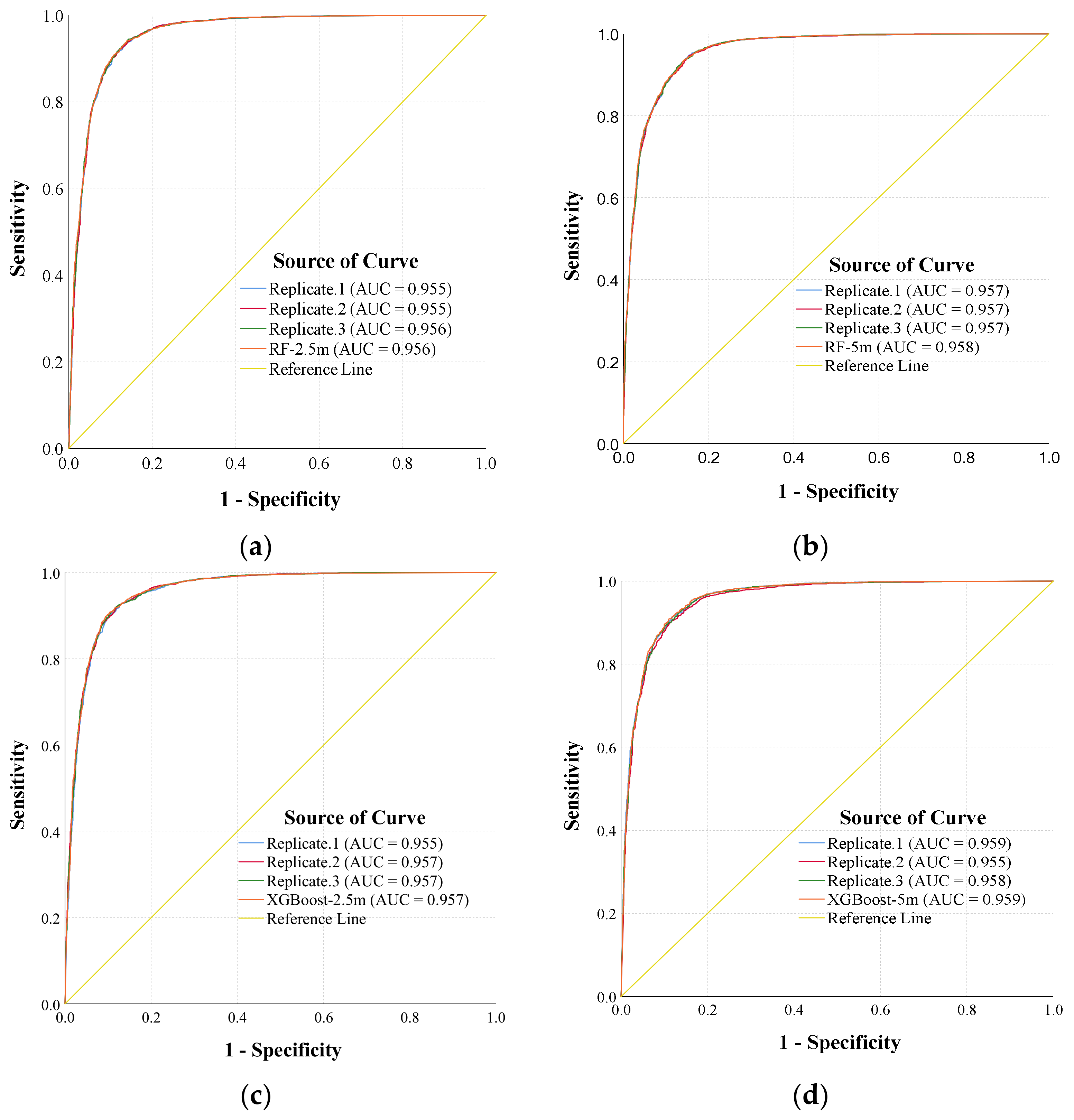
2.8. Validation of the Modeling Results

The ROC curve method is used to assess probability prediction and statistical prediction systems, and it has been widely used to evaluate the accuracy of models [41,42]. The shape of the ROC curve represents the accuracy of the model, and an ROC curve near the upper-left corner suggests that the accuracy of the model is high. Additionally, the area under the curve (AUC) can be used to evaluate the advantages and disadvantages of a model quantitatively, and an AUC = 0.5 suggests that the prediction effect of the model is poor and at a level no better than random identification, for gully and non-gully pixels in this case. An AUC = 1 indicates that the model can perfectly predict gully and non-gully pixels [43]. The quantitative–qualitative relationship between the AUC value and prediction accuracy is as follows: 0.5–0.6 is poor, 0.6–0.7 is average, 0.7–0.8 is good, 0.8–0.9 is very good, and 0.9–1 is excellent [8]. In addition, after determining the optimal pixel size, the training and testing sets obtained for the best pixel size are changed three times to evaluate the robustness of the model. The AUC can be calculated by the following equations:
TPR = TN TP + FN
FPR = TN FP + TN
AUC = TP + TN P + N
where TP is a true positive, TN is a true negative, FP is a false positive, and FN is a false negative. P and N represent the presence and absence of gullies, respectively.

3. Results

3.1. Analysis of the Multicollinearity of Factors

Table 1 presents the collinear analysis results for each factor at various resolutions. The minimum value of tolerance and the maximum value of VIF were 0.15 and 6.56, respectively. These values indicate that there is no collinearity among the factors selected at various resolutions, and that all factors can be used in GES mapping.

3.2. Impacts of Resolution on Modeling Accuracy

Figure 5 displays the predictive performance of the models at each resolution. The results showed that with the coarsening of the resolution, the AUC increased at first and then decreased, with a maximum value at a resolution from 2.5 m to 5 m. This finding indicates that the finest resolution does not necessarily yield the best mapping accuracy, and medium resolutions are often the best. Additionally, different algorithms do not affect the selection of the optimal resolution. Notably, the overall AUC of XGBoost was higher than that of the RF algorithm, especially when the resolution was lower than 10 m. Thus, the XGBoost algorithm is more suitable for mapping in the study area.
To verify the robustness of the models, we randomly selected three different samples from the training and testing sets to evaluate the prediction accuracy at a resolution of 2.5–5 m (Figure 6). The results showed that the maximum difference of the AUC in different random samples was less than 0.04. Thus, the two models exhibit good stability for three random samples, and the results are similar.

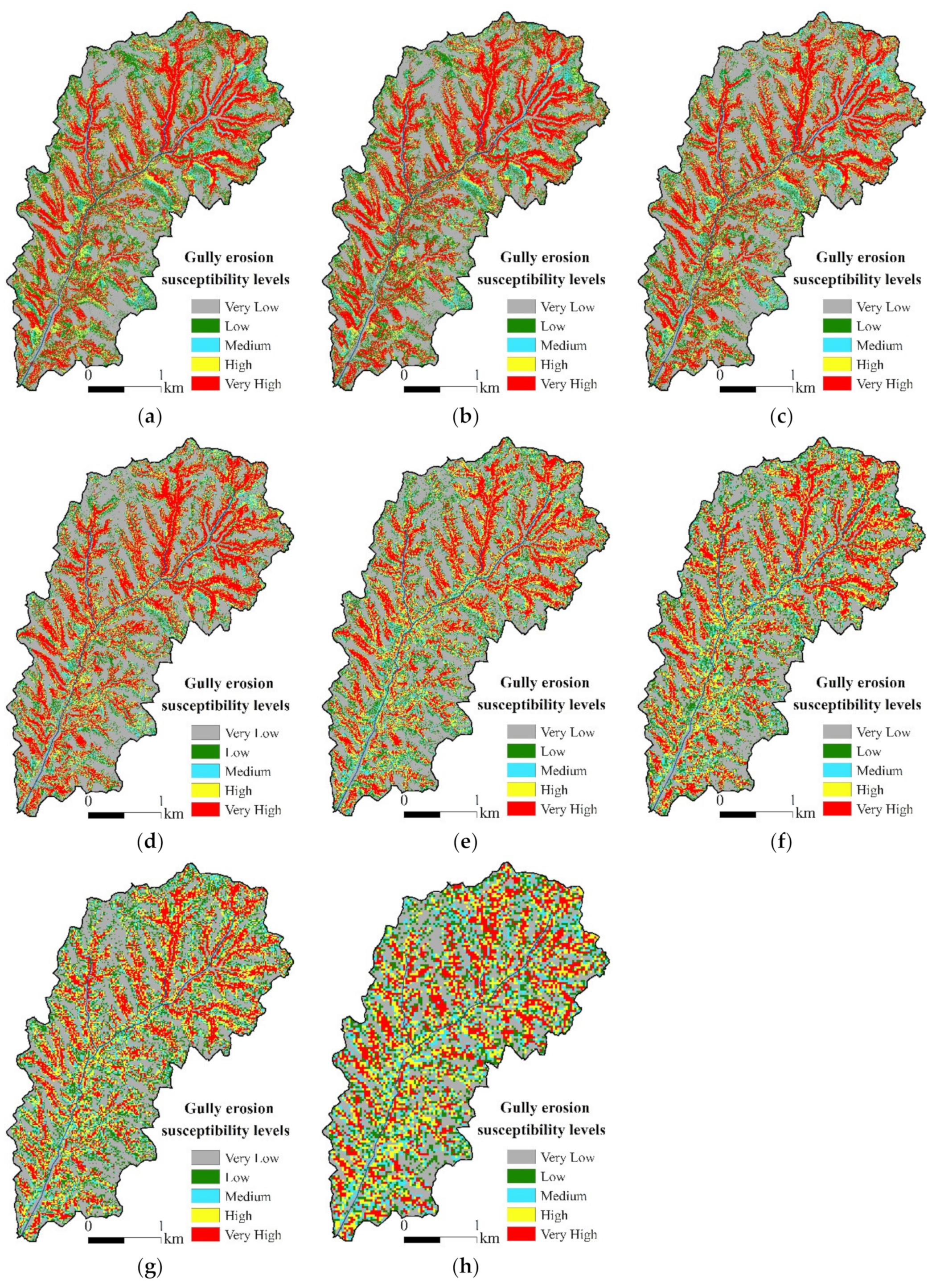
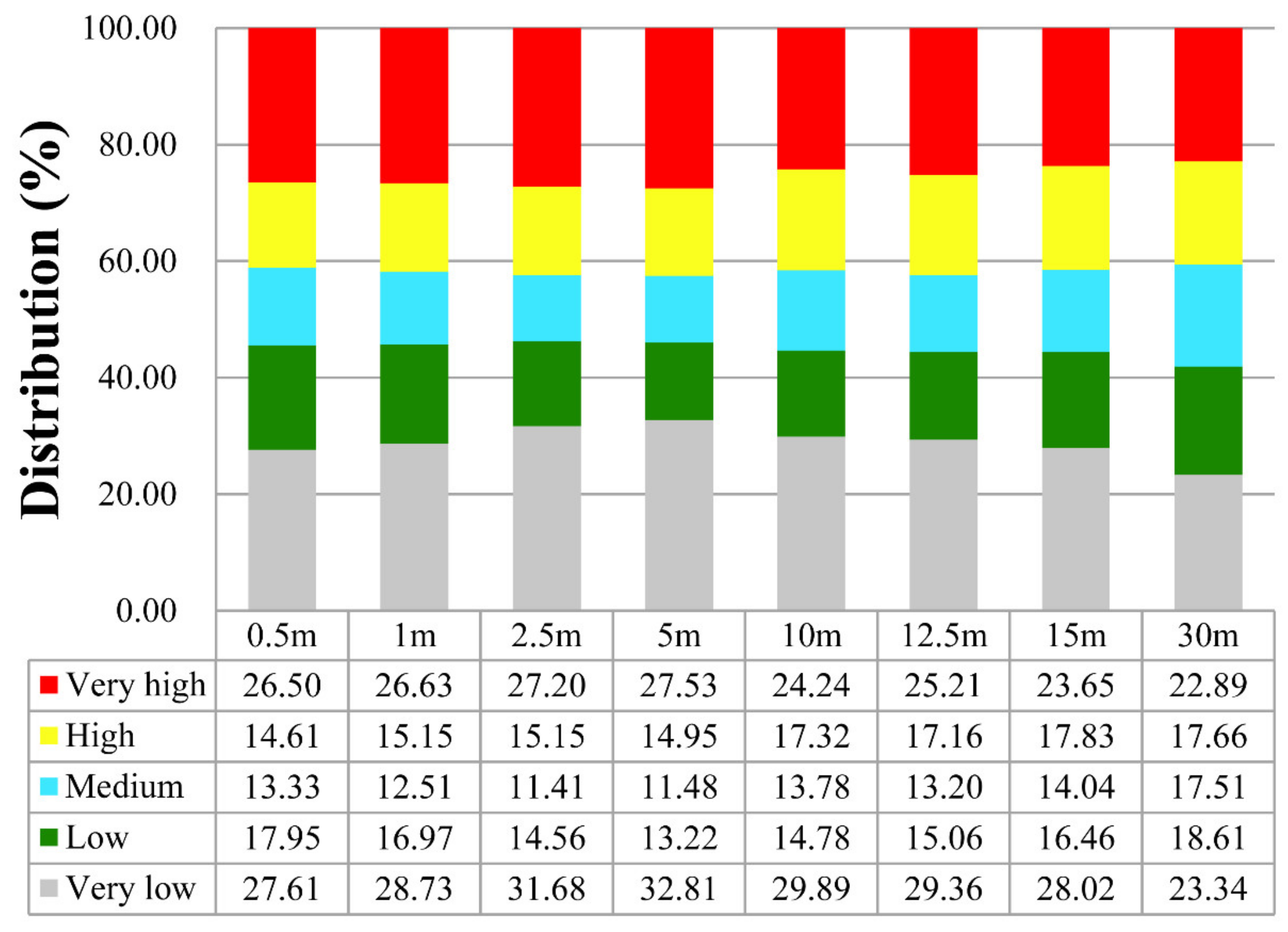
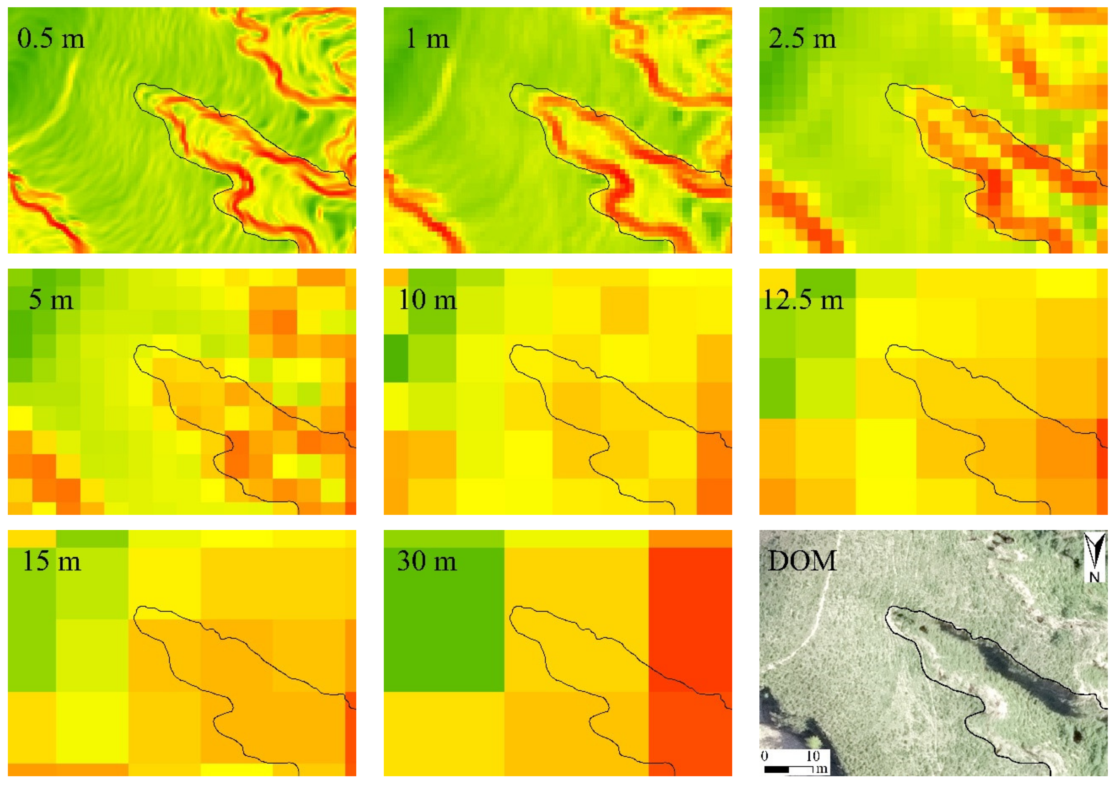
3.3. Impacts of Resolution on GES Map

Based on the XGBoost algorithm, we created a GES map at each resolution and used the natural breaks method to divide erosion areas in each map into five different classes: “very low”, “low”, “medium”, “high”, and “very high” susceptibility (Figure 7). The prediction of the very high- and high-susceptibility classes was consistent in the GES maps at resolutions of 0.5–5 m. These areas were mainly distributed on both sides of stream banks, in the middle of hillslopes, and in areas closely connected to the drainage network. Notably, the classification of very low-susceptibility areas greatly varied. It had a smaller range when the resolution was fine (0.5–1 m). The continuity of the 10–30 m map was poor, and with the coarsening of the resolution, the maps became increasingly fragmented.
Figure 8 quantitatively shows the percentages of susceptibility classes at each resolution. The percentages of both the very high- and high-susceptibility classes did not change much with a resolution ranging from 0.5 to 5 m. The model at this resolution is consistent with gully simulation, and the area is seriously affected by gully erosion. The very low-susceptibility class was more affected by the resolution. At fine resolution (0.5–1 m), the percentage of this class was low, and more areas were predicted to be low- and medium-susceptibility classes. When the resolution became coarser, from 5 m to 30 m, generally speaking, the percentages of the very low- and very high-susceptibility classes both decreased, and more areas were predicted to be moderately susceptible. This result indicates that, as the resolution becomes coarser, the ability of the model to distinguish between gully and non-gully areas decreases.

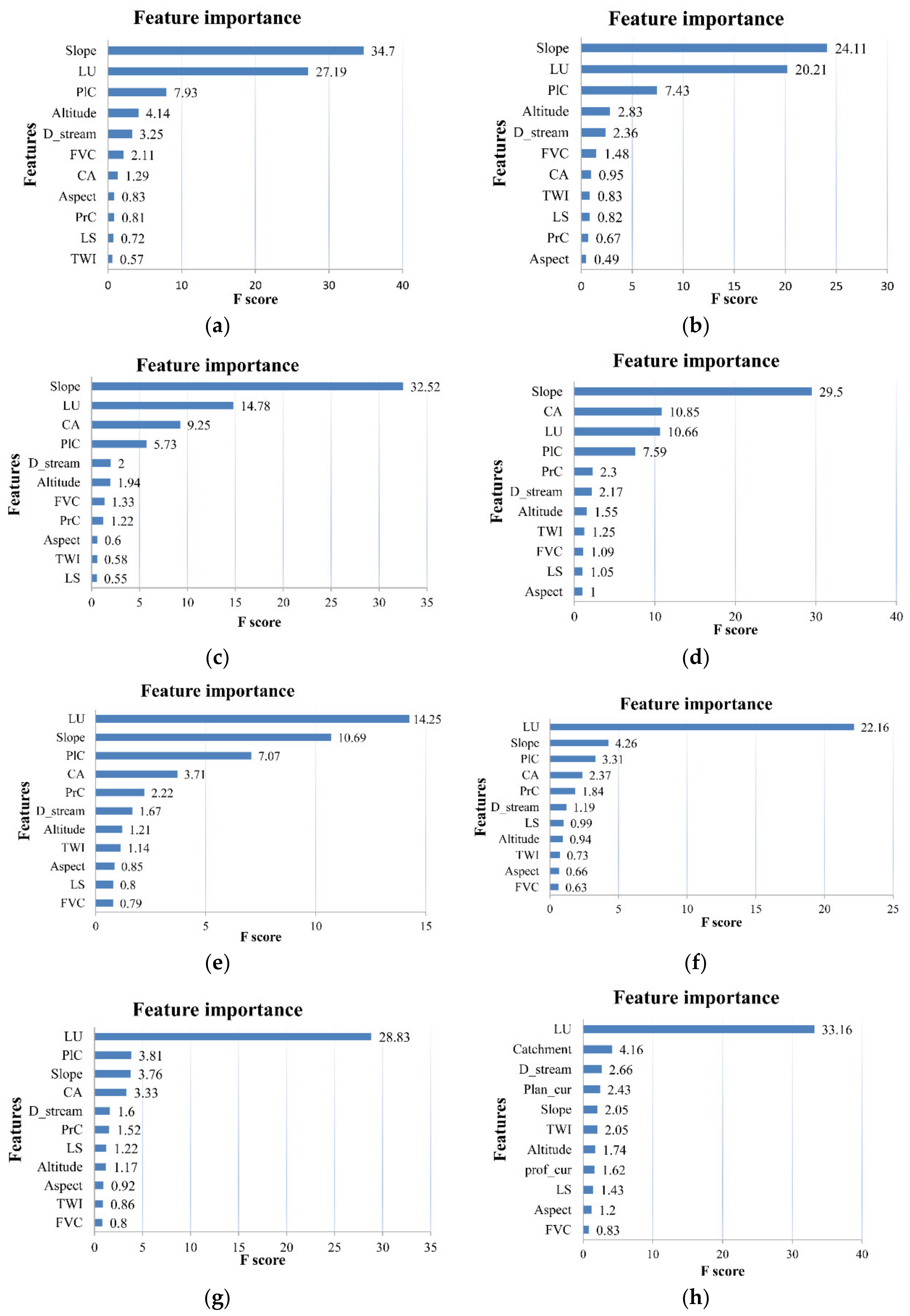
3.4. Impacts of Resolution on Variable Importance

Figure 9 illustrates the relative importance of the influential variables at each resolution. The greater the F-score, the greater its role in GES mapping, and the closer its relationship with gully erosion. The results suggested that the slope gradient, LU, contributing area, and plane curvature were the most critical variables, and their importance was different at various resolutions. When the resolution was relatively fine (0.5–1 m), the relative importance of the contributing area decreased, and altitude was a relatively important factor. When the resolution was relatively coarse (10–30 m), the relative importance of the slope gradient decreased, and LU gradually became the dominant factor.

4. Discussion

4.1. Exploration of the Optimal Resolution

GES maps differed at various resolutions. There was little difference between the distribution and percentages of the very high- and high-susceptibility classes at fine resolution (0.5–5 m). At the finest resolution (0.5–1 m), the very low-susceptibility class decreased significantly in abundance, and more areas were classified as low- and medium-susceptibility areas. Thus, gully features were not well-expressed at fine resolutions, and susceptibility was overestimated in some stable areas where no gullies are located and the terrain is relatively flat (Figure 4i). At coarse resolutions (10–30 m), the percentages of the very low- and very high-susceptibility classes gradually decreased, and the maps became increasingly fragmented. Notably, although the local variance is reduced at coarse resolutions and the influence of detailed land surface information is limited, gully features are often overgeneralized [44], thus narrowing the gap between gully and non-gully areas on hillslopes. The average size of gullies in this study is relatively small. With the coarsening of the resolution, the number of gully pixels decreased, and some gully information was difficult to express. The features of objects must be many times larger than the spatial resolution to be consistently and accurately recognized [45]. Therefore, in the process of mapping, not only should the landform features be effectively expressed, but the impact of detailed land surface information should also be avoided in flat areas.
The properties of terrain and gullies may affect the selection of the optimal resolution. Gorasi et al. [23] found that the optimal resolution of GES mapping in the Ekbatan Dam Basin was 10 m, based on four machine learning models. The average slope gradient of the ground is an important index to measure the terrain complexity [46]. In this study, the average slope gradient was 28.7°, greater than the value of 19° in their study. In areas with complex terrain, factors are more affected by the changes in resolution [47], and the effective expression of gully features may require a fine resolution. The average length of gullies in this study area was approximately 50 m, the width was approximately 15 m, and the gullies were mainly distributed on steep slopes (>30°). In their study, gullies were more than 300 m long, with a cross-sectional area of 2–10 m2, and these gullies were mainly distributed on moderately steep slopes (>15°). Overall, the smaller the gully size was, the finer the optimal resolution. Gómez-Gutiérrez et al. [22] reached the same result. Therefore, when our simulation object is a small gully (a few tens of meters long), we may need a finer resolution (5 m or finer) to express the gully features more effectively, so that the model can better identify the gully. When simulating larger gullies (a few-hundred-meters-long or more), such a fine resolution is not necessarily needed to express the gully features, and a coarser resolution (ten meters or coarser) may be enough for the model to identify the gully effectively.
Additionally, the optimal resolution may vary for different prediction methods. Dai et al. [24] found that the optimal resolution of gully mapping in loess hilly areas was 0.5–2 m based on a multidirectional hill-shading method. This method uses illumination to identify slope variation points in the gully and non-gully areas to extract gully regions [48]. Areas of steep slope variation are more easily affected by resolution changes than are other regions [49,50]; therefore, a detailed DEM is necessary to describe some gully features. In this research, the multiple regression method of machine learning was used. Gully and non-gully areas (e.g., building land, cultivated land, and water bodies) were randomly selected as distinguishing features in the study region, and influencing factors, such as topographical, hydrological, and environmental factors, were used as independent variables to construct a regression model. This approach weakened the impact of gully feature loss due to the resolution becoming coarser. This change may be why this study does not require more fine variable parameters.

4.2. Impacts of Resolution on Variable Importance

The variable importance results showed that slope gradient, LU, and contributing area were the most critical factors related to the occurrence of gully erosion, which is a common geomorphological process. Most of the gullies in the study area are located in the middle of hillslopes. The hillside process mainly controls the formation and development of these landforms [22]. Flow velocity and discharge are the main factors that determine the amount of slope erosion [5]. There is a significant runoff in the middle part of the hillslopes on the Loess Plateau, and the hillslopes are steep. The energy of the slope flow and the undercutting ability of surface runoff are considerable. When the shear force of the slope surpasses the critical condition for gully development, the slope may be destroyed and gradually develop into a gully [51]. The slope gradient controls the flow velocity of the runoff, and the contributing area provides essential storage for surface runoff [52]; thus, the slope gradient and contributing area play important roles in the formation and development of gullies. Land use is closely related to hydrological and geomorphological processes which control the dynamics of surface runoff and sediments and impact slope stability [53]. This is considered to be a critical driving factor affecting land degradation and gully formation [2]; some studies have also proved that it is an important factor affecting gully erosion occurrences [3,9].
When the variable resolution is fine, the importance of the contributing area decreases. The main reason may be that fine resolutions are likely to highlight microtopography. For example, small fluctuations may change drainage pathways [54], thereby affecting the influence of corresponding factors on the terrain, resulting in a weakened role in GES mapping. Yang et al. [14] obtained the same result at a 1 m resolution based on three machine learning algorithms. A fine resolution may provide information to describe the surface accurately, but will not necessarily provide accurate topographical parameters [49,55]. At coarse resolutions (10–30 m), the importance of the slope gradient decreases. A steep change in slope gradient is often associated with the occurrence of gullies. Some detailed terrain structures will be lost or reduced at coarse resolutions, and the slope gradient variation will decrease on hillslopes [56]. The model cannot effectively distinguish gully and surrounding non-gully regions in these cases based solely on changes in the slope gradient, resulting in the weakening of the role of the slope gradient in the GES mapping process (Figure 10). Since the continuity of LU is high and the size of many land-type patches is large in the study region, this may be the main reason for why the importance of LU is less affected by resolution.

4.3. Implications

A GES map can be used to predict the probability of gully erosion occurrences in space, which is the foremost step for the sustainable management of land degradation caused by gully erosion. The selection of resolution affects the mapping accuracy, and there is still a lack of research on the influence of resolution on the GES mapping process. This research shows that, with changes in resolution, the distribution of the GES map and the variable importance has changed to different degrees. The local terrain, landform features, and prediction method are closely related to determining the optimal resolution. Additionally, the occurrence of gully erosion is greatly affected by several factors, potentially due to the region’s gully formation and development mechanisms. In the future, the main controlling factors in different regions will be assessed to help understand the process of gully erosion, to use data more reasonably and purposefully, and to manage and control the damage caused by gully erosion effectively.

5. Conclusions

In this study, the sensitivity of the horizontal resolution in GES mapping was tested using machine learning algorithms. Based on the results of this study, the machine learning modeling accuracy, the GES map, and the variable importance were influenced by resolution. It was not always true that fine resolutions provided the most-accurate results. The optimal resolution was 2.5–5 m for GES mapping in the studied loess hilly area, based on the detection at resolution levels from 0.5 to 30 m and two algorithms, including RF and XGBoost. As the resolution became coarser, the prediction accuracy increased firstly and then decreased. XGBoost had higher simulation accuracy, and when the training set and testing set changed, all models had good robustness at the resolution of 2.5–5 m. Highly detailed land surface information at a very-fine resolution (finer than 2.5 m) did not express gully features better and will increase the risk of estimating gully occurrence in non-gully areas. At coarser resolutions (coarser than 5 m), identifying gully and non-gully areas was challenging, with many moderate gully susceptibility areas. Slope gradient, land use, and the contributing area had a greater influence on gully erosion. The importance of the contributing area decreased at the finer resolutions (finer than 2.5 m), and the importance of the slope gradient decreased at coarser resolutions (coarser than 5 m). Land use remained an important factor at all the detected resolutions.

Author Contributions

Conceptualization, A.Y. and C.W.; methodology, A.Y. and C.W.; software, A.Y.; investigation, G.P.; resources, G.P., Y.L., and L.W.; data curation, Y.L., L.W., and L.Y.; writing—original draft preparation, A.Y.; writing—review and editing, C.W., R.M.C., and Q.Y.; project administration, C.W.; research group leader, Q.Y. All authors have read and agreed to the published version of the manuscript.

Funding

This research was funded by the National Key R&D Program of China, Grant No. 2021YFD1500600, the National Natural Science Foundation of China, Grant No. 41977062 and 41601290, and the Strategic Priority Research Program of the Chinese Academy of Sciences, Grant No. XDA20040202.

Data Availability Statement

Not applicable.

Conflicts of Interest

The authors declare no conflict of interest.

References

  1. Kropáček, J.; Schillaci, C.; Salvini, R.; Maerker, M. Assessment of gully erosion in the Upper Awash, Central Ethiopian highlands based on a comparison of archived aerial photographs and very high resolution satellite images. Geogr. Fis. E Din. Quat. 2016, 39, 161–170. [Google Scholar] [CrossRef]
  2. Zakerinejad, R.; Maerker, M. An integrated assessment of soil erosion dynamics with special emphasis on gully erosion in the Mazayjan basin, southwestern Iran. Nat. Hazards 2015, 79, 25–50. [Google Scholar] [CrossRef]
  3. Gayen, A.; Pourghasemi, H.R.; Saha, S.; Keesstra, S.; Bai, S. Gully erosion susceptibility assessment and management of hazard-prone areas in India using different machine learning algorithms. Sci. Total Environ. 2019, 668, 124–138. [Google Scholar] [CrossRef] [PubMed]
  4. Lal, R. Offsetting global CO2 emissions by restoration of degraded soils and intensification of world agriculture and forestry. Land Degrad. Dev. 2003, 14, 309–322. [Google Scholar] [CrossRef]
  5. Poesen, J.; Nachtergaele, J.; Verstraeten, G.; Valentin, C. Gully erosion and environmental change: Importance and research needs. CATENA 2003, 50, 91–133. [Google Scholar] [CrossRef]
  6. Azareh, A.; Rahmati, O.; Rafiei-Sardooi, E.; Sankey, J.B.; Lee, S.; Shahabi, H.; Ahmad, B.B. Modelling gully-erosion susceptibility in a semi-arid region, Iran: Investigation of applicability of certainty factor and maximum entropy models. Sci. Total Environ. 2019, 655, 684–696. [Google Scholar] [CrossRef]
  7. Li, H.; Cruse, R.M.; Bingner, R.L.; Gesch, K.R.; Zhang, X. Evaluating ephemeral gully erosion impact on Zea mays L. yield and economics using AnnAGNPS. Soil Tillage Res. 2016, 155, 157–165. [Google Scholar] [CrossRef]
  8. Arabameri, A.; Pradhan, B.; Pourghasemi, H.R.; Rezaei, K.; Kerle, N. Spatial Modelling of Gully Erosion Using GIS and R Programing: A Comparison among Three Data Mining Algorithms. Appl. Sci. 2018, 8, 1369. [Google Scholar] [CrossRef] [Green Version]
  9. Amiri, M.; Pourghasemi, H.R.; Ghanbarian, G.A.; Afzali, S.F. Assessment of the importance of gully erosion effective factors using Boruta algorithm and its spatial modeling and mapping using three machine learning algorithms. Geoderma 2019, 340, 55–69. [Google Scholar] [CrossRef]
  10. Chowdhuri, I.; Pal, S.C.; Arabameri, A.; Saha, A.; Chakrabortty, R.; Blaschke, T.; Pradhan, B.; Band, S.S. Implementation of Artificial Intelligence Based Ensemble Models for Gully Erosion Susceptibility Assessment. Remote Sens. 2020, 12, 3620. [Google Scholar] [CrossRef]
  11. Rahmati, O.; Tahmasebipour, N.; Haghizadeh, A.; Pourghasemi, H.R.; Feizizadeh, B. Evaluation of different machine learning models for predicting and mapping the susceptibility of gully erosion. Geomorphology 2017, 298, 118–137. [Google Scholar] [CrossRef]
  12. Saha, S.; Roy, J.; Arabameri, A.; Blaschke, T.; Tien Bui, D. Machine Learning-Based Gully Erosion Susceptibility Mapping: A Case Study of Eastern India. Sensors 2020, 20, 1313. [Google Scholar] [CrossRef] [PubMed] [Green Version]
  13. Arabameri, A.; Chandra Pal, S.; Costache, R.; Saha, A.; Rezaie, F.; Seyed Danesh, A.; Pradhan, B.; Lee, S.; Hoang, N.-D. Prediction of gully erosion susceptibility mapping using novel ensemble machine learning algorithms. Geomat. Nat. Hazards Risk 2021, 12, 469–498. [Google Scholar] [CrossRef]
  14. Yang, A.; Wang, C.; Pang, G.; Long, Y.; Wang, L.; Cruse, R.M.; Yang, Q. Gully Erosion Susceptibility Mapping in Highly Complex Terrain Using Machine Learning Models. ISPRS Int. J. Geo-Inf. 2021, 10, 680. [Google Scholar] [CrossRef]
  15. Chen, W.; Lei, X.; Chakrabortty, R.; Chandra Pal, S.; Sahana, M.; Janizadeh, S. Evaluation of different boosting ensemble machine learning models and novel deep learning and boosting framework for head-cut gully erosion susceptibility. J. Environ. Manag. 2021, 284, 112015. [Google Scholar] [CrossRef]
  16. Conoscenti, C.; Angileri, S.; Cappadonia, C.; Rotigliano, E.; Agnesi, V.; Märker, M. Gully erosion susceptibility assessment by means of GIS-based logistic regression: A case of Sicily (Italy). Geomorphology 2014, 204, 399–411. [Google Scholar] [CrossRef] [Green Version]
  17. Arabameri, A.; Chen, W.; Loche, M.; Zhao, X.; Li, Y.; Lombardo, L.; Cerda, A.; Pradhan, B.; Bui, D.T. Comparison of machine learning models for gully erosion susceptibility mapping. Geosci. Front. 2020, 11, 1609–1620. [Google Scholar] [CrossRef]
  18. Jiang, C.; Fan, W.; Yu, N.; Liu, E. Spatial modeling of gully head erosion on the Loess Plateau using a certainty factor and random forest model. Sci. Total Environ. 2021, 783, 147040. [Google Scholar] [CrossRef]
  19. Woolard, J.W.; Colby, J.D. Spatial characterization, resolution, and volumetric change of coastal dunes using airborne LIDAR: Cape Hatteras, North Carolina. Geomorphology 2002, 48, 269–287. [Google Scholar] [CrossRef] [Green Version]
  20. Zhang, J.; Chang, K.-T.; Wu, J. Effects of DEM resolution and source on soil erosion modelling: A case study using the WEPP model. Int. J. Geogr. Inf. Sci. 2008, 22, 925–942. [Google Scholar] [CrossRef]
  21. Lucà, F.; Conforti, M.; Robustelli, G. Comparison of GIS-based gullying susceptibility mapping using bivariate and multivariate statistics: Northern Calabria, South Italy. Geomorphology 2011, 134, 297–308. [Google Scholar] [CrossRef]
  22. Gómez-Gutiérrez, Á.; Conoscenti, C.; Angileri, S.E.; Rotigliano, E.; Schnabel, S. Using topographical attributes to evaluate gully erosion proneness (susceptibility) in two mediterranean basins: Advantages and limitations. Nat. Hazards 2015, 79, 291–314. [Google Scholar] [CrossRef]
  23. Garosi, Y.; Sheklabadi, M.; Pourghasemi, H.R.; Besalatpour, A.A.; Conoscenti, C.; Van Oost, K. Comparison of differences in resolution and sources of controlling factors for gully erosion susceptibility mapping. Geoderma 2018, 330, 65–78. [Google Scholar] [CrossRef]
  24. Dai, W.; Yang, X.; Na, J.; Li, J.; Brus, D.; Xiong, L.; Tang, G.; Huang, X. Effects of DEM resolution on the accuracy of gully maps in loess hilly areas. CATENA 2019, 177, 114–125. [Google Scholar] [CrossRef]
  25. Fu, X.; Shao, M.; Wei, X.; Horton, R. Soil organic carbon and total nitrogen as affected by vegetation types in Northern Loess Plateau of China. Geoderma 2010, 155, 31–35. [Google Scholar] [CrossRef]
  26. Akturk, E.; Altunel, A.O. Accuracy assessment of a low-cost UAV derived digital elevation model (DEM) in a highly broken and vegetated terrain. Measurement 2019, 136, 382–386. [Google Scholar] [CrossRef]
  27. Arabameri, A.; Pradhan, B.; Lombardo, L. Comparative assessment using boosted regression trees, binary logistic regression, frequency ratio and numerical risk factor for gully erosion susceptibility modelling. CATENA 2019, 183, 104223. [Google Scholar] [CrossRef]
  28. Rahmati, O.; Tahmasebipour, N.; Haghizadeh, A.; Pourghasemi, H.R.; Feizizadeh, B. Evaluating the influence of geo-environmental factors on gully erosion in a semi-arid region of Iran: An integrated framework. Sci. Total Environ. 2017, 579, 913–927. [Google Scholar] [CrossRef]
  29. Conoscenti, C.; Di Maggio, C.; Rotigliano, E. Soil erosion susceptibility assessment and validation using a geostatistical multivariate approach: A test in Southern Sicily. Nat. Hazards 2008, 46, 287–305. [Google Scholar] [CrossRef]
  30. Arabameri, A.; Asadi Nalivan, O.; Saha, S.; Roy, J.; Pradhan, B.; Tiefenbacher, J.P.; Thi Ngo, P.T. Novel Ensemble Approaches of Machine Learning Techniques in Modeling the Gully Erosion Susceptibility. Remote Sens. 2020, 12, 1890. [Google Scholar] [CrossRef]
  31. Pal, S.; Arabameri, A.; Blaschke, T.; Chowdhuri, I.; Saha, A.; Chakrabortty, R.; Lee, S.; Band, S. Ensemble of Machine-Learning Methods for Predicting Gully Erosion Susceptibility. Remote Sens. 2020, 12, 3675. [Google Scholar] [CrossRef]
  32. Zhang, H.; Yang, Q.; Li, R.; Liu, Q.; Moore, D.; He, P.; Ritsema, C.J.; Geissen, V. Extension of a GIS procedure for calculating the RUSLE equation LS factor. Comput. Geosci. 2013, 52, 177–188. [Google Scholar] [CrossRef]
  33. Moore, I.D.; Grayson, R.B.; Ladson, A.R. Digital terrain modelling: A review of hydrological, geomorphological, and biological applications. Hydrological Processes 1991, 5, 3–30. [Google Scholar] [CrossRef]
  34. Wang, X.; Wang, M.; Wang, S.; Wu, Y. Extraction of vegetation information from visible unmanned aerial vehicle images. Nongye Gongcheng Xuebao/Trans. Chin. Soc. Agric. Eng. 2015, 31, 152–159. [Google Scholar] [CrossRef]
  35. Kuhnert, P.; Kinsey-Henderson, A.; Bartley, R.; Herr, A. Incorporating uncertainty in gully erosion calculations using the random forest modelling approach. Environmetrics 2009, 21, 493–509. [Google Scholar] [CrossRef]
  36. Messenzehl, K.; Meyer, H.; Otto, J.-C.; Hoffmann, T.; Dikau, R. Regional-scale controls on the spatial activity of rockfalls (Turtmann Valley, Swiss Alps)—A multivariate modeling approach. Geomorphology 2017, 287, 29–45. [Google Scholar] [CrossRef]
  37. Wiesmeier, M.; Barthold, F.; Blank, B.; Kögel-Knabner, I. Digital mapping of soil organic matter stocks using Random Forest modeling in a semi-arid steppe ecosystem. Plant Soil 2011, 340, 7–24. [Google Scholar] [CrossRef]
  38. Chen, T.; Guestrin, C. XGBoost: A Scalable Tree Boosting System. In Proceedings of the KDD’16: 22nd ACM SIGKDD International Conference on Knowledge Discovery and Data Mining, New York, NY, USA, 13–17 August 2016; pp. 785–794. [Google Scholar] [CrossRef] [Green Version]
  39. Can, R.; Kocaman, S.; Gokceoglu, C. A Comprehensive Assessment of XGBoost Algorithm for Landslide Susceptibility Mapping in the Upper Basin of Ataturk Dam, Turkey. Appl. Sci. 2021, 11, 4993. [Google Scholar] [CrossRef]
  40. Ding, H.; Na, J.; Jiang, S.; Zhu, J.; Liu, K.; Fu, Y.; Li, F. Evaluation of Three Different Machine Learning Methods for Object-Based Artificial Terrace Mapping—A Case Study of the Loess Plateau, China. Remote Sens. 2021, 13, 1021. [Google Scholar] [CrossRef]
  41. Park, S.; Choi, C.; Kim, B.; Kim, J. Landslide susceptibility mapping using frequency ratio, analytic hierarchy process, logistic regression, and artificial neural network methods at the Inje area, Korea. Environ. Earth Sci. 2013, 68, 1443–1464. [Google Scholar] [CrossRef]
  42. Razandi, Y.; Pourghasemi, H.R.; Neisani, N.S.; Rahmati, O. Application of analytical hierarchy process, frequency ratio, and certainty factor models for groundwater potential mapping using GIS. Earth Sci. Inform. 2015, 8, 867–883. [Google Scholar] [CrossRef]
  43. Yesilnacar, E.; Topal, T. Landslide susceptibility mapping: A comparison of logistic regression and neural networks methods in a medium scale study, Hendek region (Turkey). Eng. Geol. 2005, 79, 251–266. [Google Scholar] [CrossRef]
  44. Woodcock, C.E.; Strahler, A.H. The factor of scale in remote sensing. Remote Sens. Environ. 1987, 21, 311–332. [Google Scholar] [CrossRef]
  45. Lechner, A.M.; Stein, A.; Jones, S.D.; Ferwerda, J.G. Remote sensing of small and linear features: Quantifying the effects of patch size and length, grid position and detectability on land cover mapping. Remote Sens. Environ. 2009, 113, 2194–2204. [Google Scholar] [CrossRef]
  46. Tang, G.; Zhao, M.; Li, T.; Liu, Y.; Xie, Y. Modeling slope uncertainty derived from DEMs in Loess Plateau. Acta Geogr. Sin. 2003, 58, 824–830. (In Chinese) [Google Scholar]
  47. Wang, C.; Shan, L.; Liu, X.; Yang, Q.; Cruse, R.M.; Liu, B.; Li, R.; Zhang, H.; Pang, G. Impacts of horizontal resolution and downscaling on the USLE LS factor for different terrains. Int. Soil Water Conserv. Res. 2020, 8, 363–372. [Google Scholar] [CrossRef]
  48. Yang, X.; Li, M.; Na, J.; Liu, K. Gully boundary extraction based on multidirectional hill-shading from high-resolution DEMs: Trans. GIS 2017, 21, 1204–1216. [Google Scholar] [CrossRef]
  49. Chang, K.-t.; Tsai, B.-w. The Effect of DEM Resolution on Slope and Aspect Mapping. Cartogr. Geogr. Inf. Syst. 1991, 18, 69–77. [Google Scholar] [CrossRef]
  50. Wolock, D.; Price, C. Effect of Digital Elevation Model Map Scale and Data Resolution on a Topography-Based Watershed Model. Water Resour. Res. 1994, 30, 3041–3052. [Google Scholar] [CrossRef]
  51. Horton, R.E. Erosional Development of Streams and Their Drainage Basins; Hydrophysical Approach to Quantitative Morphology. GSA Bull. 1945, 56, 275–370. [Google Scholar] [CrossRef] [Green Version]
  52. Patton, P.C.; Schumm, S.A. Gully Erosion, Northwestern Colorado: A Threshold Phenomenon. Geology 1975, 3, 88–90. [Google Scholar] [CrossRef]
  53. Dickie, J.A.; Parsons, A.J. Eco-Geomorphological Processes within Grasslands, Shrublands and Badlands in the Semi-Arid Karoo, South Africa. Land Degrad. Dev. 2012, 23, 534–547. [Google Scholar] [CrossRef] [Green Version]
  54. Thompson, J.A.; Bell, J.C.; Butler, C.A. Digital elevation model resolution: Effects on terrain attribute calculation and quantitative soil-landscape modeling. Geoderma 2001, 100, 67–89. [Google Scholar] [CrossRef]
  55. Zhou, Q.; Liu, X. Analysis of errors of derived slope and aspect related to DEM data properties. Comput. Geosci. 2004, 30, 369–378. [Google Scholar] [CrossRef]
  56. Wang, C.; Yang, Q.; Jupp, D.; Pang, G. Modeling Change of Topographic Spatial Structures with DEM Resolution Using Semi-Variogram Analysis and Filter Bank. ISPRS Int. J. Geo-Inf. 2016, 5, 107. [Google Scholar] [CrossRef] [Green Version]
Figure 1. Study area. (a) Altitude surface of the study area based on UAV-sourced DSM and locations of watershed and gullies sampled. (b) Photo of a typical gully. (c) Typical gully in UAV-sourced DOM.
Remotesensing 14 02580 g001
Figure 2. Study flow diagram.
Remotesensing 14 02580 g002
Figure 3. Field photographs of the gully in the study area. (a) Photo of a typical gully. (b) Photo of a measured gully.
Remotesensing 14 02580 g003
Figure 4. Gully erosion influencing factors. (a) Slope gradient. (b) Altitude. (c) FVC. (d) LS. (e) Land use. (f) Distance from stream. (g) TWI. (h) Contributing area. (i) Slope aspect. (j) Plan curvature. (k) Profile curvature. (l) DOM.
Remotesensing 14 02580 g004aRemotesensing 14 02580 g004b
Figure 5. Validation of the ROC curve at each resolution. (a) XGBoost. (b) RF.
Remotesensing 14 02580 g005
Figure 6. Evaluation of the robustness of data sets with a resolution of 2.5–5 m. (a) RF—2.5 m. (b) RF—5 m. (c) XGBoost—2.5 m. (d) XGBoost—5 m.
Remotesensing 14 02580 g006
Figure 7. Gully erosion susceptibility maps using the XGBoost model at different resolutions. (a) XGBoost—0.5 m. (b) XGBoost—1 m. (c) XGBoost—2.5 m. (d) XGBoost—5 m. (e) XGBoost—10 m. (f) XGBoost—12.5 m. (g) XGBoost—15 m. (h) XGBoost—30 m.
Remotesensing 14 02580 g007
Figure 8. Percentages of susceptibility classes for each resolution.
Remotesensing 14 02580 g008
Figure 9. Variable importance at each resolution using the XGBoost algorithm. (a) Resolution—0.5 m. (b) Resolution—1 m. (c) Resolution—2.5 m. (d) Resolution—5 m. (e) Resolution—10 m. (f) Resolution—12.5 m. (g) Resolution—15 m. (h) Resolution—30 m.
Remotesensing 14 02580 g009
Figure 10. Slope gradient at various resolutions.
Remotesensing 14 02580 g010
Table 1. Multicollinearity test among the factors that influence gully erosion at different resolutions.
Collinearity Statistics with Resolution ofInfluencing Factors
ABCDEFGHIJK
0.5 mT0.690.390.990.570.560.960.450.470.710.880.98
V1.462.541.011.751.771.042.202.111.411.131.02
1 mT0.680.600.980.600.570.980.750.680.710.890.98
V1.471.661.021.681.751.021.331.481.421.131.03
2.5 mT0.670.490.990.600.510.970.440.450.160.170.98
V1.492.061.011.681.951.032.262.216.445.981.03
5 mT0.660.560.980.520.430.960.400.430.150.170.96
V1.511.801.021.922.311.042.542.326.496.021.04
10 mT0.640.560.960.480.420.880.400.440.690.880.96
V1.571.781.042.082.371.142.522.301.451.141.05
12.5 mT0.630.560.960.440.420.880.380.430.690.880.94
V1.591.781.042.272.391.142.612.351.451.141.06
15 mT0.640.530.980.430.440.920.390.410.150.170.95
V1.571.871.022.342.291.092.592.446.566.081.06
30 mT0.570.520.930.410.580.890.400.400.670.890.97
V1.751.931.072.471.741.122.522.521.491.131.04
A: altitude; B: slope gradient; C: slope aspect; D: profile curvature; E: plan curvature; F: contributing area; G: TWI; H: slope length; I: distance from streams; J: land use; K: fractional vegetation cover; T: tolerance; V: variance inflation factor.
Publisher’s Note: MDPI stays neutral with regard to jurisdictional claims in published maps and institutional affiliations.

