1. Introduction
In the aftermath of World War II, it is estimated that over 700,000 tons of chemical weapons were dumped in European waters [
1]. These historic UXOs are part of a worldwide problem caused by live firing and the disposal of surplus stocks. One such dumpsite used by British and American forces was Skagerrak. This dumpsite is located off the south coast of Norway at a depth of approximately 700 m. Here, the seabed is generally flat, consisting of fine sediment with sparse rock coverage. Visible craters from the sinking of ships laden with munitions suggest minimal sediment transport in the area [
2]. On sinking, some ships stayed intact whilst others broke apart, shedding chemical munitions over a large area of seafloor. The large areas and inaccessible sites make locating and classifying UXOs on the seafloor challenging.
Despite the challenges, autonomous underwater vehicles are capable of surveying large areas of the seafloor using a range of sensing equipment: synthetic aperture sonar (SAS) [
3], from multiple views combined with optical images, provides a rich source of information. The vast amount of data collected from these surveys necessitates automated approaches to target recognition (ATR). State-of-the-art approaches to ATR with imaging sonars tend to use deep learning trained in a supervised fashion [
4,
5,
6]. This approach requires a large dataset of labelled examples for tuning the parameters of the deep learning model.
Safeguarding marine activities motivates understanding the location and extent of UXOs dumped at Skagerrak and elsewhere. Although a lot of studies focus on model design and training regimes, the challenges of applying automated target recognition to historic UXOs are more fundamental. Placing known targets on the seafloor can be used for data collection. However, long exposure to the subsea environment and the impact of debris and piled objects limit the realism of placed targets. Additionally, identifying targets with divers [
7] or recovering samples [
8] from Skagerrak is difficult due to unknown amounts of chemical weapon agents remaining and the inaccessibility of the site. Therefore, no true ground truth exists, which is problematic for training and validating a supervised learning method. The labelling procedure and analysis of these labels is therefore an important consideration for guiding future machine learning efforts.
In this work, we label a historic UXO dumpsite from which we present and quantify considerations necessary for future machine learning research efforts. To this end, we develop a labelling methodology suitable for capturing label uncertainty given degraded targets and limited image quality. We aim to use the rich source of multi-view and multi-mode data available from Skagerrak to quantify the effect of look angle and sensor mode on target visibility. We also aim to quantify the human labelling effort and accuracy of those labels compared to high-quality optical images. The objective of this work is to provide a guide for future machine learning efforts and to inform the feasibility of mapping UXOs in terms of object visibility and taxonomy.
2. Autonomous Surveys
In 2015 and 2016, surveys covering 450 km
of seafloor were conducted at Skagerrak by the Norwegian Defence Research Establishment (FFI) [
9]. This large survey was made possible by the use of a Kongsberg HUGIN autonomous underwater vehicle (AUV) fitted with an optical camera and synthetic aperture sonar; details of these sensors are in the following paragraphs. A total of 36 shipwrecks believed to contain chemical munitions were found and documented [
9]. UXO types, along with examples of debris and natural clutter, imaged by SAS are shown in
Figure 1. In 2019, a smaller subsection of the survey area was re-surveyed with an optical camera carried by the HUGIN AUV.
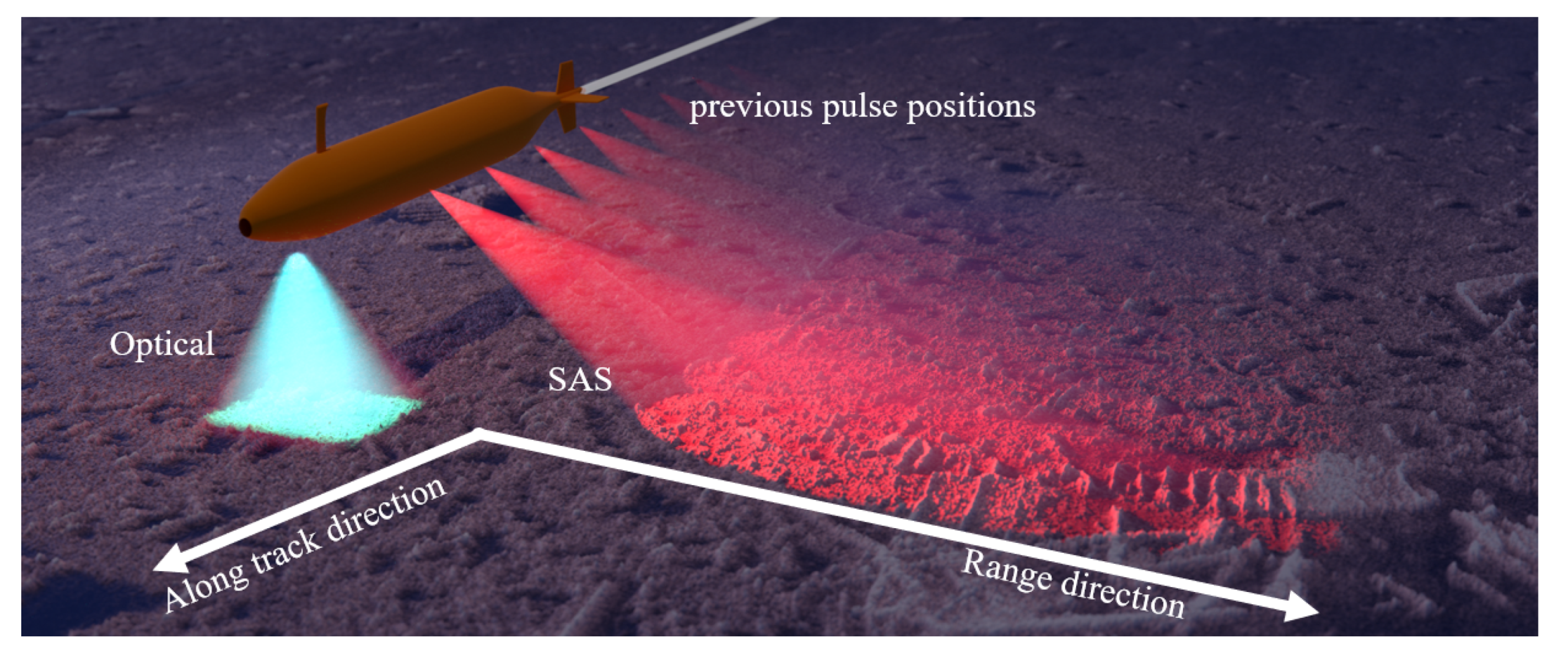
The optical sensor used was a Tilefish downward-looking camera with a 400 W strobe LED array [
9]. The 10.7 megapixel camera captures small details, imaging the seafloor as a perspective projection of the 3D environment at 1 mm resolution [
10]. However, the coverage rate is limited by a downward-looking geometry with a short stand-off, a result of the strong attenuation of electromagnetic waves in water (shown in
Figure 2). For a typical AUV altitude of 6 m and speed of 2 m/s, the area coverage rate becomes 12 m
/s, or 0.043 km
/h [
9]. At depth, a colocated illumination source is necessary; this arrangement does not produce a significant shadow when looking at proud objects. Additionally, sediment deposited on sunken objects produces reflectivity similar to that of the seafloor, leading to low-contrast images.
The other primary sensor used on the HUGIN vehicle was a HISAS synthetic aperture sonar with a centre frequency of 100 kHz and a 30 kHz bandwidth [
11]. Active sonar emits an acoustic signal and infers information about the environment from the time delay and intensity of the echo [
3]. Sonar resolution is limited by its aperture size; to improve resolution synthetic aperture sonar (SAS) is a technique for generating a large aperture on a moving vehicle. In this study, the FOCUS software developed by FFI was used to process the raw data (see [
12] for more details on the SAS processing pipeline for the HUGIN AUV). The output typically used for target recognition, and indeed used in this study, is an intensity image where pixel values correspond to echo strength. It is an orthographic projection of the 3D space which has an aerial-photograph-like quality [
3].
Good acoustic propagation in water permits a large effective range of 200 m per side (at 2 m/s vehicle speed) and hence a greater instantaneous coverage rate: 2.88 km
/h at 4 cm resolution [
9]. The divergence of acoustic signal means that objects at a greater distance are ensonified by more pings. The synthetic array can therefore be longer, allowing range-independent resolution. SAS is typically operated at a shallow grazing angle, resulting in a strong reflection and shadow, highlighting proud objects (
Figure 2). Furthermore, the high density of metallic objects (e.g., UXOs) returns a strong acoustic echo, giving a good contrast to background sediment. The major drawback is limited resolution; this means small targets have poor detail, being represented by only a few pixels.
3. Labelling Methodology
The lack of ground truth in the survey area creates a need for a labelling method that incorporates uncertainty. To this end, we have used an ordinal labelling scheme, whereby each detected object is assigned one or more classes arranged in order of likelihood by the human labeller. A ranked list is a more natural and consistent process for a human labeller compared to assigning numeric values (e.g., probabilities) [
13,
14]. Various schemes exist for capturing object location (e.g., centre of object, bounding box, oriented bounding box, pixel mask) [
15]. However, we chose to use rectangular boxes as a trade-off between precision and labelling efficiency. Note that there are automatic approaches that refine the imprecise boundaries, e.g., GrabCut [
16], making labelling pixel-precise boundaries hard to justify. The entire Skagerrak survey area is 450 km
, but only 0.1 km
of it was labelled, taking 35 h (more details are provided in
Section 4). A single person (the lead author) performed the labelling of the multi-sensor data, via a custom-made user interface.
The labelling process was initiated on a SAS image. The image was methodically scanned, and all observed objects were bounded by a rectangular box. Each of these objects was assigned a ranked list of likely classes. The available classes are as follows and were selected based on prior knowledge of the expected chemical munition types at the dumpsite [
1]:
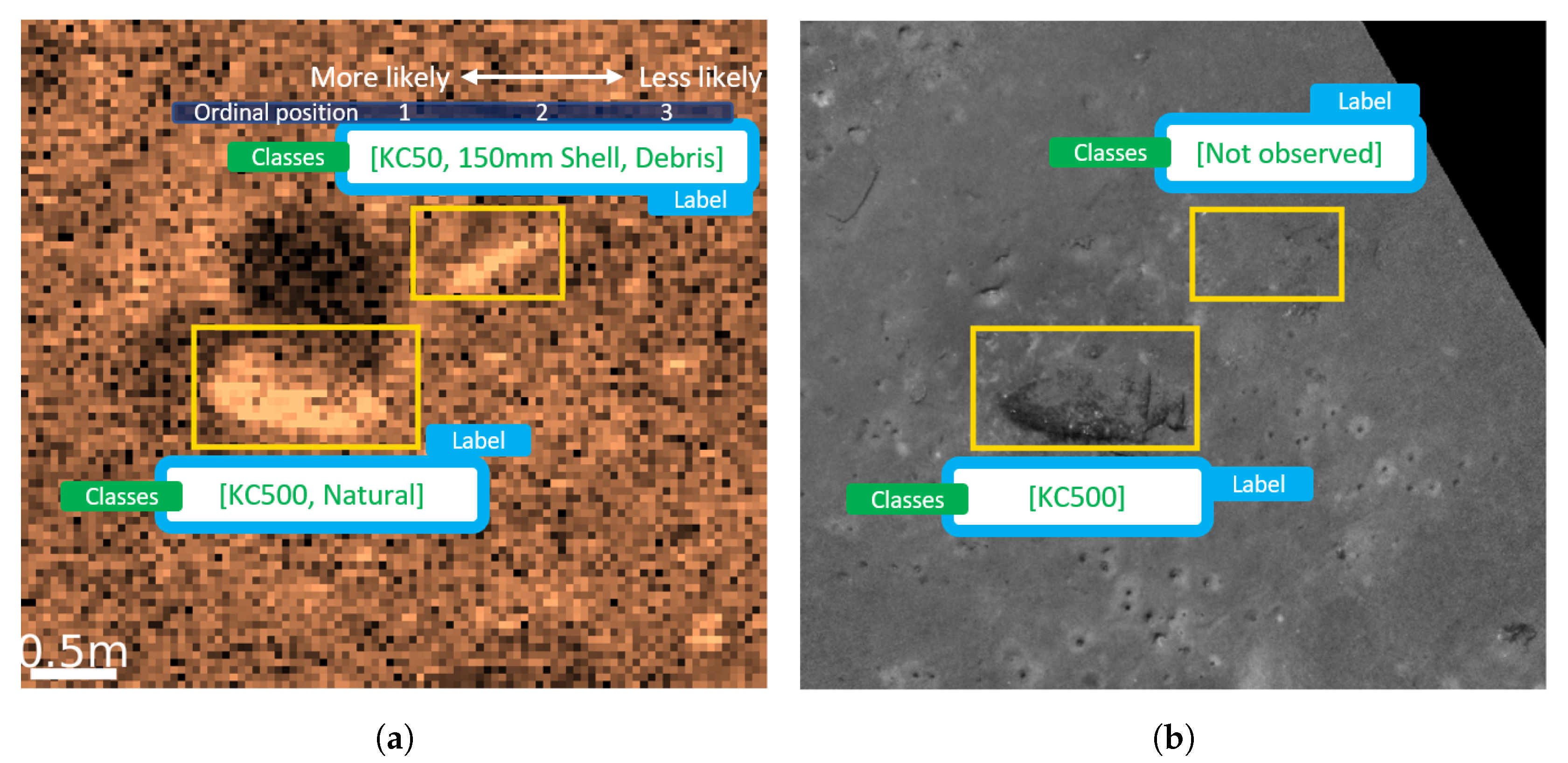
The initial labelled SAS image was used to define a common coordinate system in which all subsequent images were referenced. The bounding boxes from this previously labelled image are then overlaid onto overlapping images for independent relabelling in the different views, e.g., the optical image shown in
Figure 3b. A bounding box from an alternative view or modality may not contain an observable object. Therefore, a “not observed” label was required for these cases. Any additional objects detected would also be bounded and a second pass performed on previously labelled images to label any missed objects.
Examples of two detected and labelled objects from a SAS image are given in
Figure 3a. In one case, the object has been labelled as a likely 500 kg bomb, but with uncertainty due to its resemblance to a bolder (natural). In the other case, the object has been labelled with less certainty, due to its size and shape being similar to a 50 kg bomb, a 150 mm shell, and possibly debris due to its high aspect ratio. In this case, greater detail from an overlapping optical image (
Figure 3b) allowed the larger object to be labelled as a 500 kg bomb, with no feasible alternatives: high certainty. The other object, however, was not visible in the optical image so is labelled “not observed”.
While the relabelling from different views was performed independently, the bounding box size may influence the human labeller because the size and aspect ratio implies specific UXO types. In the case of piled objects, the distinction between individual objects is not always clear, and segmentation of amorphous regions may be more suitable than the counting of individual UXOs in these areas. In summary, the probability of an object belonging to a class is some unknown function of the class’s rank (position in the ordinal list) and the length of the list. Rank reciprocal (inverse) [
17], rank sum (linear) [
17], and rank ordered centroid [
18] are some common mappings used in multicriteria decision-making. These are consistent with our ability to rank classes. However, without a method for validating the choice of mapping the simplest regime, rank sum is recommended. The multi-class, multi-view modality labels do, however, provide a rich source of information that is representative of the precision of a human labeller.
4. Results
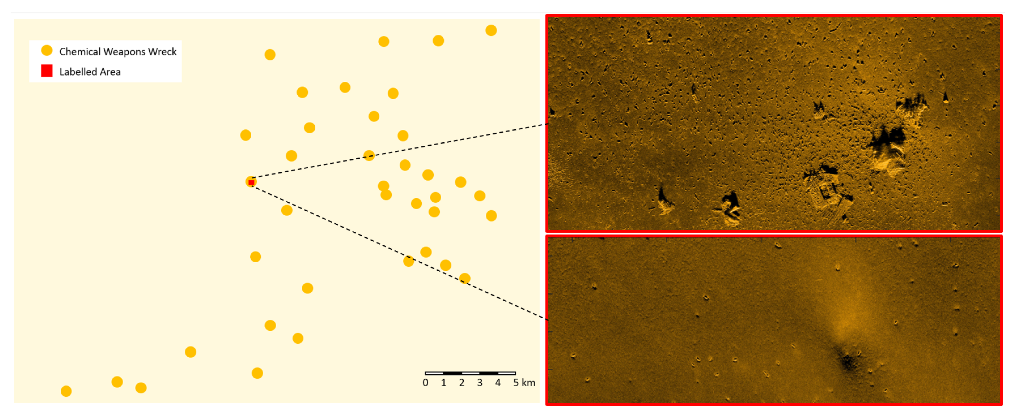
The labelled dataset covers an area of 0.1 km
; this is only 0.02% of the total 450 km
surveyed area shown in
Figure 4. However, we chose the area as it is representative of many challenging scenarios: piled objects, a variety of debris types, and sparse and dense regions. The 0.1 km
labelled area resulted in 8920 labels of 5331 objects. A single user was able to average one label every 14.2 s, taking 35 h total. Taking a “worst-case” area for labelling, as we have done, is a compromise for generating representative datasets with limited labelling resources.
The labels themselves consist of multiple classes. In
Figure 5, we calculate the ratio of labels containing different combinations of classes in addition to the distribution of classes. This analysis revealed that the labeller frequently could not differentiate between objects of similar size. The labeller also found it challenging to distinguish debris, a result of debris having no expected size or shape. Historic UXOs are exposed to a corrosive environment for potentially many decades. This results in decay, biofouling, and partial or full burial, further impeding human labelling. Grouping debris and natural objects would alleviate a frequently confused pair; however, debris is useful to classify as it indicates the presence of UXOs nearby. Grouping classes of similar objects, however, is a sensible conclusion from this result, which we investigate later.
Munition types are manufactured and disposed of in varying quantities, therefore, a labelled dataset reproduces this imbalance.
Figure 5b quantifies the imbalance in the Skagerrak UXO dataset with many more cases of small munitions (shells) than larger munitions (bombs). However, the number of dangerous and harmless objects is more balanced. The Imbalance between classes is a necessary consideration for the application of machine learning to avoid bias towards overrepresented classes. Practical solutions involve balancing the distribution (data-level), modifying the learning algorithm to alleviate bias (algorithm-level), or a combination of both (hybrid method) [
19].
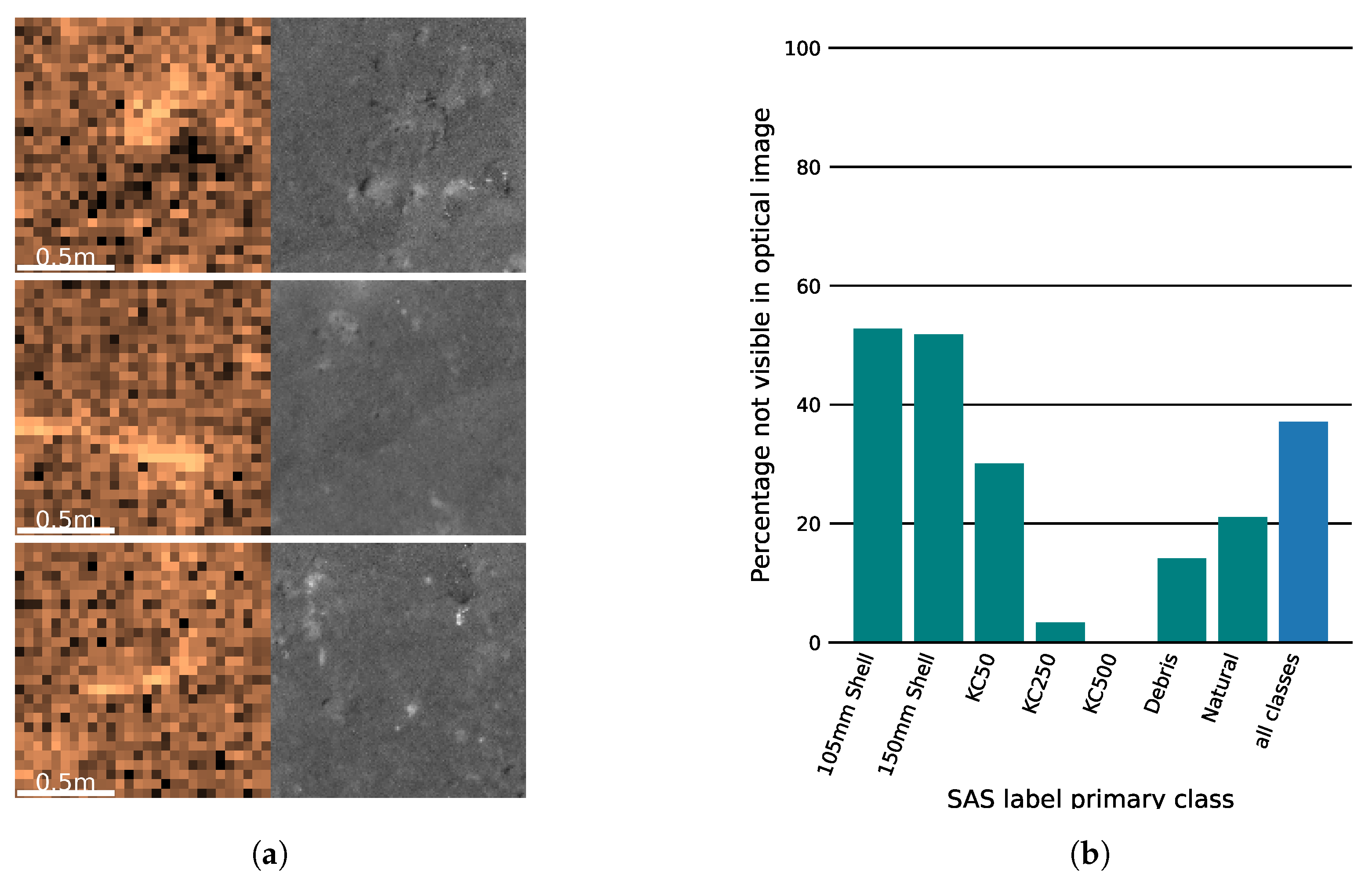
At 100 kHz, the HISAS is capable of some penetration of sediment [
2], allowing shallowly buried objects to be detected. We presupposed that the “not observed” labels for optical images correspond to buried objects. We quantify the extent of suspected burial in
Figure 6 alongside examples of SAS images with their optical image counterparts taken from Skagerrak. We observed that small dense objects (shells) are more frequently buried compared to larger objects (bombs). The high proportion of buried objects is surprising, as optical images are commonly considered as providing a means of validating SAS classifications [
9].
The comparison between image modalities can also be made between multiple SAS views of the same objects. In
Figure 7, we quantify the impact of the SAS look direction on object visibility, alongside some examples from the Skagerrak dataset. From
Figure 7a, we observed that the visibility of an object’s highlight and shadow can depend on its orientation. In certain cases, an object can be near-invisible from an alternative SAS look direction, and our labels show that this is more likely for smaller objects.
One challenge we have identified, but are not able to quantify, is target variability: various states of assembly and decay reduce the clarity for a labeller. Instead, we quantify label accuracy, which is a consequence of target variability combined with the other challenges discussed previously. The best optical labels were identified from having only a single class assignment. The detail visible in optical images permits high confidence in these labels, which are used as pseudo ground truth.
Figure 8 shows the result of assessing SAS labels against this pseudo ground truth.
Both class position and label length correlate negatively with accuracy, and this validates our use of ordinal lists for likely classes. However, 60% accuracy for the best SAS labels (green) limits the feasability of applying supervised learning (for a comprehensive review of methods robust to noisy labels, see [
20]). Furthermore, of the 5331 objects from SAS images, only 585 have optical overlap. This is generally the case due to a much slower coverage rate of 0.043 km
/h for optical images compared with 2.88 km
/h for SAS (see
Section 2 for more details). Additionally, only 290 of the 585 optical images provide “pseudo ground truth” as many are obscured by partial burial and degradation. This is an insufficient number for typical supervised learning approaches [
21]. The accuracy can, however, be improved by grouping into fewer classes. Using only two very broad classes of harmless versus dangerous yields an improvement in accuracy from 60% to over 80%. Separating instead into similar-sized UXOs (bombs, shells, debris, and harmless) does not significantly reduce this improvement, and provides a good trade-off for discrimination versus accuracy.
5. Conclusions
We have defined a methodology for labelling multi-modal and multi-view images of objects on the seafloor. The methodology is intended for applications where ground truth information is unavailable, for example, at historic UXO dumpsites. It has been demonstrated on multi-view SAS and optical survey data collected from the Skagerrak chemical munitions dumpsite in Norway, where the target objects are bombs and shells amidst a field of debris and natural clutter.
A counterintuitive finding in this study was the revelation that the optical survey data do not provide sufficient ground truth of the chemical munitions dumpsite at Skagerrak for adequately labelling the objects. This is because a significant proportion of objects are buried and these are visible in the acoustic images and not the optical images. The low accuracy of labels (particularly for SAS data) and a small number of optical “pseudo ground truth” labels motivate future research into self-supervised learning [
22]. This is where a small amount of labelled data is used to bootstrap learning from a large amount of unlabelled data.
Using only optical labels with high confidence as pseudo ground truth (i.e., non-buried objects only), we quantified accuracy for the three class assignment schemes: (1) unique classes for specific UXOs (e.g., 500 kg bomb, 250 kg bomb, etc.); (2) simplified groupings of UXOs (e.g., bombs, shells, debris, and natural); and (3) a binary dangerous versus harmless label. We concluded from this work that the simplified grouping (shells, bombs, debris, and natural) gave the best trade-off between accuracy and discrimination: −60% for seven classes versus 80% for four classes.


 ,
, 