Article

Monitoring the Ice Thickness in High-Order Rivers on the Tibetan Plateau with Dual-Polarized C-Band Synthetic Aperture Radar

1
Northwest Institute of Eco-Environment and Resources, Chinese Academy of Sciences, Lanzhou 730000, China
2
University of Chinese Academy of Sciences, Beijing 100049, China
3
Key Laboratory of Remote Sensing of Gansu Province, Heihe Remote Sensing Experimental Research Station, Chinese Academy of Sciences, Lanzhou 730000, China
4
College of Geography and Environmental Science, Northwest Normal University, Lanzhou 730070, China
*
Author to whom correspondence should be addressed.
Remote Sens. 2022, 14(11), 2591; https://doi.org/10.3390/rs14112591
Submission received: 27 March 2022 / Revised: 8 May 2022 / Accepted: 25 May 2022 / Published: 27 May 2022
(This article belongs to the Special Issue Remote Sensing in Snow and Glacier Hydrology)

Abstract

:
River ice on the Tibetan Plateau has important impacts on the ecosystem and hydrology. High-resolution Synthetic Aperture Radar (SAR) is an important tool for monitoring the thickness of river ice in high-altitude areas without ground data. However, due to the complex topography and narrow width, it remains challenging to monitor the ice thickness of high-order rivers (high-level branches in the plateau river system) on the Tibetan Plateau using SAR. Therefore, this paper focuses on inverting the ice thickness by utilizing dual-polarized C-band radar data. We select a typical watershed in the northeastern Tibetan Plateau, namely, the Babao River basin (including the Babao River and Binggou River), as the study area. The results show the following: (1) Dual-polarized C-band radar data have the potential to monitor the ice thickness of high-order rivers. The RMSEs of the Babao and Binggou Rivers are 0.109 m and 0.258 m, respectively. (2) Ascending and descending orbit radar images perform differently in retrieving the ice thicknesses of rivers with different directions. (3) The thickness of river ice affects the inversion accuracy. (4) Polarization parameters have varying explanatory capacities depending on the river characteristics. Our findings can provide a reference for the subsequent development of highly generalizable river ice inversion equations using dual-polarized radar data.

1. Introduction

Monitoring river ice in cold regions is important for water resources management, flood monitoring, transportation, and hydraulic modeling [1,2]. Current research on river ice covers the main issues of freezing and breakup [1,3,4,5], extent [2,5,6], type [7,8], and thickness [9,10]. However, these investigations mainly evaluated rivers such as the Saint-François River [10] and the Mackenzie River [11] in Canada, whereas the Tibetan Plateau, known as the “Water Tower of Asia”, remains largely unexplored in this regard. Nevertheless, due to its complex topography, long winter ice season, and extensive distribution of river ice, the Tibetan Plateau is one of the most sensitive regions to global climate change worldwide [6,12]. The extent and thickness of river ice greatly affect the hydrological processes atop the plateau.
River ice thickness, which is the most difficult variable to measure in the whole field of river ice research, can be estimated empirically based on regional environmental and meteorological data [10]. For example, Li et al. [13] used hydrometeorological data to obtain a statistical relationship for the thickness of river ice in the main stream of the Songhua River. Barzegar et al. [11] used machine learning methods to estimate river ice thickness in terms of snow depth and average air temperature. Unfortunately, these non-remote sensing empirical methods are limited by the conditions under which the input data are acquired, are more difficult to implement in areas lacking ground data, and are highly empirical in nature.
Alternatively, because of its high resolution, weather independence, and sensitivity to the structure, surface, and thickness of ice [14,15], synthetic aperture radar (SAR) has considerable potential in monitoring ice thickness [10,16,17]. Lindenschmidt et al. [16] used C-band RADARSAT-2 to explore the relationship between ice thickness and horizontal–horizontal (HH) polarization and demonstrated both that the information obtained by RADARSAT can be used in empirical equations and that the radar images are correlated with the mean ice thickness of each section. Toyota et al. [18] used HH-polarized L-band data from the Advanced Land Observing Satellite (ALOS) Phased Array L-band Synthetic Aperture Radar (PALSAR) to establish a regression equation for sea ice thickness, indicating that SAR data are a promising avenue for determining the ice thickness distribution. Mermoz et al. [10] proposed a method to invert river ice thickness using HH-polarized RADARSAT-2 C-band data and obtained the spatial distribution of river ice thickness. Sanden and Drouin [19] used RADARSAT-2 (C-band) and ALOS PALSAR (L-band) backscatters to relate the type and thickness of river ice and discussed the effect of the microwave wavelength on the inversion accuracy, showing that C-band RADARSAT data are better than L-band ALOS PALSAR data. For some types of river ice, backscattering can accurately predict the river ice thickness. In general, considering the current microwave methods for inverting the thickness of river ice, fully or dual-polarized methods with C-band data are consistently regarded as capable of obtaining relatively reliable results.
As mentioned above, studies on the microwave inversion of river ice have focused on large Arctic rivers with wide (approximately 400 m to 3 km) streams [10]. However, river ice on the Tibetan Plateau is distributed mainly in the upper reaches of high-altitude mountainous watersheds with complex topography, namely, on high-order rivers with relatively narrow widths of approximately 35–126 m and an average river width of 91 m [20]. Moreover, many factors, such as mountain shadows and topography, affect the inversion of river ice thickness, and measured data are scarce. These unfavorable factors greatly complicate the microwave inversion of river ice on the Tibetan Plateau. Consequently, relatively few studies have been performed on either the phenology or the extent of river ice atop the Tibetan Plateau (only Yang et al. [21] and Li et al. [2,6] have studied the extent of river ice on the Tibetan Plateau), and thus, work on the inversion of river ice thickness is severely lacking.
In general, microwave methods are the most promising remote sensing tool for the inversion of river ice thickness. However, whether such methods are effective for high-order rivers in such a complex region as the Tibetan Plateau remains unclear, and the effects of different altitudes, river widths, and river ice thicknesses on the inversion accuracy are poorly understood. Therefore, to fill the gap in the research on river ice thickness on the Tibetan Plateau, we use dual-polarized C-band Sentinel-1 data to explore a microwave method for inverting river ice thicknesses on the Tibetan Plateau. Furthermore, we evaluate the accuracy of microwave-inverted river ice under different development states and in different regions with complex topographies.

2. Study Site and Datasets

2.1. Study Site

The study area is a typical watershed in the northeastern part of the Tibetan Plateau, namely, the Babao River basin (including the main stream of the Babao River and the tributaries of the Binggou River) (Figure 1). The width of the Babao River is approximately 50–1000 m, the elevation is approximately 2800–3300 m, and the topography is relatively flat with a northwest–southeast orientation; in contrast, the width of the Binggou River is approximately 20–200 m, the elevation is approximately 3300–4000 m, and the topography is relatively complex with a north–south orientation.
The Babao River is 104.1 km long, while the Binggou River is 23.5 km long and converges into the Babao River. River ice in the Babao River basin starts to grow in October, reaches its peak in February, and gradually decreases in May, reaching a maximum ice area of 52.93 km2; the distribution of river ice is discontinuous and is related to the shape, slope, and temperature of the river [6]. The Babao River basin contains a large amount of seasonal permafrost and perennial permafrost and is considered to be representative of the cold regions atop the Tibetan Plateau. The basin has an average daily flow of 14.5 m3/s, an average annual flow of 4.59 × 10⁸ m3, an average elevation of 3604 m, average annual precipitation of approximately 400 mm, an average annual temperature of approximately 0.7 °C, frequent snowfall, a multiyear snow cover of 0.48%, and a seasonal snow cover of 17.53%. When the rivers in this study area freeze in winter, most of the river ice is covered by a thin layer of snow.

2.2. Field Sampling Data

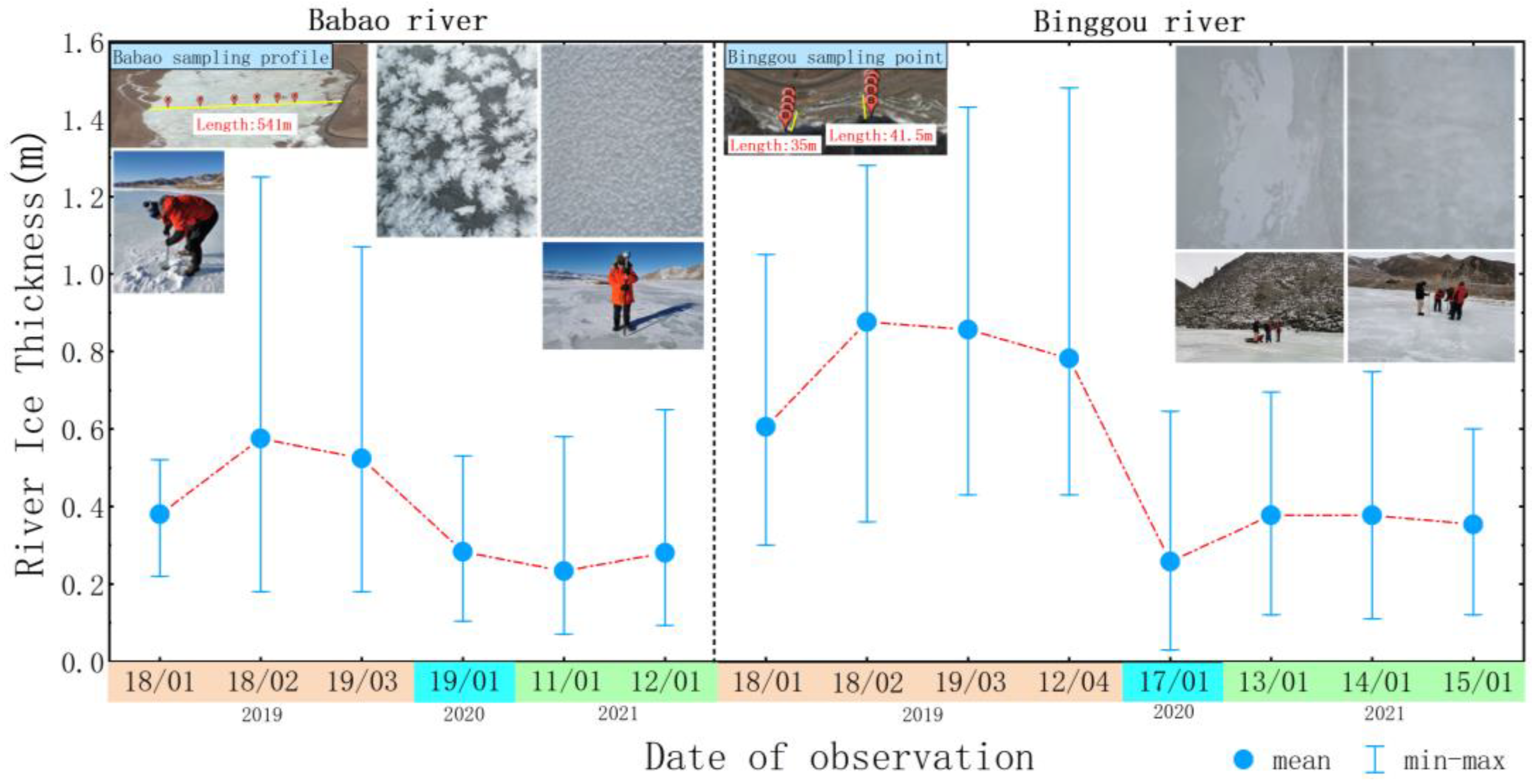
Field data were obtained on 18 January, 18 February, 19 March, and 12 April 2019, 17 January 2020, and 11 January through 15 January 2021 (11 to 12 January on the Babao River and 13 to 15 January on the Binggou River) (Figure 2 and Figure 3).
The river ice thickness sampling points were located using a handheld GPS in 2019–2020 and a GPS real-time kinematic (RTK) device in 2021, with positioning errors at the centimeter level. The Babao River data were collected along a profile, while the Binggou River data were randomly sampled along the river. The measured data were collected by using an ice chipping tool, and tape measures were utilized to measure the ice thickness at that time. A total of 112 samples were collected from the Babao River, and 153 samples were collected from the Binggou River. In considering the two river data collection methods, radar image resolution, shading, and other factors, the measured data from the Babao River were simulated by profile averaging, while those from the Binggou River were simulated using individual points. Figure 2 shows the measured data after profile averaging and the states, locations, sampling methods, and distributions of the measurement points of river ice. The average river ice thickness of the Babao River in January is approximately 0.30 m, while in February and March, it is approximately 0.54 m; in April, the ice has basically melted. The average thickness of river ice in the Binggou River is approximately 0.45 m in January; afterward, the river ice thickness reaches 0.85 m on average in February into March and starts to thin out in April (at approximately 0.70 m) before essentially melting in May.

2.3. Remote Sensing Data

In this study, single look complex (SLC) and ground range detected (GRD) dual-polarized (VV-VH) Sentinel-1 satellite data in interferometric wide swath (IW) mode were used, and the incidence angles of the acquired images ranged between 30° and 45°. The data are shown in Figure 3.
The Sentinel-1 series of satellites, which are managed by the European Space Agency (ESA), consist of two satellite constellations, A and B. These satellites are equipped with C-band SAR sensors and feature a revisit period of 6 days with four modes of data acquisition: strip map (SM) mode, extra wide swath (EW) mode, IW mode, and wave (WV) mode. The study area is covered by only the IW mode, which has the advantages of a high spatial resolution (5 m × 20 m) and broad coverage (250 km). The product levels available for download are Level-0 raw data and Level-1 SLC and GRD data.

3. Methods

The main method used in this study inverts the river ice thickness by establishing a linear or nonlinear regression equation (Equation (1)) and a stepwise regression equation (Equation (2)) between the polarization parameters of Sentinel-1 and the measured ice thickness. By inverting the river ice thickness, we explore the answers to the following questions: (1) Are there inversion formulas to invert the thickness of river ice in high-order rivers? (2) How accurate and applicable are these inversion formulas in high-altitude mountainous areas with complex topography? (3) How do the river ice conditions, river size, and topography affect the inversion accuracy?
y = f ( x )
y = β 0 + β x 1 + β x 2 + + β n x n
For this simulation, linear, quadratic, cubic, compound, logarithmic, exponential, inverse, and power functions are chosen for f(x) in Equation (1). The dependent variable y is the measured river ice thickness, and the independent variable x is a certain polarization parameter of Sentinel-1.
The main principle of the stepwise regression in Equation (2) is to introduce the independent variables into the equation one by one, and each introduced variable is subjected to F and t tests; when the tests for these independent variables become nonsignificant due to the introduction of another independent variable, the most recent introduced variable is removed. In Equation (2), y is the explained variable, β1βn denote the regression coefficients, β0 is the constant model fit, and x1xn are the explanatory variables. Pearson’s coefficient of determination, R2, is used to measure the fit, and the fitted equation with the highest R2 is retained to invert the river ice thickness.
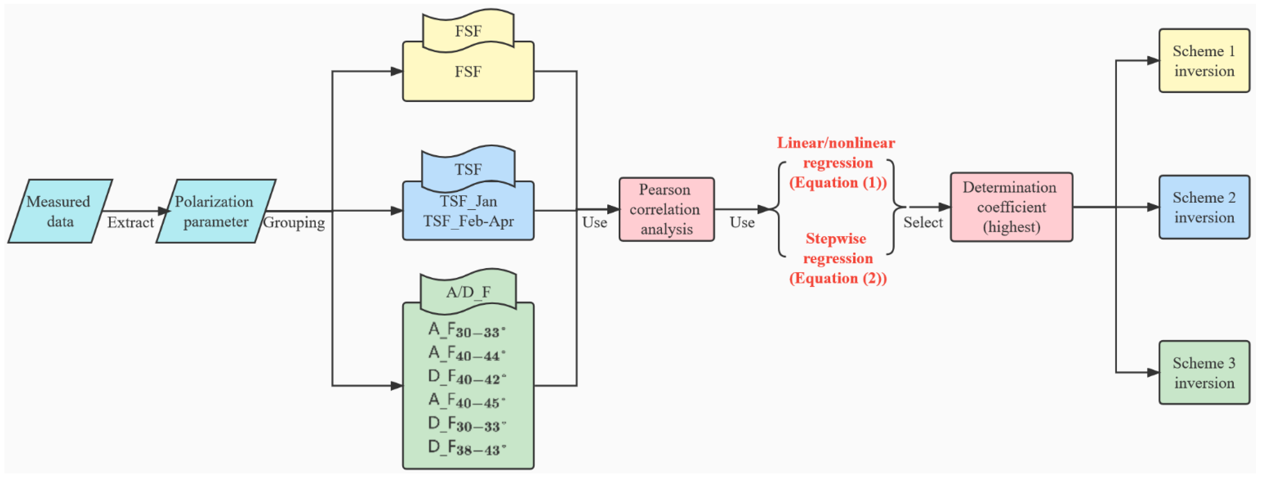
The river ice thickness and the image orbit could heavily influence the inversion accuracy. To clear these influences, we set three inversion schemes based on the measured data and polarization parameters:
Scheme 1: Full sample fitting (FSF) is to determine the effectiveness of microwave inversion of river ice thickness in this region.
Scheme 2: Time segment fitting (TSF) mainly determines whether the inversion formulas obtained at different periods can invert river ice of different thicknesses.
Scheme 3: Radar ascending or descending fitting (A/D_F) explores how radar images on ascending and descending orbits affect the river ice thickness inversion. The acquired radar images are classified and fitted by different ascending and descending orbits and incidence angles.
The program framework is as follows (Figure 4).

3.1. Sentinel-1 Polarization Parameter Acquisition

Sentinel-1 images are subjected to an orbit correction, a radiometric calibration, debursting, polarization filtering, and a terrain correction. In this study, the Refined Lee filter is chosen to remove speckle noise from the SAR images and to solve the noise filtering problem of the subdiagonal elements of the polarization covariance matrix, which is neither a multiplicative nor an additive model [22]. Shuttle Radar Topography Mission (SRTM) data with a resolution of 30 m are utilized for the Range-Doppler terrain correction [23].
To obtain the polarization parameters, namely, the entropy (H), scattering angle (α), and anisotropy (A), this paper mainly employs Hα dual-polarization decomposition. Initially, polarization decomposition was designed for fully polarized data (RADARSAT) [24], whereas Sentinel-1 data provide only dual-polarized information, so the extraction method needs to be modified. The concept of polarization decomposition is based on the complex scattering matrix [S] (where Sfull indicates a fully polarized scattering matrix and Sdual indicates a dual-polarized scattering matrix), and for Sentinel-1, a correction needs to be applied to the expression of its scattering vector [25,26], that is, to transform Sfull into Sdual (Equations (3) and (4)):
S f u l l = ( S H H S H V S V H S V V )
S d u a l = ( 0 0 S V H S V V )
where Sfull and Sdual denote the backscattering coefficient matrices of fully and dually polarized image elements, respectively, SHV denotes the backscattering coefficient of H-polarized transmission and V-polarized reception, SVH denotes the backscattering coefficient of V-polarized transmission and H-polarized reception, SHH denotes the backscattering coefficient of H-polarized transmission and H-polarized reception, and SVV denotes the backscattering coefficient of V-polarized transmission and V-polarized reception.
Then, Equations (3) and (4) are expressed as scattering vectors, and the outer product is obtained with their conjugate transpose to obtain the covariance matrix and coherence matrix (describing the scattering process). The eigenvalues and eigenvectors are extracted, and the entropy, scattering angle, and anisotropy are calculated.
H = i = 1 n P i log n P i
P i = λ i j = 1 n λ j
Entropy is a measure of the randomness of the scattering process and takes values within the range 0–1. Entropy is calculated using the logarithm of the eigenvalues of the coherence matrix (Equations (5) and (6)), where Pi refers to the probability of the contribution of each eigenvalue and λ refers to the eigenvalue of the covariance matrix. n is assumed to be three under full polarization and two under dual polarization.
Anisotropy is the complement of the entropy and represents the relative strength of the first and second scattering mechanisms. Anisotropy is calculated using the second and third eigenvalues of the covariance matrix under full polarization (Anisotropyfull or Afull for short) and the first and second eigenvalues of the covariance matrix under dual polarization (Anisotropydual or Adual for short) (Equations (7) and (8)).
A f u l l = λ 2 λ 3 λ 2 + λ 3
A d u a l = λ 1 λ 2 λ 1 + λ 2
α, the scattering angle, describes the main scattering mechanism (Equations (9) and (10)). An α angle close to 0° indicates surface scattering, while a value close to 45° indicates volume scattering, and a value close to 90° indicates dihedral angle scattering.
α = i = 1 n P i α i
α i = cos 1 ( | v 1 i | )
In the above equations, αi is the alpha angle, v is the eigenvector, and α is defined as the average of the scattering angles of the eigenvector v.
Finally, the acquired polarization parameters are resampled to a spatial resolution of 10 m.

3.2. River Ice Extent

This study employs the river ice extent data published by Li et al. [2]. These data were extracted by Google Earth Engine (GEE) to determine the maximum river ice extent of the Babao River, and the algorithm was validated to be reliable on the Tibetan Plateau with an average overall accuracy of 99.9% and an average kappa coefficient of 0.96.

3.3. Program Design

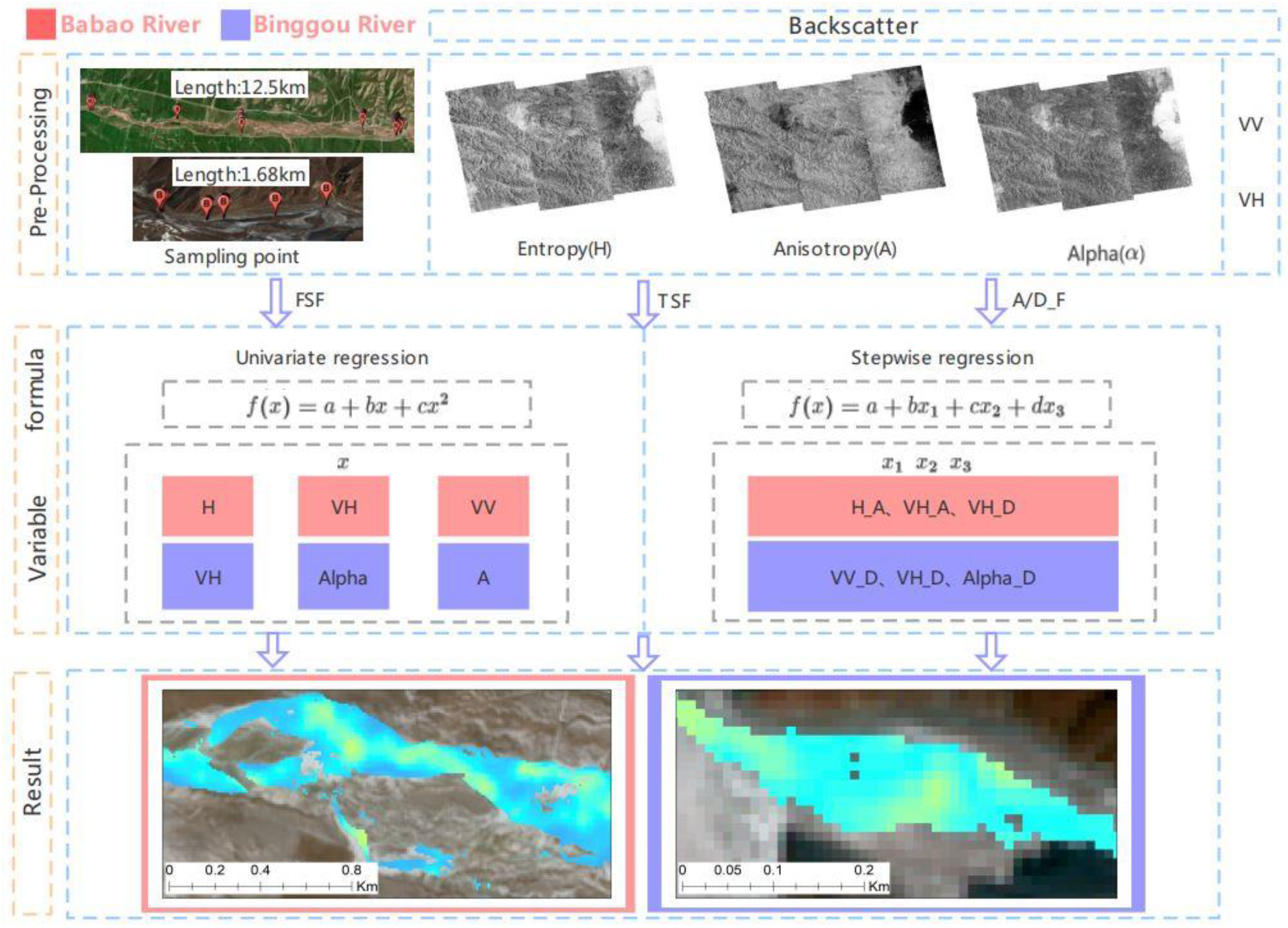
In considering the responses of the polarization parameters to different river ice development states and surrounding terrain conditions, the fitting was divided into three schemes according to the month, elevation, and complexity of the terrain. Spatially, the Babao River is less influenced by the surrounding mountains and has a wide channel; in contrast, the Binggou River is a high-order river with a narrow channel, and the surrounding mountains exhibit a large elevation difference. Therefore, these two regions are considered separately. The framework for implementing is shown in Figure 5.
Scheme 1: FSF uses all the measured data for the simulation to validate the microwave method for inverting the river ice thickness in the region using leave-one-out cross-validation (LOOCV). This scheme relates the measured data to the radar polarization parameters and trains the best-fitting equation by Equations (1) and (2) while considering all river ice development states.
Scheme 2: TSF analyzes whether the accuracy of the inversion formula changes under different river ice development conditions and whether the inversion formulas obtained at different time periods have the ability to invert river ice of different thicknesses. In this study, the TSF scheme is divided into two fitting equations according to the different development statuses of river ice at different times, namely, fitting the measured data in January (TSF_Jan) and fitting the measured data in February through April (TSF_Feb–Apr). River ice accumulates in January and therefore is relatively thin and experiences less ablation; from February to April, river ice is fully developed. This scheme is validated mainly using LOOCV and independent validation.
Scheme 3: A/D_F explores whether radar images on ascending and descending orbits have an effect on the river ice thickness inversion. The acquired radar images are classified and fitted by different ascending and descending orbits and incidence angles. The Babao River images are divided into ascending orbit 30–33° (ascending radar images with incidence angles of 30–33°, abbreviated as A_F30–33°), ascending orbit 40–44° (ascending radar images with incidence angles of 40–44°, abbreviated as A_F40–44°), and descending orbit 40–42° (descending radar images with incidence angles of 40–42°, abbreviated as D_F40–42°). The Binggou River images are similarly divided into ascending orbit 40–45° (A_F40–45°), descending orbit 30–33° (D_F30–33°), and descending orbit 38–43° (D_F38–43°).
In addition to the above three schemes, this paper also applies two river ice inversion schemes of different levels to each other: the inversion schemes of the Babao River are used for the Binggou River, and the inversion schemes of the Binggou River are used for the Babao River. In this way, the applicability of the inversion schemes is investigated for the same complex terrain but on different river levels.
The independent variables were selected by correlation analysis and the model R2 values for each scheme. When the variance inflation factor (VIF) of the independent variable was greater than 10 (Equation (11)), the simulation was not considered using multiple regression, and only the independent variable with the highest correlation was used for linear or nonlinear regression fitting (see Figure 6 and Figure 7 for the fitting results).
The VIF was used to measure the severity of collinearity in the multiple regression model, and R i 2 denotes the R2 of the linear regression model of the independent variable xi on the remaining independent variables in the model. VIF < 10 indicates no collinearity among the independent variables, whereas VIF > 10 indicates severe multicollinearity in the regression model.
V I F = 1 1 R i 2

3.4. Evaluation Methods

In this study, the results were validated using LOOCV and the independent validation approach. The LOOCV method is used to evaluate the accuracy of the river ice thickness simulation, in which one data point is removed from the measured data in each simulation, and the simulated value of the removed data point is obtained by regression or simulation. Then, the simulated value is compared with the measured value, and an error is calculated. Then, the measured data point is placed back into the dataset, a different measured data point is removed, and the same method is applied to obtain the corresponding simulated value. The above process is repeated until all the measured data are estimated, and the root mean square error (RMSE) between these measured and simulated values is calculated, where the calculated RMSE is abbreviated as L_RMSE.
The independent validation approach, on the other hand, uses a portion of the measured data for simulation and the remaining portion for validation. That is, the RMSE is calculated using the measured values that are not involved in the fitting equations in comparison with the values simulated by the fitting equations. The RMSE calculated here is abbreviated as I_RMSE.
In addition, the following metrics were used to evaluate the fitting equations.
(1) The correlation coefficient (R) is used to study the degree of linear correlation between variables: values of 0.8–1.0 indicate a very strong correlation, 0.6–0.8 indicate a strong correlation, 0.4–0.6 indicate a moderate correlation, 0.2–0.4 indicate a weak correlation, and 0.0–0.2 indicate a very weak correlation or no correlation.
(2) The coefficient of determination (R2), also known as the goodness of fit, is used to evaluate the quality of fit. The value ranges between 0 and 1. In the following formula, y ^ i denotes the fitted value, y i   denotes the observed value, and y ¯ i indicates the mean of the observed values.
R 2 = ( y ^ i y ¯ i ) 2 ( y i y ¯ i ) 2
(3) The root mean square error (RMSE) is a measure of the regression equation error, where n is the number of observations, y ^ i is the fitted value, and y i   is the observed value.
RMSE = i = 1 n ( y ^ i y i ) 2 n

4. Results

4.1. Babao River

4.1.1. Scheme Fitting Effects

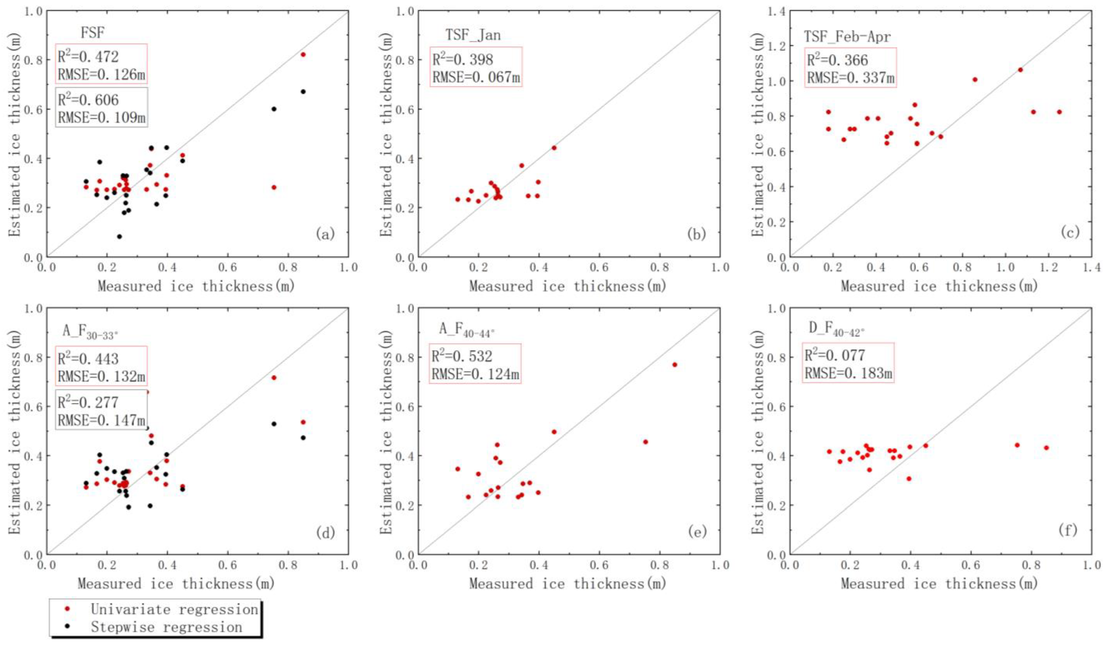
When using the FSF scheme, the polarization parameter with the strongest correlation is H, with an R2 of 0.472 and an L_RMSE accuracy of 0.156 m (Figure 6). When using the stepwise regression method for the simulation (Figure 7), the optimal parameters chosen for the scheme are H and VH polarization, with an R2 of 0.606.
When using the TSF scheme, the January fitted equation (TSF_Jan), although featuring a weakly moderate correlation (−0.408), has a simulated L_RMSE of up to 0.079 m. In contrast, the fitted equation for February through April (TSF_Feb-Apr) is significantly correlated with the VH polarization mode, but the L_RMSE reaches 0.267 m. The VIFs of all independent variables are greater than 10 in this scheme when stepwise regression analysis is performed, indicating serious multicollinearity, so stepwise regression was not employed with this scheme.
When using the A/D_F scheme, the ascending orbits (A_F30–33°, A_F40–44°) are more suitable for inverting the ice thickness in the Babao River, with an L_RMSE of 0.160 m (A_F30–33°), second only to the FSF scheme with an RMSE of 0.156 m. The accuracy of the descending orbit (D_F40–42°) is poorer than that of the ascending orbits, with an L_RMSE of 0.197 m.
Except that the estimated values of TSF_Feb–Apr and D_F40–42° are relatively discrete, the rest of the fitting equations can be better close to the 1:1 line (Figure 8). When the measured value is smaller, the linear or nonlinear regression value of TSF_Jan and FSF is closer to the 1:1 line. In addition, the equation fitted by the ascending orbit data is closer to the 1:1 line than the one fitted by the descending orbit data.
Overall, the FSF, TSF_Jan, and A_F30–33° fitting equations are most suitable for inverting the ice thickness in the Babao River, and the ascending orbit radar images are better than the descending orbit radar images. This indicates that the river ice development status, ascending and descending orbits of radar images, and incidence angle influence the inversion outcome. Moreover, the simulation accuracy is improved when multiple variables are fitted to the stepwise regression equation.

4.1.2. Independent Validation of the Inversion Equations for the Babao River

In this study, multiple ascending and descending orbit radar images taken on basically identical dates were acquired (Figure 3). One of the images with the best correlation was used in the simulation equation, while the remaining images were used for independent validation. That is, the polarization parameters corresponding to the remaining radar images were extracted using the real measurement points, and then the simulated values were obtained using the simulated equation and compared with the measured values.
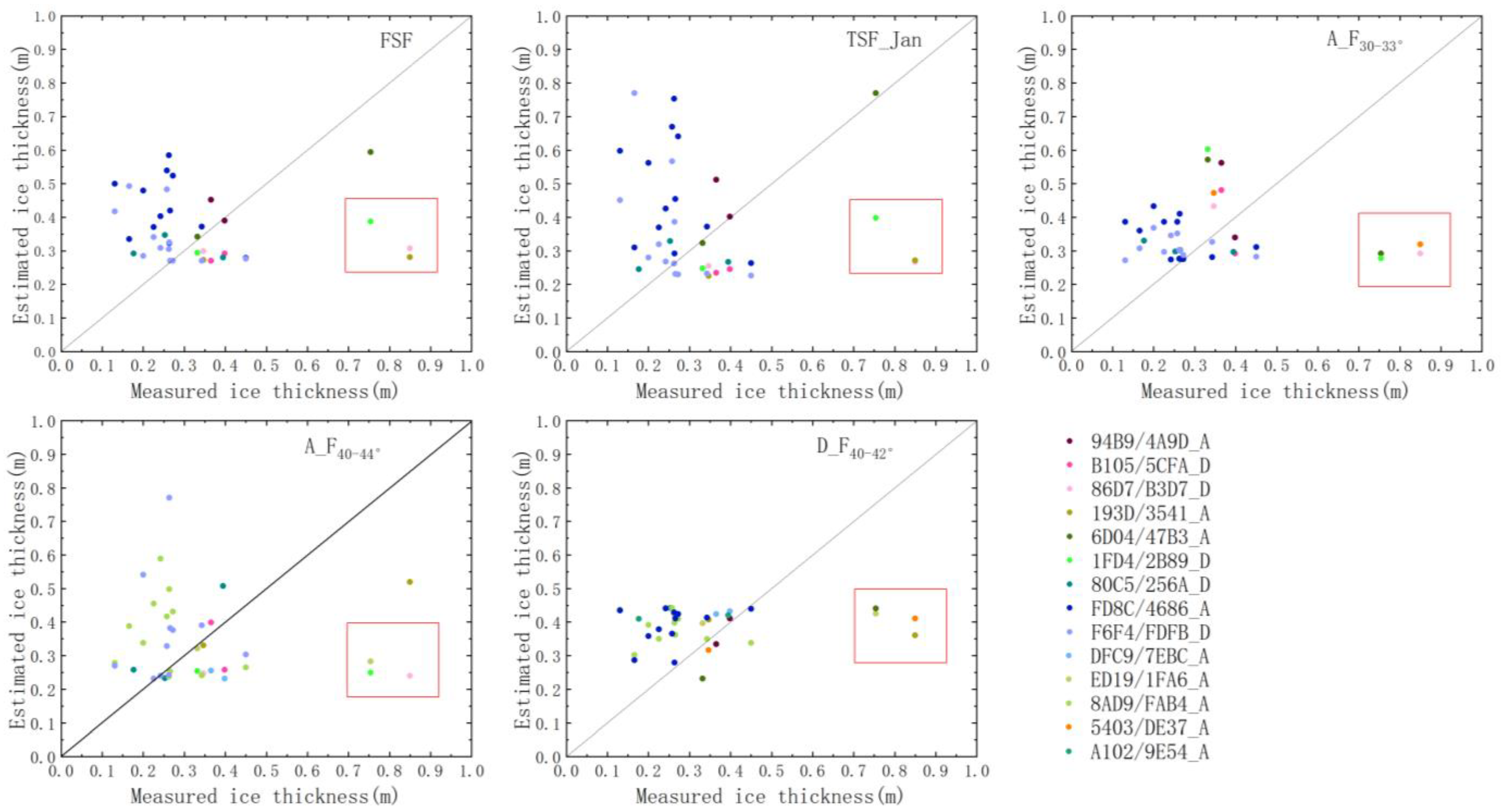
Figure 9 shows the measured and simulated values for the independent validation of each scheme, and the following results were obtained.
The FSF scheme is better suited for the January 2019 ascending orbit image (94B9/4A9D_A, brown dots). The equation is less accurate for radar images acquired during periods of thin river ice (FD8C/4686_A, F6F4/FDFB_D).
The TSF scheme, although it shows poor accuracy in the independent validation, and the TSF_Jan fitting equation, simulated by measured data during periods of thin river ice, are suitable for radar imagery during periods of thin river ice (80C5/256A_D).
Compared with the other equations, the A_F30–33° fitting equation is more suitable for river ice under different developmental states, and its simulated values are the closest to the 1:1 line. The A_F40–44° and D_F40–42° fitting equations can obtain good results for radar images in all periods except for the periods with thin river ice (8AD9/FAB4_A, F6F4/FDFB_D).
Figure 9 shows that the simulated values of the fitting equations deviate from the 1:1 line when the river ice thickness reaches a certain value. When the river ice thickness is greater than 0.75 m, the river ice thickness inverted by descending orbit radar images is not as good as that inverted by ascending orbit radar images. For river ice thicknesses greater than 0.80 m, the river ice inversion accuracies from both descending and ascending orbit radar images are poor (red boxes in Figure 9). In addition, the fitting equations do not work well for inverting thin river ice, such as in January 2021, when most measured thicknesses are less than 0.20 m (dark blue and light blue dots in Figure 9).
Therefore, the Babao River simulation schemes can be used for inverting river ice with a thickness of 0.20–0.80 m.

4.2. Binggou River

4.2.1. Scheme Fitting Effects

When the FSF scheme is used, the polarization parameter with the strongest correlation is α, with an R2 of 0.103 and L_RMSE of 0.285 m (Figure 10), stepwise regression RMSE is 0.281m (Figure 11). However, Figure 12a shows that when the measured thickness is greater than 0.90 m or less than 0.20 m, the simulation result is poor.
When using the TSF scheme, the polarization parameter with the strongest correlation for the January fitted equation (TSF_Jan) is the VH polarization mode, with an R2 of 0.130 and an L_RMSE of 0.179 m. The corresponding polarization parameter for the fitted equation for February through April (TSF_Feb–Apr) is α, with an R2 of 0.134 and an L_RMSE of 0.283 m.
When using the A/D_F scheme, the descending orbit images with a lower incidence angle (D_F30–33°) are more suitable for inverting the river ice thickness in the Binggou River, with an L_RMSE of 0.270 m, which is second only to that (0.179 m) of the TSF_Jan equation. For the descending orbit images with a higher incidence angle (D_F38–43°), the L_RMSE is 0.299 m, and for the ascending orbit images (A_F40–45°), the L_RMSE is 0.296 m. In the Binggou River, the descending orbit radar images with a lower incidence angle (D_F30–33°) are more suitable for inverting the river ice thickness. When stepwise regression is employed to perform the simulation (Figure 11), the RMSE of the multiparameter fitted equation (D_F30–33°) improves to 0.258 m. However, the other stepwise regression equations have no significant improvement in the simulation accuracy because they have only one fitted parameter.
In Figure 12, the values of the fitting equations of TSF_Jan and A_F40–45° are close to the 1:1 line only around 0.4 m, FSF and D_F30–33° can be well close to the 1:1 line within the range of 0.2–0.9 m. Of course, the values obtained from the stepwise regression (Figure 12e black dots) are significantly closer to the 1:1 line than the univariate regression (Figure 12e red dots).
Overall, the FSF, TSF_Jan, and D_F30–33° fitting equations are better and more suitable for inverting the river ice thickness in the Binggou River, and the descending radar images are better than the ascending radar images. Furthermore, multiple stepwise regression is better than univariate stepwise regression.
In addition, the high elevation of the Binggou River region (mean elevation of 3800 m) and the fact that most of the area is obscured by mountains cause the Sentinel-1 data with a 10 m spatial resolution to exhibit a less satisfactory performance. Hence, the results obtained for the Binggou River are relatively poor compared to those acquired for the Babao River, as the topography of the Binggou River is more complex, the channel is narrower, the ice is thicker, and the relationship with radar polarization parameters is more complex. However, with the support of publicly available radar data, it was found that some correlations could be found with the polarization parameters under the influence of topography, and some of the fitting equation results were acceptable.

4.2.2. Independent Validation of the Inversion Equations for the Binggou River

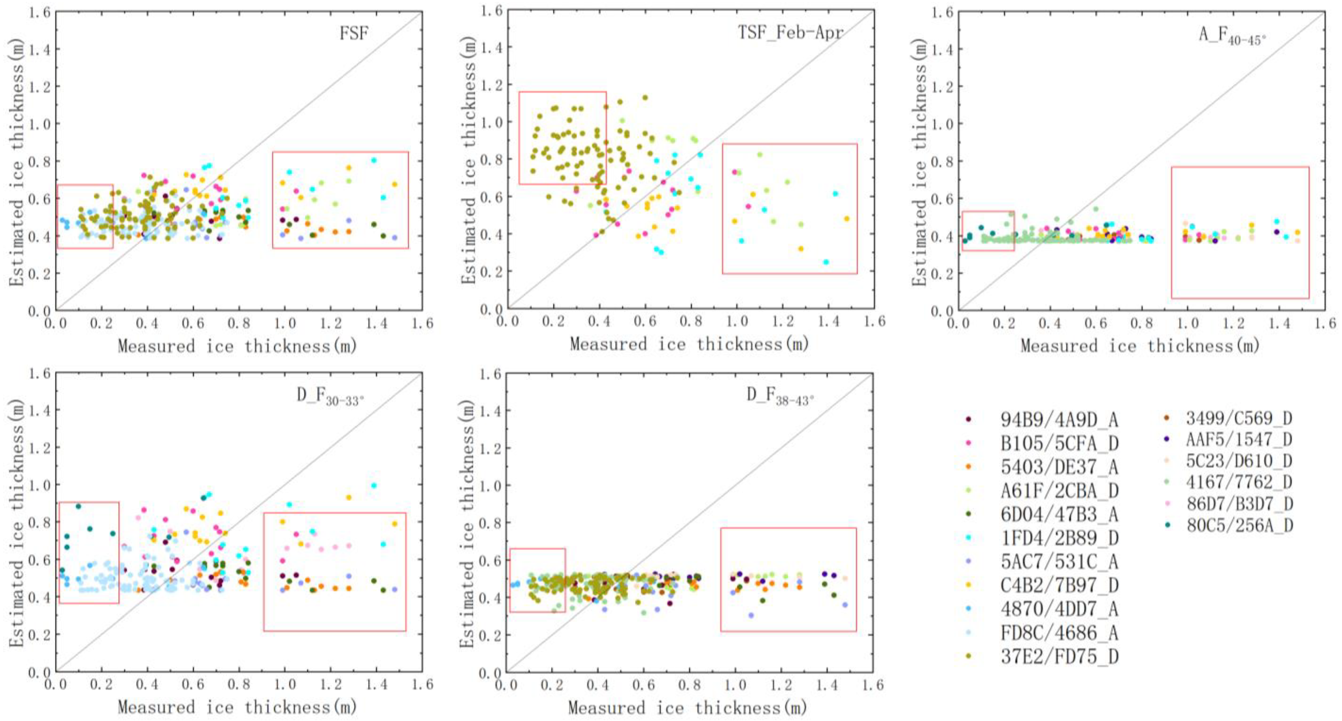
Similar to the Babao River analysis, the Binggou River inversion equations are independently verified. Figure 13 shows the measured, and simulated values for the independent validation of each fitting equation, and the results obtained are as follows.
The FSF, TSF, and D_F30–33° fitting equations are not suitable for radar images during periods of thin river ice (for example, 4870/4DD7_A, FD8C/4686_A, 37E2/FD75_D, 80C5/256A_D), although their accuracy improves in other periods.
The simulated values of the fitting equations deviate from the 1:1 line when the thickness of the river ice reaches a certain value. That is, the simulated values deviate from the 1:1 line (red boxes in Figure 13) when the river ice thickness is greater than 0.90 m or less than 0.20 m. For the ascending and descending orbit radar images, the accuracy of the independent verification of the descending orbit images is better than the accuracy of the ascending orbit images.
Figure 13 suggests that inverting the river ice thickness in the Binggou River is more feasible with descending orbit data (e.g., B105/5CFA_D), which is related to the direction of rivers. Overall, the Binggou River inversion schemes are more suitable for river ice with a thickness of 0.20–0.90 m. Nevertheless, the physical mechanisms responsible for the radar backscatter from significantly thinner or thicker river ice need to be further explored.

4.3. Intervalidation of the Babao River and Binggou River Schemes

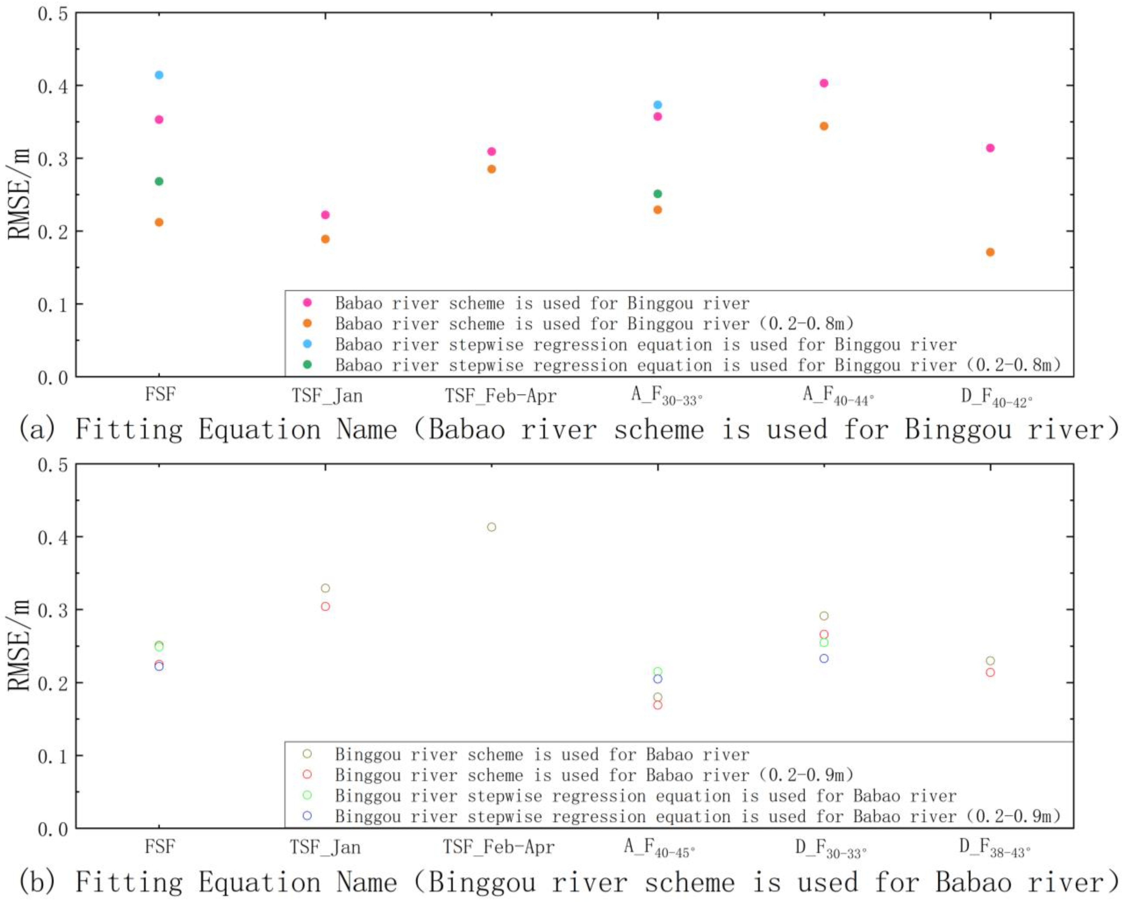
In this paper, the inversion schemes of different river levels are applied to each other. In other words, the inversion schemes of the Babao River are used for the Binggou River, and the inversion schemes of the Binggou River are used for the Babao River; the schemes exhibit a one-to-one correspondence. The mutual application of these schemes further considers the thickness inversion thresholds obtained in Section 4.1.2 and Section 4.2.2, which are 0.20–0.80 m and 0.20–0.90 m, respectively. Therefore, when the Babao River schemes are used in the Binggou River, the thickness is defined within the range of 0.20–0.80 m, and when the Binggou River schemes are used in the Babao River, the thickness is defined within the range of 0.20–0.90 m.
When applying the Babao River schemes to the Binggou River (solid dots in Figure 14a), the results are slightly better for the TSF_Jan and D_F40–42° fitting equations. The accuracy of the D_F40–42° simulation is improved to 0.171 m when the defined inversion range is 0.20–0.80 m, mainly because the descending orbit radar images are more suitable for inverting the river ice thickness in the Binggou River, as analyzed earlier, while the Babao River schemes have only one descending orbit fitting equation (D_F40–42°). Therefore, the Babao River D_F40–42° fitting equation achieves better accuracy in the Binggou River.
When applying the Binggou River schemes to the Babao River (hollow dots in Figure 14b), the accuracy of A_F40–45° is obviously better, with an RMSE of 0.180 m. When defining the thickness inversion range as 0.20–0.90 m (red hollow dots in Figure 14b), the accuracy of the A_F40–45° simulation is improved to 0.169 m. As analyzed above, ascending orbit radar images are more suitable for inverting the ice thickness in the Babao River, and the Binggou River schemes only have one ascending orbit fitting equation (A_F40–45°); therefore, compared with the other Binggou River schemes, A_F40–45° is more suitable for inverting the ice thickness in the Babao River.
Overall, the D_F40–42° fitting equation for the Babao River is more suitable for the Binggou River, and the A_F40–45° fitting equation for the Binggou River is more suitable for the Babao River.

4.4. Influence of River Ice Thickness on the Inversion Accuracy

The previous sections analyze the control range of the river ice thickness when the inversion equation is used in other radar images (0.20–0.80 m for the Babao River and 0.20–0.90 m for the Binggou River). This section focuses on the effect of variation in the river ice thickness on the inversion accuracy.
First, for the Babao River, Figure 15A shows the change in the simulation RMSE when the thickness of river ice changes, demonstrating that the simulation accuracy of TSF_Fep–Apr substantially improves when excluding data beyond 0.20–1 m, and the river ice is thickest in that period. In contrast, the other fitting equations, such as TSF_Jan, basically have no measured thicknesses exceeding 1 m, and thus, there is no significant change in the RMSE when excluding data beyond 0.20–1 m for these fitting equations. Therefore, the inversion equations for the Babao River are suitable for rivers with wide channels and thin river ice.
Second, for the Binggou River, Figure 15B similarly shows the RMSE variation when the river ice thickness changes. Except for the TSF_Fep–Apr fitting equation, all the fitting equations display a substantial increase in RMSE when controlling the river ice thickness in the range of 0.20–0.90 m. The RMSE of TSF_Fep–Apr does not change significantly, indicating that the higher simulated thicknesses (February to April) can be used to invert the Binggou River ice thickness during periods of thick river ice. In contrast, the other inversion equations for the Binggou River are suitable for inverting river ice thicknesses within 0.20–0.90 m.
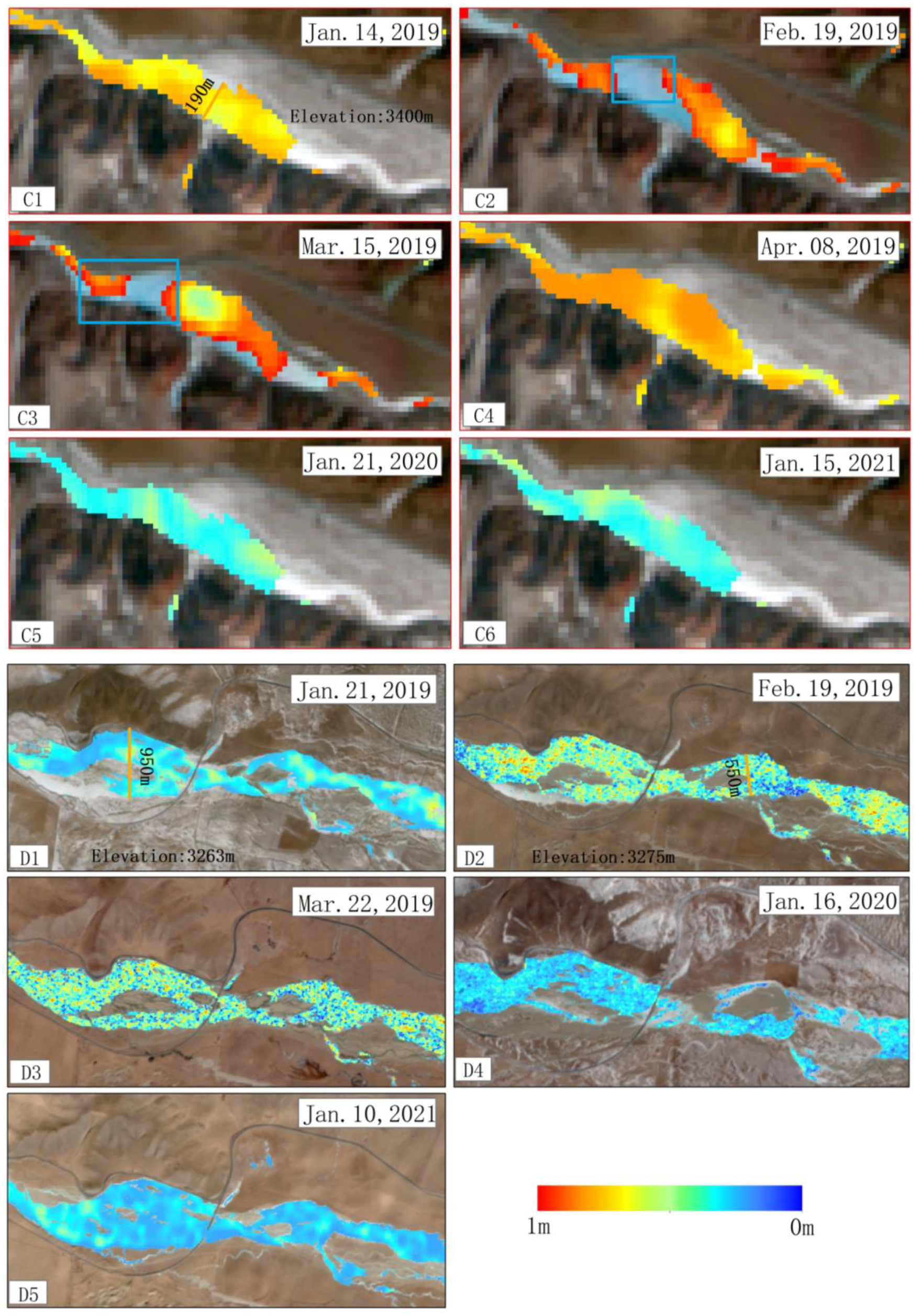
The inversion equations, combining the above analyses of fitting equations and thicknesses, were applied to radar images to obtain the spatial distributions of river ice thickness (Figure 15). The ice thickness in the Babao River (Figure 15(D1–D5)) and the Binggou River (Figure 15(C1–C6)) is thin in January and thickest in February and March, after which the thickness starts to decrease in April until it thaws completely. As shown in Figure 15, the inverted distributions of river ice thickness in the Babao River and Binggou River are relatively uniform, and some of the fitting equations match the measured values well (Figure 8 and Figure 12). However, in some areas of the Binggou River, the thickness of river ice is greater than 0.90 m, which diminishes the reliability of the simulated thicknesses (blue box in Figure 15(C3)). In addition, the uncertainty in the river ice backscattering on both sides of the river and on smoother river ice may lead to less reliable simulated values in these areas.

5. Discussion

5.1. Similarities and Differences with Existing Polarized River Ice Inversion Methods

Studies on river ice thickness have focused on large rivers in Canada [7,10,11,16]. Current methods for obtaining river ice thickness include the traditional borehole method and Stefan’s ice thickness formula based on hydrological data [13], in addition to inversion methods based on various sensors, such as airborne microwave scatterometer [27], ground-penetrating radar [9] and C-band synthetic aperture radar (e.g., RADARSAT). Previously, a nonlinear regression fitting equation was developed using the H of RADARSAT-2 as the independent variable [10] and the river ice thickness of the Koksoak River (Canada) with the following inversion equation:
h i = 0.55 H 2 + 1.57 H 0.09
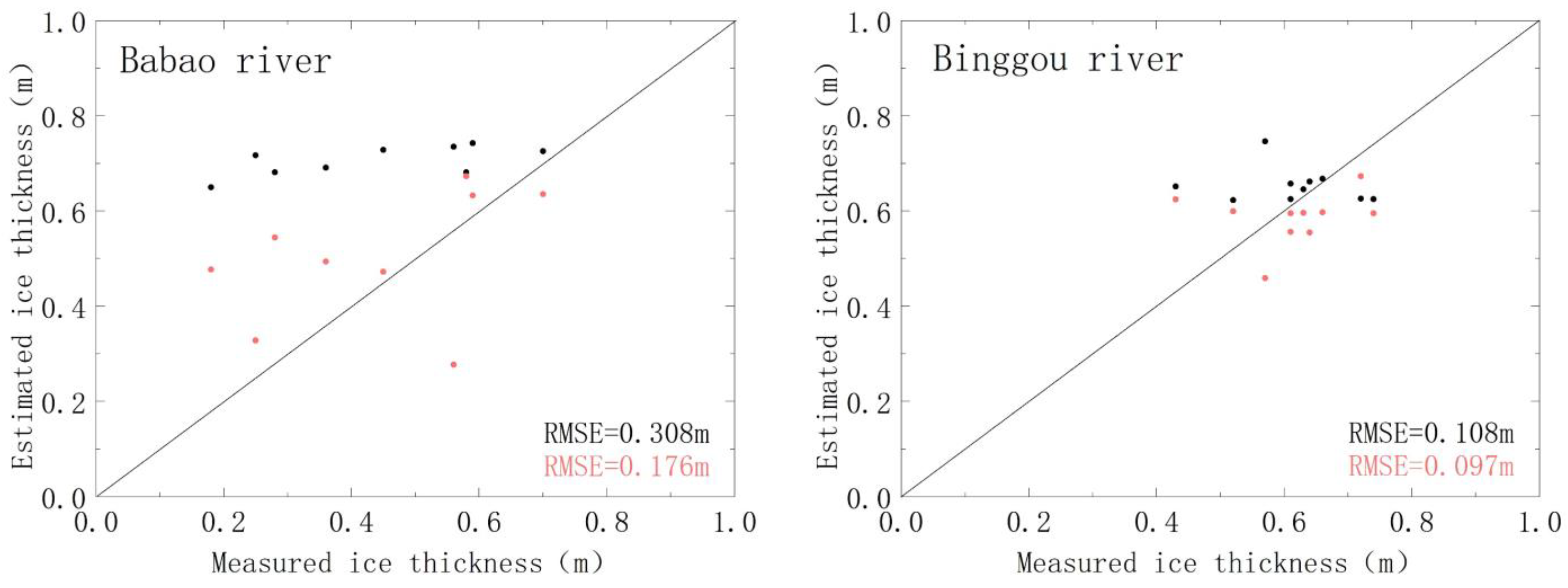
where H denotes entropy and hi denotes the simulated value. This equation is applicable to C-band radar images with an image incidence angle between 27° and 35°, an H range of 0.20–0.85, and an inversion thickness threshold of 0.80 m. In this paper, after filtering by the above conditions, 9 and 10 measured data points of the Babao River and Binggou River, respectively, meet these requirements. The values of these measurements are substituted into Equation (14), and the results are shown in Figure 16 (black dots). To compare Equation (14) with the inversion equations proposed in this paper, the equations that meet the conditions are selected in schemes 1–3 for inversion.
The RMSE of the Babao River is 0.308 m, and the accuracy of the Binggou River can reach 0.108 m. Although the amount of data used for the inversion is small, the difference between the inversion accuracies for the Babao River and Binggou River is large. The above fitting equation is simulated from large rivers in northern Canada, which are less affected by topography and elevation changes, and the inversion accuracy for large Canadian rivers can reach 0.092 m, while the ice in the Babao River is thinner than that in the Binggou River (minimum value of 0.18 m versus 0.43 m, respectively). Hence, the fitting equation is more suitable for the inversion of ice thickness in Binggou River.

5.2. Findings of This Study

In this study, river ice thickness was retrieved from dual-polarization Sentinel-1 data, which were newer and more readily available than RADARSAT. To date, while river ice studies have focused on RADARSAT data [10,16], the potential of Sentinel-1 to study the thickness of river ice is unknown.
The innovative discovery of this study is that the dual-polarized Sentinel-1 data has the potential to invert river ice thickness on the Tibetan Plateau. Previous studies on river ice thickness have focused on large Canadian rivers with channel widths of 400–3000 m [10], whereas in this paper, the river widths are less than 400 m, except for parts of the main stream of the Babao River. This study addresses a typical watershed on the Tibetan Plateau with relatively complex topography, narrow rivers, and completely frozen rivers in winter. No formally reported microwave inversion method for river ice thickness has been used in such an area. Furthermore, this study is more exhaustive considering the spatiotemporal distribution of the collected samples, and rivers of different scales are analyzed and compared. In-depth analyses incorporating factors such as radar image ascending or descending orbit and the incident angle, and it is concluded that Babao River is suitable for ascending orbit and Binggou River is suitable for descending orbit inversion. The observation angles of the objects in the ascending and descending orbits are different, and the details of the objects are also captured differently. Previous studies have shown the difference between ascending and descending orbits [28]. In the Binggou River, the channel is downward from south to north, so the descending orbit from north to south may observe more details. This may be why the Binggou River descending orbit data is better than the ascending orbit data. Overall, future studies comparing profiles of radar data will be beneficial in understanding the differences between ascending and descending collection and thick/thin covers.
The influence of river ice thickness on the inversion is systematically analyzed. Previous studies on river ice thickness have not performed a corresponding analysis on how river ice thickness affects the inversion accuracy, but this study reveals that excessively thick or thin river ice influences the inversion accuracy. In addition, radar backscatter is influenced by both the physical properties of river ice and the sensor characteristics, resulting in different responses of river ice to radar backscatter under different formation states [7,10,15,29], and previous studies have shown that the H is more sensitive to river ice thickness [10], which is consistent with the study of the Babao River in this article. However, the results of this paper for the Binggou River suggest that the backscatter coefficient α is more sensitive to river ice thickness. The reason for this difference may be the difference in the physical structure of the river ice; according to our field survey, the ice in the Babao River is thin and evenly distributed, with a thin layer of snow covering the surface, whereas ice in some areas of the Binggou River is thicker, and the ice surface is not uniform in height, has less snow, and is brighter. These differences may be responsible for the poor inversion results of the Binggou River.

5.3. Shortcomings and Prospects

In this paper, an empirical equation to invert river ice thickness using C-band radar data is analyzed. This equation can be effectively employed in this study area; when the river ice is fully developed, the average thickness can reach 0.54 m and 0.85 m (Figure 2), and the RMSE is 0.109 m and 0.258 m (Figure 7 and Figure 11), respectively, in the Babao River and Binggou River. It suggests that the inversion errors could be comparable with the actual river ice thickness. These errors majorly come from multi factors such as the development status of the river ice, the ascending and descending orbit of the radar image, and the incident angle, which we have discussed in the result. It further indicates that the uncertainties should be kept in mind when trying to draw further conclusions regarding ice thickness variations along the rivers using a similar inversion method. As our study indicates, the following factors should be paid attention to: (1) the development status of river ice; (2) radar image ascending or descending orbit; (3) radar image incident angle; (4) the width of the river channel and the type of river ice; and (5) the dielectric constant of river ice.
Barzegar et al. [11] used a new machine learning approach, namely, a bootstrap extreme learning machine (BELM) with a bootstrap least squares support vector machine (BLSSVM), to simulate the ice thicknesses in the Mackenzie and Yellowknife Rivers in the Northwest Territories, Canada. While their model is generalizable, it requires water flow, snow depth, and input variables such as mean air temperature. It is challenging to apply this approach to the Tibetan Plateau, where field data are difficult to obtain. The only more suitable method for inverting the river ice thickness on the Tibetan Plateau is the C-band SAR inversion method proposed by Mermoz et al. [10], but this method is not applicable to all types of river ice, and its generalizability needs further validation.
Therefore, based on the outcomes of previous studies, future work can be carried out in the following areas: (1) Develop inversion equations suitable for all river ice types on the Tibetan Plateau. The inversion equation simulated in this paper is suitable for snow ice in the Babao River, but the accuracy is not very satisfactory for consolidated ice, such as in certain areas of the Binggou River. Therefore, the internal characteristics of river ice (dielectric properties, etc.) must be better understood to develop a targeted inversion scheme. (2) Combine multiband radar images. From high to low, the penetrability of radar bands decreases in the order of L, S, C, and X, and thus, the relationships between different wavelengths and thickness inversion schemes can be explored using different bands to improve the fitting equation. (3) Consider other influencing factors to build the fitting equation. In this paper, only the development state of river ice is considered, but the temperature, precipitation, wind speed, etc., can also affect the river ice thickness inversion accuracy.

6. Conclusions

In this study, river ice thickness was retrieved from dual-polarization Sentinel-1 data, and the developmental state of river ice and radar images are taken into account to study two high-order rivers. The main conclusions are summarized as follows:
(1) Sentinel-1 C-band data can better invert river ice thickness in complex topographic areas. (2) H can better explain the river ice thickness for the Babao River, and the α angle performs better for Binggou River. (3) The thickness of river ice has an impact on the simulation accuracy, and the inversion schemes are more effective for 0.20–0.90 m river ice thickness. (4) East–west river channels (the Babao River) are more suitable for inversion using ascending radar data, whereas north–south river channels (the Binggou River) are more suitable for inversion using descending radar data. (5) Excluding the influence of multicollinearity, multiple stepwise regression can better invert the river ice thickness than linear or nonlinear univariate regression.
Our study indicates that the uncertainties should be kept in mind when trying to draw further conclusions using inversed ice thickness in high-order rivers. The uncertainties include the radar image ascending and descending orbit, incident angle, river ice development status, and river ice type. In addition, the physical properties of river ice, air temperature, precipitation, etc., could be combined to promote the development of highly generalizable inversion equations for the river ice thickness in high-order rivers.

Author Contributions

Conceptualization, H.Z. and H.L. (Hongyi Li); methodology, H.Z. and H.L. (Haojie Li); software, H.Z.; validation. H.Z.; formal analysis, H.Z. and H.L. (Hongyi Li); investigation, H.Z.; resources, H.L. (Haojie Li); data curation, H.Z. and H.L. (Hongyi Li); writing—original draft preparation, H.Z.; writing—review & editing, H.L. (Hongyi Li) and H.L. (Haojie Li); supervision, H.L. (Hongyi Li); projection administration, H.L. (Hongyi Li); funding acquisition, H.L. (Hongyi Li). All authors have read and agreed to the published version of the manuscript.

Funding

This research was funded by the National Natural Science Foundation of China (Grant Numbers: 41971399), the Natural Science Foundation of Qinghai Province (Grant Numbers: 2020-ZJ-731) and the Science & Technology Basic Resources Investigation Program of China (Grant Number: 2017FY100503).

Data Availability Statement

Sentinel-1 GRD data can be obtained from the ESA and Copernicus Sentinel Satellites Project using Google Earth Engine (https://developers.google.com/earth-engine/datasets/catalog/COPERNICUS_S1_GRD/, accessed on 1 March 2021). Sentinel-1 SLC data can be obtained from the ASF Data Search (https://search.asf.alaska.edu/, accessed on 1 March 2021).

Acknowledgments

We are grateful to the data providers. The data of the Babao River basin were provided by the National Tibetan Plateau/Third Pole Environment Data Center. The Sentinel-1 image sets used in this study are available on the ASF Data Search (https://search.asf.alaska.edu/, accessed on 1 March 2021).

Conflicts of Interest

The authors declare no conflict of interest.

References

  1. Cooley, S.W.; Pavelsky, T.M. Spatial and temporal patterns in Arctic river ice breakup revealed by automated ice detection from MODIS imagery. Remote Sens. Environ. 2016, 175, 310–322. [Google Scholar] [CrossRef]
  2. Li, H.; Li, H.; Wang, J.; Hao, X. Identifying river ice on the Tibetan Plateau based on the relative difference in spectral bands. J. Hydrol. 2021, 601, 126613. [Google Scholar] [CrossRef]
  3. Beaton, A.; Whaley, R.; Corston, K.; Kenny, F. Identifying historic river ice breakup timing using MODIS and Google Earth Engine in support of operational flood monitoring in Northern Ontario. Remote Sens. Environ. 2019, 224, 352–364. [Google Scholar] [CrossRef]
  4. Beltaos, S. Threshold between mechanical and thermal breakup of river ice cover. Cold Reg. Sci. Technol. 2003, 37, 1–13. [Google Scholar] [CrossRef]
  5. Muhammad, P.; Duguay, C.; Kang, K.K. Monitoring ice break-up on the Mackenzie River using MODIS data. Cryosphere 2016, 10, 569–584. [Google Scholar] [CrossRef] [Green Version]
  6. Li, H.; Li, H.; Wang, J.; Hao, X. Monitoring high-altitude river ice distribution at the basin scale in the northeastern Tibetan Plateau from a Landsat time-series spanning 1999–2018. Remote Sens. Environ. 2020, 247, 111915. [Google Scholar] [CrossRef]
  7. Jasek, M.; Weber, F.; Hurley, J. Ice Thickness and Roughness Analysis on the Peace River using RADARSAT-1 SAR Imagery. In Proceedings of the 12th Workshop on the Hydraulics of Ice Covered Rivers, Edmonton, AB, Canada, 19–20 June 2003. [Google Scholar]
  8. Mermoz, S.; Allain, S.; Bernier, M.; Pottier, E. Investigation of Radarsat2 and TerraSAR-X data for river ice classification. In Proceedings of the Geoscience & Remote Sensing Symposium, Cape Town, South Africa, 12–17 July 2009. [Google Scholar]
  9. Kämäri, M.; Alho, P.; Colpaert, A.; Lotsari, E. Spatial variation of river-ice thickness in a meandering river. Cold Reg. Sci. Technol. 2017, 137, 17–29. [Google Scholar] [CrossRef]
  10. Mermoz, S.; Allain-Bailhache, S.; Bernier, M.; Pottier, E.; Van Der Sanden, J.J.; Chokmani, K. Retrieval of River Ice Thickness From C-Band PolSAR Data. IEEE Trans. Geosci. Remote Sens. 2014, 52, 3052–3062. [Google Scholar] [CrossRef] [Green Version]
  11. Barzegar, R.; Ghasri, M.; Qi, Z.; Quilty, J.; Adamowski, J. Using bootstrap ELM and LSSVM models to estimate river ice thickness in the Mackenzie River Basin in the Northwest Territories, Canada. J. Hydrol. 2019, 577, 123903. [Google Scholar] [CrossRef]
  12. Luo, S.; Song, C.; Zhan, P.; Liu, K.; Chen, T.; Li, W.; Ke, L. Refined estimation of lake water level and storage changes on the Tibetan Plateau from ICESat/ICESat-2. Catena 2021, 200, 105177. [Google Scholar] [CrossRef]
  13. Zhi-Jun, L.I.; Sun, W.G.; Shi-Guo, X.U.; Qing-Shan, L.I.; Bai, Y.; Wang, X. Calculating river ice thickness from Harbin to Tongjiang using short-term hydrological and meteorological data. Adv. Water Sci. 2009, 20, 428–433. [Google Scholar]
  14. Chu, T.; Lindenschmidt, K.-E. Integration of space-borne and air-borne data in monitoring river ice processes in the Slave River, Canada. Remote Sens. Environ. 2016, 181, 65–81. [Google Scholar] [CrossRef]
  15. Unterschultz, K.D.; van der Sanden, J.; Hicks, F.E. Potential of RADARSAT-1 for the monitoring of river ice: Results of a case study on the Athabasca River at Fort McMurray, Canada. Cold Reg. Sci. Technol. 2009, 55, 238–248. [Google Scholar] [CrossRef]
  16. Lindenschmidt, K.-E.; Syrenne, G.; Harrison, R. Measuring Ice Thicknesses along the Red River in Canada Using RADARSAT-2 Satellite Imagery. J. Water Resour. Prot. 2010, 2, 923–933. [Google Scholar] [CrossRef] [Green Version]
  17. Puestow, T.M.; Randell, C.J.; Rollings, K.W.; Khan, A.; Picco, R. Near real-time monitoring of river ice in support of flood forecasting in eastern Canada: Towards the integration of Earth observation technology in flood hazard mitigation. In Proceedings of the IEEE International Geoscience & Remote Sensing Symposium, Anchorage, AK, USA, 20–24 September 2004. [Google Scholar]
  18. Toyota, T.; Ono, S.; Cho, K.; Ohshima, K.I. Retrieval of sea-ice thickness distribution in the Sea of Okhotsk from ALOS/PALSAR backscatter data. Ann. Glaciol. 2011, 52, 177–184. [Google Scholar] [CrossRef] [Green Version]
  19. Sanden, J.; Drouin, H. Satellite SAR Observations of River Ice Cover: A RADARSAT-2 (C-band) and ALOS PALSAR (L-band) Comparison. In Proceedings of the 16th Workshop on River Ice, Winnipeg, MB, Canada, 18–22 September 2011. [Google Scholar]
  20. Li, H.; Li, H.; Wang, J.; Hao, X. Extending the Ability of Near-Infrared Images to Monitor Small River Discharge on the Northeastern Tibetan Plateau. Water Resour. Res. 2019, 55, 8404–8421. [Google Scholar] [CrossRef]
  21. Yang, X.; Pavelsky, T.M.; Allen, G.H. The past and future of global river ice. Nature 2020, 577, 69–73. [Google Scholar] [CrossRef]
  22. Lee, J.S.; Grunes, M.R.; Grandi, G. Polarimetric SAR speckle filtering and its implication for classification. IEEE Trans. Geosci. Remote Sens. 2002, 37, 2363–2373. [Google Scholar]
  23. Gouveia, N.D.A.; Alves, F.C.; Pereira, L.D.O. Pre-processing of Sentinel-1 C-band SAR images based on incidence angle correction for dark target detection. Remote Sens. Lett. 2019, 10, 939–948. [Google Scholar] [CrossRef]
  24. Ji, K.; Wu, Y. Scattering Mechanism Extraction by a Modified Cloude-Pottier Decomposition for Dual Polarization SAR. Remote Sens. 2015, 7, 7447–7470. [Google Scholar] [CrossRef] [Green Version]
  25. Harfenmeister, K.; Itzerott, S.; Weltzien, C.; Spengler, D. Agricultural Monitoring Using Polarimetric Decomposition Parameters of Sentinel-1 Data. Remote Sens. 2021, 13, 575. [Google Scholar] [CrossRef]
  26. Hong, R.; Guo, X.; Tu, J.; Rui, Z. The Water Extraction and Flood Season Changes Detection of Poyang Lake Based on Dual Polarized Sentinel-1A Image Data. Geomat. Sci. Technol. 2018, 6, 298–308. [Google Scholar] [CrossRef]
  27. Han, H.S.; Kim, B.J.; Lee, H.Y. A Study on the Measurement of River Ice Thickness by Using X-band Scatterometer. Geophys. Geophys. Explor. 2012, 15, 16–22. [Google Scholar] [CrossRef]
  28. Dumitru, C.O.; Datcu, M. Information Content of Very High Resolution SAR Images: Study of Feature Extraction and Imaging Parameters. IEEE Trans. Geosci. Remote Sens. 2013, 51, 4591–4610. [Google Scholar] [CrossRef]
  29. Gherboudj, I.; Bernier, M.; Leconte, R. A Backscatter Modeling for River Ice: Analysis and Numerical Results. IEEE Trans. Geosci. Remote Sens. 2010, 48, 1788–1798. [Google Scholar] [CrossRef]
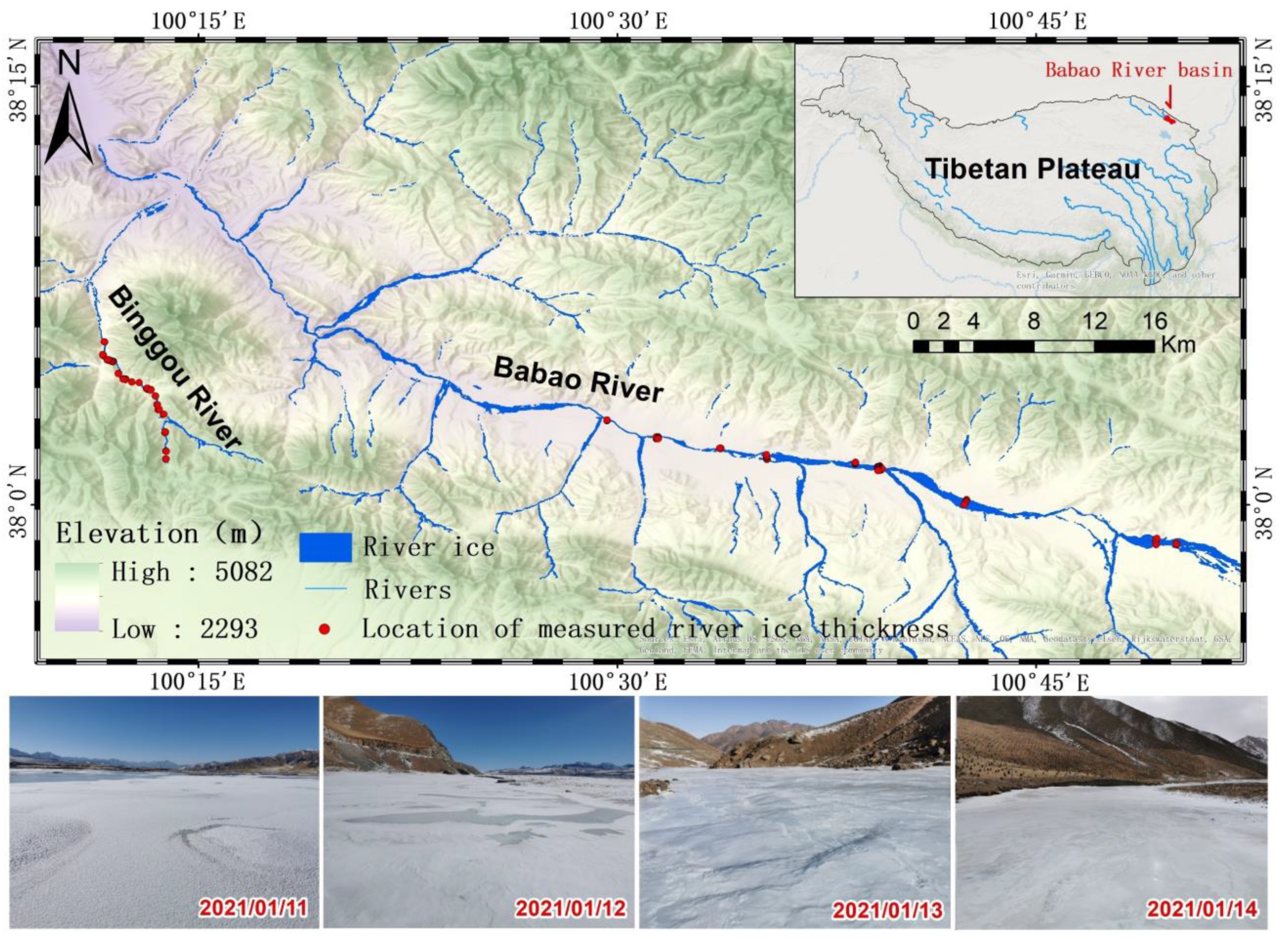
Figure 1. Overview of the study area of the Babao River basin and a map of its river ice distribution. The four photos demonstrate the status of river ice: The first two show the main stream of the Babao River, while the last two show that of the Binggou River. The locations of the river ice sampling points are indicated in the figure, and the red area in the upper-right inset delineates the location of the Babao River basin on the Tibetan Plateau.
Remotesensing 14 02591 g001
Figure 2. Daily average intervals of the measured river ice thicknesses during 2019–2021. The black dashed line indicates the dividing line between the Babao River and the Binggou River; for the horizontal coordinates, orange indicates 2019, fluorescent blue indicates 2020, and green indicates 2021.
Remotesensing 14 02591 g002
Figure 3. Dates on which Sentinel-1 measured the river ice thickness during 2019–2021. The Babao River data are represented by diamonds, and the Binggou River data are represented by circles; blue indicates ascending, and orange indicates descending (for example, B105/5CFA indicates the acquired GRD/SLC data).
Remotesensing 14 02591 g003
Figure 4. Main scheme framework. FSF means all samples are fitted; TSF_Jan means that data measured in January are fitted, where Jan denotes January; TSF_Feb–Apr means that data measured in February, March, and April are fitted (the river ice thickness is 0 in April in the Babao River); and in scheme 3, A_F30–33°, A_F40–44°, and D_F40–42° are the Babao River fitting equations, and A_F40–45°, D_F30–33°, and D_F38–43° are the Binggou River fitting equations (for example, in A_F30–33°, A means ascending orbit, D means descending orbit, F denotes fitting, and 30–33° is the radar image incidence angle range).
Remotesensing 14 02591 g004
Figure 5. Framework for implementing the proposed process. The polarization parameters (entropy, anisotropy, and scattering angle) are obtained by preprocessing, such as orbit correction, polarization filtering, terrain correction, and polarization decomposition, and the three inversion schemes, FSF, TSF, and A/D_F, are designed for univariate regression and stepwise regression. The orange color indicates the Babao River, and the purple color indicates the Binggou River.
Remotesensing 14 02591 g005
Figure 6. Linear and nonlinear fitting equations for the Babao River. Orange, yellow, and blue indicate the methods with better accuracy for each scheme. Two-tailed, 95% confidence interval. * represents a significant correlation at the 0.05 level. ** represents a significant correlation at the 0.01 level. Entropy is denoted H, and anisotropy is denoted A. Rectangular boxes indicate simulations using H, rounded boxes indicate simulations using VH, and pointed boxes indicate simulations using VV. The polarization methods of the FSF and TSF schemes use images that are ascending orbits close to the acquisition date, while that of the A/D_F scheme divides images according to the ascending orbit, descending orbit, and incidence angle. The thickness of river ice in April in the Babao River is 0.
Remotesensing 14 02591 g006
Figure 7. Stepwise regression fitting equations for the Babao River. H_A denotes the entropy of an ascending orbit image, VH_A denotes the VH polarization of an ascending orbit image, and VH_D is the VH polarization of a descending orbit image. The orange and blue colors indicate the methods with the best accuracy.
Remotesensing 14 02591 g007
Figure 8. Comparison between the measured and simulated ice thicknesses in the Babao River (1:1 line), with the red dots indicating the univariate regression results and the black dots indicating the stepwise regression results. The red boxes indicate the univariate regression-simulated indicators, while the black boxes indicate the stepwise regression-simulated indicators. The panels are lettered a through f from left to right, top to bottom. (a) FSF; (b) TSF_Jan; (c) TSF_Feb–Apr; (d) A_F30–33°; (e) A_F40–44°; (f) D_F40–42°.
Remotesensing 14 02591 g008
Figure 9. Analysis of the applicability of the Babao River schemes. In the figure legend, for example, in 94B9/4A9D_A, 4A9D indicates the image name, where A indicates an ascending orbit (refer to Figure 3).
Remotesensing 14 02591 g009
Figure 10. Linear or nonlinear fitted equations for the Binggou River. Two-tailed, 95% confidence interval. * represents significant correlation at the 0.05 level. ** represents significant correlation at the 0.01 level. Entropy is denoted as H, and anisotropy is denoted as A. Rectangular boxes indicate simulations using A, rounded boxes indicate simulations using VH polarization, and pointed boxes indicate scattering angle simulations. The orange, yellow, and blue colors indicate the methods with better accuracy for each scheme. FSF and TSF schemes use images with better correlation for the polarization method, and A/D_F divides the ascending orbit, descending orbit and incidence angle images.
Remotesensing 14 02591 g010
Figure 11. Stepwise regression fitting equations for the Binggou River. VH_D is the VH polarization of the descending orbit image, VV_D is the VV polarization of the descending orbit image, and Alpha_D is the descending orbit scattering angle. The orange and blue colors indicate the method with better accuracy for each scheme.
Remotesensing 14 02591 g011
Figure 12. Comparison between the measured and simulated ice thicknesses in the Binggou River, with red dots indicating the univariate regression results and the black dots indicating the stepwise regression results. The red boxes indicate the univariate regression-simulated metrics, while the black boxes indicate the stepwise regression-simulated metrics. The panels are lettered a through f from left to right, top to bottom. (a) FSF; (b) TSF_Jan; (c) TSF_Feb–Apr; (d) A_F40–45°; (e) D_F30–33°; (f) D_F38–43°.
Remotesensing 14 02591 g012
Figure 13. Analysis of the applicability of the Binggou River schemes. For example, 94B9/4A9D_A in the figure legend, 4A9D indicates the image name, and A indicates an ascending orbit (refer to Figure 3).
Remotesensing 14 02591 g013
Figure 14. Comparison of the inversion accuracies obtained by applying different river-level inversion equations to the other region. The above figure shows the simulation accuracies of the equations applied to both regions; the horizontal coordinate shows the name of the fitting equation for each scheme, and the vertical coordinate is the simulation RMSE. (a) Babao River scheme is used for Binggou River; (b) Binggou River scheme is used for Babao River.
Remotesensing 14 02591 g014
Figure 15. Effect of river ice thickness on the RMSE with the spatial distribution of river ice thickness. Panels (A,B) are plots reflecting the effect of river ice thickness on the RMSE, while (C1C6,D1D5) are maps of the spatial distribution of river ice thickness in individual areas. The orange line indicates the width of the river; the blue boxes indicate the areas with large inversion errors.
Remotesensing 14 02591 g015aRemotesensing 14 02591 g015b
Figure 16. Comparison between predicted and measured thicknesses (black dots represent the inversion results of the Canadian formula, while orange dots are the inversion formula results from this paper).
Remotesensing 14 02591 g016
Publisher’s Note: MDPI stays neutral with regard to jurisdictional claims in published maps and institutional affiliations.