Article

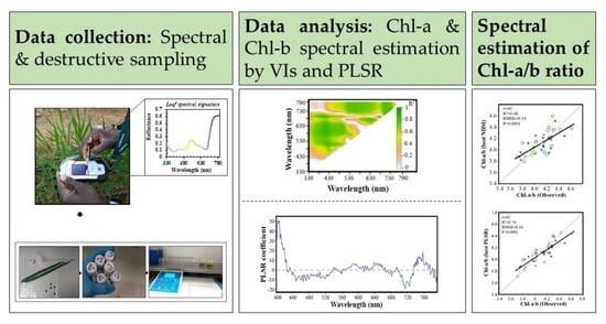
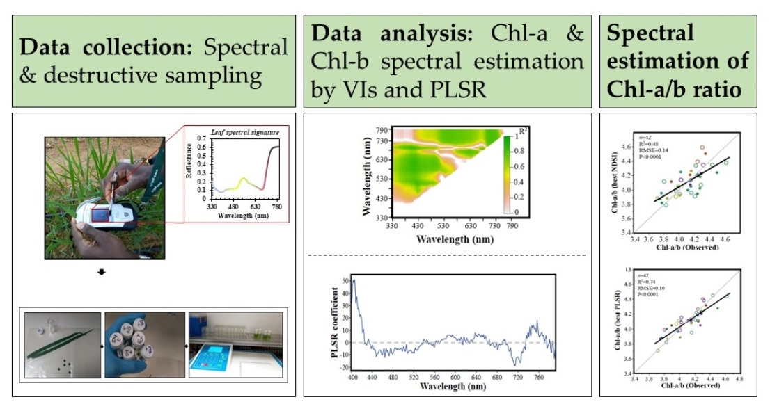
Spectral Estimation of In Vivo Wheat Chlorophyll a/b Ratio under Contrasting Water Availabilities

The Robert H. Smith Institute of Plant Sciences and Genetics in Agriculture, The Hebrew University of Jerusalem, Rehovot 7610001, Israel
*
Author to whom correspondence should be addressed.
Remote Sens. 2022, 14(11), 2585; https://doi.org/10.3390/rs14112585
Submission received: 23 April 2022 / Revised: 24 May 2022 / Accepted: 25 May 2022 / Published: 27 May 2022
(This article belongs to the Section Remote Sensing in Agriculture and Vegetation)

Abstract

:
To meet the ever-growing global population necessities, integrating climate-change-relevant plant traits into breeding programs is required. Developing new tools for fast and accurate estimation of chlorophyll parameters, chlorophyll a (Chl-a) content, chlorophyll b (Chl-b) content, and their ratio (Chl-a/b), can promote breeding programs of wheat with enhanced climate adaptability. Spectral reflectance of leaves is affected by changes in pigment concentration and can be used to estimate chlorophyll parameters. The current study identified and validated the top known spectral indices and developed new vegetation indices (VIs) for Chl-a and Chl-b content estimation and used them to non-destructively estimate Chl-a/b values and compare them to hyperspectral estimations. Three wild emmer introgression lines, with contrasting drought stress responsiveness dynamics, were selected. Well-watered and water-limited irrigation regimes were applied. The wheat leaves were spectrally measured with a handheld spectrometer to acquire their reflectance in the 330 to 790 nm range. Regression models based on calculated VIs as well as all hyperspectral curves were calibrated and validated against chlorophyll extracted values. The developed normalized difference spectral indices (NDSIs) resulted in high accuracy of Chl-a (NDSI415,614) and Chl-b (NDSI406,525) estimation, allowing for indirect non-destructive estimation of Chl-a/b with root mean square error (RMSE) values that could fit 6 to 10 times in the range of the measured values. They also performed similarly to the hyperspectral models. Altogether, we present here a new tool for a non-destructive estimation of Chl-a/b, which can serve as a basis for future breeding efforts of climate-resilient wheat as well as other crops.

Graphical Abstract

1. Introduction

Current and projected climate change, as expressed in the increasing intensity of erratic climate events across extensive regions of the planet, threatens to increase food insecurity worldwide [1]. To meet the ever-growing global population demands for food, feed, fibers, and bioenergy plant-based products, a significant increase in crop-plant production is required [2]. Thus, there is an urgent need to develop climate-resilient crop-plants with enhancing yield and nutritional quality for the changing agro-systems. A fundamental aspect of such an effort is the identification of key functional traits that can be integrated into research and breeding programs.
Chlorophyll is an important light-absorbing photosynthetic pigment largely determining the plant’s photosynthetic capacity and as consequence its growth and development [3]. It includes the chlorophyll a (Chl-a), which is the primary electron donor within the reaction center, and chlorophyll-b (Chl-b), a light-harvesting accessory pigment found in the antenna complexes of the light-harvesting complexes of photosystem II [4,5]. The ratio between chlorophyll a and b (Chl-a/b) is affected by the plant’s natural senescence processes and various environmental cues [6]. Under water stress, the Chl-b is degrading into Chl-a, leading to a higher Chl-a/b [7]. Thus, developing new tools for fast and accurate estimation of chlorophyll parameters can promote breeding efforts of new cultivars better adapted to the changing climate.
Quantification of leaf chlorophyll content was established by integrating empirical models of spectrophotometry measurement of light transmission wavelengths based on the Beer–Lambert law [8,9]. While resulting in accurate chlorophyll content, they are destructive, labor-intensive, time-consuming, and do not allow one to study the longitudinal and spatio-temporal dynamics thorough the plant’s life cycle [10,11,12]. Alternatively, an in vivo non-destructive optical hand-held absorbance-based total chlorophyll (TChl) meter (such as SPAD-502; Minolta corporation Ltd., Osaka, Japan) can be used. It can obtain a quick prediction of TChl content, but in many cases, the SPAD values are not calibrated to actual TChl content [13,14], and cannot estimate Chl-a, Chl-b and their ratio. Hyperspectral data are an alternative non-destructive approach, based on extracting reflectance values for hundreds of narrow spectral bands [15,16,17]. These data can be used for building models to determine TChl, Chl-a and Chl-b content as well as Chl-a/b. Spectral reflectance of leaves in the visible range and pigment concentration are negatively correlated [18,19,20,21]. A vegetation index (VI) is a mathematical manipulation based on reflectance values from two or more spectral bands [22] used to estimate plant traits and monitor their health and condition [23]. Spectral data and VIs are analyzed to estimate chlorophyll content in vegetation [5,24,25,26,27,28,29].
Wheat (Triticum sp.) is one of the world’s most consumed crops, with production estimated at ~770 million tons per annum http://www.fao.org/faostat (accessed on 20 February 2022). To meet the rising demand of the projected 9.7 billion people by 2050, an increase of at least 60% in wheat production is required [30]. Wheat domestication and subsequent evolution under domestication involved a suite of complex genetic, morphological, anatomical, and physiological modifications [31,32]. Wild emmer wheat (T. turgidum ssp. dicoccoides (Körn.) Thell.), the direct allotetraploid (2n = 4x = 28; genome BBAA) progenitor of domesticated wheats, thrives across wide eco-geographic amplitude across the Fertile Crescent and offers ample allelic repertoire for agronomically important traits, including drought tolerance [33,34,35]. Recently, we evaluated a large set of wild emmer wheat introgression lines (ILs) under contrasting water availabilities and identified promising drought tolerance strategies [33,34].
In the current study, we applied a field-based evaluation of selected ILs with divergent water-stress responsiveness and tested their Chl-a/b ratio alteration in response to water stress. Our working hypothesis was that Chl-a/b can be assessed non-destructively in in vivo wheat leaves based on Chl-a and Chl-b contents. The specific objectives of the current study were to: (i) identify and validate the best VIs for Chl-a and Chl-b, (ii) use the best VIs to assess Chl-a/b under contrasting water availabilities, and (iii) compare VIs- and hyperspectral- based Chl-a/b estimation models. Altogether, we showed here for the first time, to the best of our knowledge, a new tool, based on a spectral assessment of Chl-a and Chl-b for non-destructive estimation of Chl-a/b that can serve as a basis for future breeding efforts of climate-resilient wheat, as well as other crops.

2. Materials and Methods

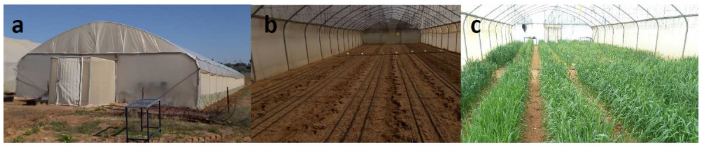
2.1. Plant Material and Experimental Design

Previously, we characterized a set of adaptive wild emmer wheat ILs (BC3F5) for their drought responsiveness strategies [33]. For the current study, we selected three lines (IL46, IL82, IL105) with contrasting drought stress responsiveness dynamics [33]. Each line consists of a few introgressions from the wild emmer line Zavitan, with IL46 consisting of six introgressions that cover 5.2% of the genome, IL82 consisting of fifteen introgressions that cover 13.37% of the genome, and IL105 consisting of six introgressions that cover 6.07% of the genome (Supplementary Table S1). IL46 was characterized as highly productive and stable and exhibited high growth and gas exchange under water stress. IL82 was characterized as highly productive and exhibited high growth under water stress with phenotypic plasticity (i.e., its physiological and morphological parameters were changing due to the water stress). IL105 was characterized to have lower biomass productivity under water stress and define as high phenotypic plasticity.
The plants were grown during the winter of 2019–2020 at the experimental farm of The Hebrew University of Jerusalem in Rehovot, Israel (34°47′N, 31°54′E: 54 m above sea level) in a plastic-covered net house (Figure 1). The soil is brown-red degrading sandy soil (Rhodoxeralf) composed of 76% sand, 8% silt, and 16% clay. A split-plot factorial (genotype x irrigation regime) design was employed with two irrigation regimes split into 12 sub-plots, with four replicates (total 24 plots). Each plot of 150 cm long consisted of four planted rows. Plants were spaced 10 cm, within and between rows, resulting in 60 plants per plot. Two irrigation regimes were applied via a drip irrigation system: well-watered control (WW) and water-limited (WL). The WW treatment was irrigated weekly with a total amount of ~750 mm, whereas the WL treatment was irrigated every other week with a total amount of ~250 mm (Supplementary Figure S1). Water was applied during the winter months (January–March) to mimic the natural pattern of rainfall in the eastern Mediterranean region. The experiment was treated with fungicides and pesticides to control fungal pathogens or insect pests and was weeded manually once a week.

2.2. Data Collection

Spectral data were acquired by PolyPen RP410 UVIS (PSI Ltd., Drasov, Czech Republic) in contact with the adaxial leaf side. The PolyPen is a leaf contact active spectrometer covering the range of 330 to 790 nm in 1 nm intervals (8 nm band width at full width half max). Before spectral data collection and in between measurements, a white reference measurement was acquired using a spectralon panel (PSI Ltd., Drasov, Czech Republic). Each selected leaf was in vivo spectrally measured five times to result in an average spectrum. The youngest fully developed leaf was selected for spectral data collection and sampling, while the flag-leaf was measured starting from the third until the ninth measuring date. In each plot, three leaves from different plants were marked and spectrally measured to represent the plot. The spectral data acquisition was followed by leaf sample collection. The leaves were cut from the plant into an air-tight polyethylene sealed bag and then placed into an ice-filled container for up to 2 h before further laboratory measurements.
Five leaf discs (0.8 cm diameter) were taken from each leaf and placed in a glass container with 10 mL of organic solvent (N.N Dimethylformamide) and transported into a dark 4 °C incubator for 48 h. Then, the samples were pipetted into 3 mL quartz cuvettes in the UV/VIS Spectrophotometer (ST-VS-723; Lab-Fac instrument Ltd., Kowloon, Hong Kong) to acquire transmittance in two wavelengths: 647 and 664 nm. The transmittance values were used to calculate the Chl-a, Chl-b, and TChl content (mg cm−2), as described previously [8]. Three plants per plot were sampled, the spectral and chlorophyll contents were averaged per plot.

2.3. Data Preprocessing and Analyses

Analysis of variance (ANOVA) was used to assess the possible effects of genotype, irrigation regimes, data collection dates, and the different levels of interactions on the chlorophyll responses.
Thirty-three well-known VIs were pre-programmed to be calculated by the PolyPen sensor (Supplementary Table S2). The quality of the correlation between each of the VIs and Chl-a, Chl-b, and TChl content was evaluated by the correlation coefficient (R). VIs resulting in R absolute values equal to or higher than 0.5 were selected for linear regression to produce a coefficient of determination (R2) and root mean square error of prediction (RMSEP). Data sets were randomly selected with an even distribution on genotype by irrigation regime by date for all parameters based on the number (n) of samples involved; Chl-a (n = 168), Chl-b (n = 167) and TChl (n = 166), at a 70% and 30%, calibration and validation, respectively. The calibration data sets were used to perform a linear regression analysis between Chl-a, Chl-b, and TChl content (dependent) and each of the selected VI (independent) variables and to determine the slope and intercept to be tested by the validation data sets. The predicted Chl-a, Chl-b, and TChl content values were compared to the observed values to obtain the calibration and validation R2 (Cal and Val R2, respectively) as well as RMSEP of calibration and validation (RMSEPC and RMSEPV, respectively) as calculated by Herrmann et al. [36]. The % RMSEPC and % RMSEPV were calculated based on the RMSEPC and RMSEPV values out of the range of Cal and Val samples, respectively. The statistical analyses were applied in JMP 15 pro version statistical package (SAS Institute, Cary, NC, USA).
To find the best two-band combination for Chl-a, Chl-b, and TChl content spectral estimation, the normalized difference spectral index (NDSI; [37]) was calculated, analyzed and ranked based on R2 values of a linear regression between Chl-a, Chl-b, and TChl content (Supplementary Table S2). The highly ranked NDSI for each of the three chlorophyll parameters (i.e., Chl-a, Chl-b, and TChl content) was used for the calibration and validation process as done with all selected VIs. The models’ quality was assessed by R2, RMSE and % RMSE. NDSI analysis was performed in R (version 3.4.1.) environment and statistical analyses were applied in JMP 14 pro version statistical package (SAS Institute, Cary, NC, USA).
In spectral data sets, as in the current study, there is high collinearity among variables (i.e., adjacent wavelengths), and partial least squares regression (PLSR) is a commonly applied method [38,39,40] that used the information at all wavelengths to provide a quantitative determination of plant traits. To calculate the estimated trait by the regression equation, each wavelength receives a coefficient; the absolute value of these coefficients indicates the importance of each wavelength to the model. The Cal and Val sample distributions were the same for the VIs analysis, and the models’ quality was assessed by R2, RMSE and % RMSE. The statistical analysis was performed in python 3.8 with pandas [41], version 1.3, SciPy [42], version 1.6, and scikit-learn [43], version 0.24, PLSR with NIPALS algorithm.

3. Results and Discussion

To test the effect of water availability on the accuracy of various non-destructive spectral models to estimate the Chl-a/b ratio, we used three selected wild emmer wheat introgression lines (ILs) that represent contrasting stress responsiveness strategies (L46, IL82 and IL105; see [33]). Characterization of these ILs under two contrasting water availabilities showed a clear effect of the irrigation regime on plant height and productivity (Supplementary Table S3 and Supplementary Figure S2). In general, under water-limited conditions, all genotypes exhibited a significant reduction in height, vegetative dry weight and the final grain yield. These results indicate that the applied water stress had a significant impact on crop production and thus can serve as a good experimental platform for studying the potential of various VIs (Supplementary Table S2) to estimate chlorophyll content.
The genotypes had a significant effect on leaf Chl-a, Chl-b, TChl, and Chl-a/b (p < 0.0001), and the irrigation regimes significantly affected only the Chl-b and Chl-a/b (p = 0.024 and p = 0.021, respectively), but not on Chl-a and TChl (p = 0.229 and p = 0.610, respectively) (Supplementary Table S4). In wheat, Ashraf and Harris [44] showed that Chl-a increased in response to drought, and tolerant cultivars exhibited a slight increase in the Chl-a/b. In the current study, Chl-a/b values decline along with the development of the experiment and showed non-significant differences between irrigation treatments (Supplementary Figure S3a). The spectral reflectance curves of the fully developed leaf were similar to those of the flag-leaf, but upon closer examination, the earlier is not following the chronological trend of the latter in the visible spectral region (Supplementary Figure S3b). The chronological trend is visible around 730 nm. This mismatch in chronology led to a model based on the flag-leaf data alone. Leaf structure and pigment content affect leaf spectral reflectance [21]. The relatively high mesophyll cell number per leaf area of flag-leaf in comparison to the fully developed leaf [45] and variability in leaf thickness [46] may explain the lower reflectance of the fully developed leaves in the range of 740–780 nm. Thus, it was expected to observe a reduction in the ability of spectral data to explain the variability in Chl-a and Chl-b content while analyzing the two leaf types together. Chl-b had the biggest advantage, in R values, for analyzing only the flag-leaf spectral data rather than the two leaf types together (Supplementary Figure S4). To improve the quality of chlorophyll spectral estimation in in vivo wheat leaves and develop a standardized data collection methodology, the flag-leaf data alone was further analyzed. As expected, there is a negative relation between chlorophyll concentration and the flag leaf reflectance spectrum in the visible region (Figure 2), and the bigger effect of small changes in chlorophyll concentration on the spectral reflectance is in the range of 540 to 630 nm [47].
The focus of the current study is at Chl-a/b based on Chl-a and Chl-b spectral estimation; nevertheless, TChl, which is commonly assessed, was discussed as an additional relevant output. Although leaf reflectance in the visible spectral region is negatively related to chlorophyll content [21], the calculated VIs can be either positively or negatively related to chlorophyll content based on the bands used and the structure of the VI equation. It was hypothesized that the combination of GM1 [47] positively related to chlorophyll content and Carter 1 [48] negatively related to chlorophyll content will improve the chlorophyll estimation quality. Two VIs were developed (#38 and #39 in Supplementary Table S2) and proved to be at the top of TChl estimation and with higher R2 and smaller RMSE than each of their components alone (Table 1).

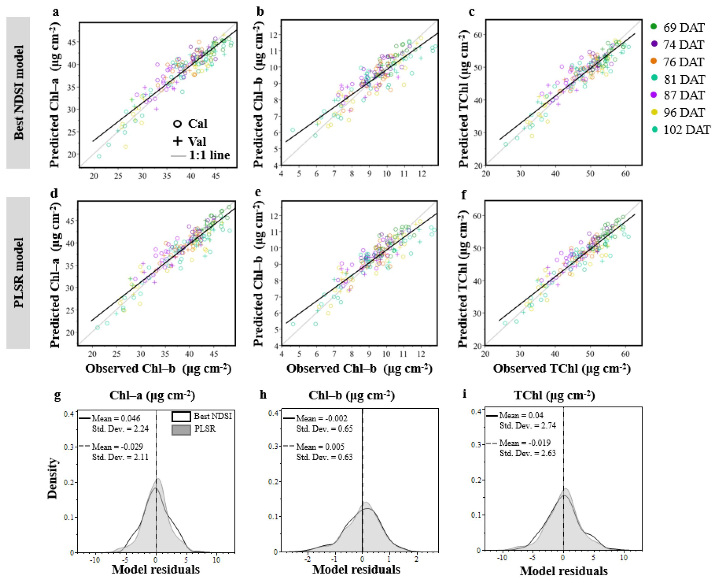
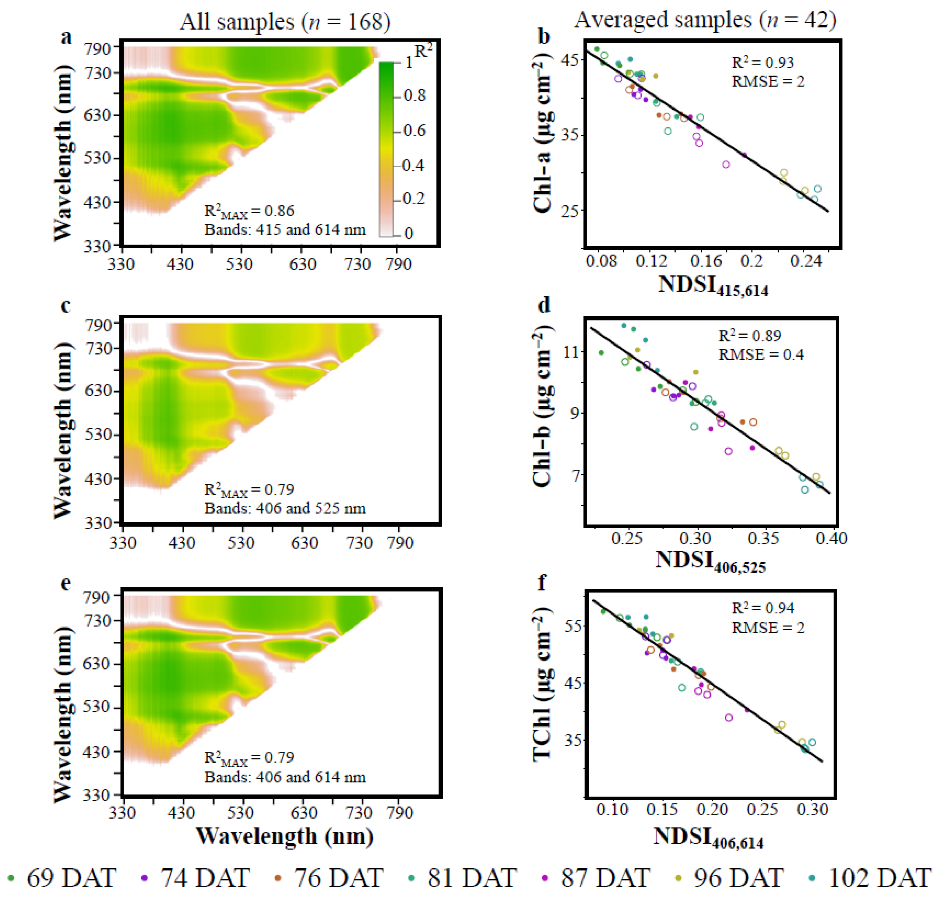
3.1. Vegetation Indices (VIs)

The R2 distribution of the two-band combinations to assess Chl-a, Chl-b and TChl content is presented in heat maps (Figure 3a,c,e). As expected, the heat maps were similar for the three chlorophyll parameters but with smaller areas with relatively high R2 values for Chl-b that is assumed to be the result of the smaller content of Chl-b in the leaves [54]. The selected bands for Chl-a and TChl are very similar, as can be expected since Chl-a is the major parameter in TChl. It is important to mention that bands adjacent to the selected ones will also show high R2 values (Table S5). The best two-band combination for the Chl-b estimation was 406 and 525 nm, supported by [55] reporting Chl-b absorption peaks in the blue and green regions. Analyzing the averaged spectral and destructive replicates per day (Figure 3b,d,f) resulted in bigger R2 values than the non-averaged ones (Figure 3a,c,e). All VIs were correlated to Chl-a, Chl-b and TChl and ranked based on R2 values (Supplementary Table S6). The top 10 performing VIs (Supplementary Table S6) used for Chl-a, Chl-b, and TChl estimation resulted in similar Cal and Val R2 as well as RMSE values (Table 1). The RMSE values (Figure 3 and Table 1) of indices developed in the current study are smaller than 10% of the active ranges of Chl-a, TChl and even of Chl-b. Previous studies, as detailed by Hallik et al. [56], presented smaller R2 and bigger RMSE values of Chl-a and Chl-b estimation based on spectral data and stated that studies estimating Chl-b used VIs that were more strongly correlated to Chl-a. In the current study, VIs were developed specifically for Chl-a as well as Chl-b estimation and are at the top in their category (Table 1). Banerjee et al. [24] developed a VI highly correlating with Chl-a, Chl-b and TChl concentrations based on wheat canopy side view imagery, acquired in a semi-controlled indoor environment. This VI used spectral regions related to nitrogen (1654 nm) and chlorophyll (727 nm). Sonobe et al. [29] applied spectral methods to estimate leaf Chl-a and Chl-b in wasabi grown in a semi-controlled environment indoors and resulted in RMSE values similar to the values achieved in the current study (Table 1). The current study presented improvement (in terms of R2 and RMSE) in the ability to estimate leaf Chl-a, Chl-b and TChl content values in wheat grown under field conditions and used the spectrally estimated values to calculate Chl-a/b (Figure 4). Spectral estimation of Chl-a/b was rarely published, Sonobe et al. [29] directly estimated Chl-a/b by spectral means resulting in RMSE values ranging from 0.13 to 0.6. In the current study, the RMSE can fit five to six times in the range of measured Chl-a/b values (Figure 4a). In the current study, the best VI for Chl-a estimation and the best VI for Chl-b estimation were used, and the ratio of the assessed values was calculated to obtain the Chl-a/b ratio. To the best of our knowledge, this approach of spectrally estimating Chl-a and Chl-b values in in vivo wheat leaves to calculate Chl-a/b has not yet been published. The VIs developed in the current study were using two or a few spectral bands, while the PLSR applied hundreds of spectral bands to estimate Chl-a and Chl-b values.

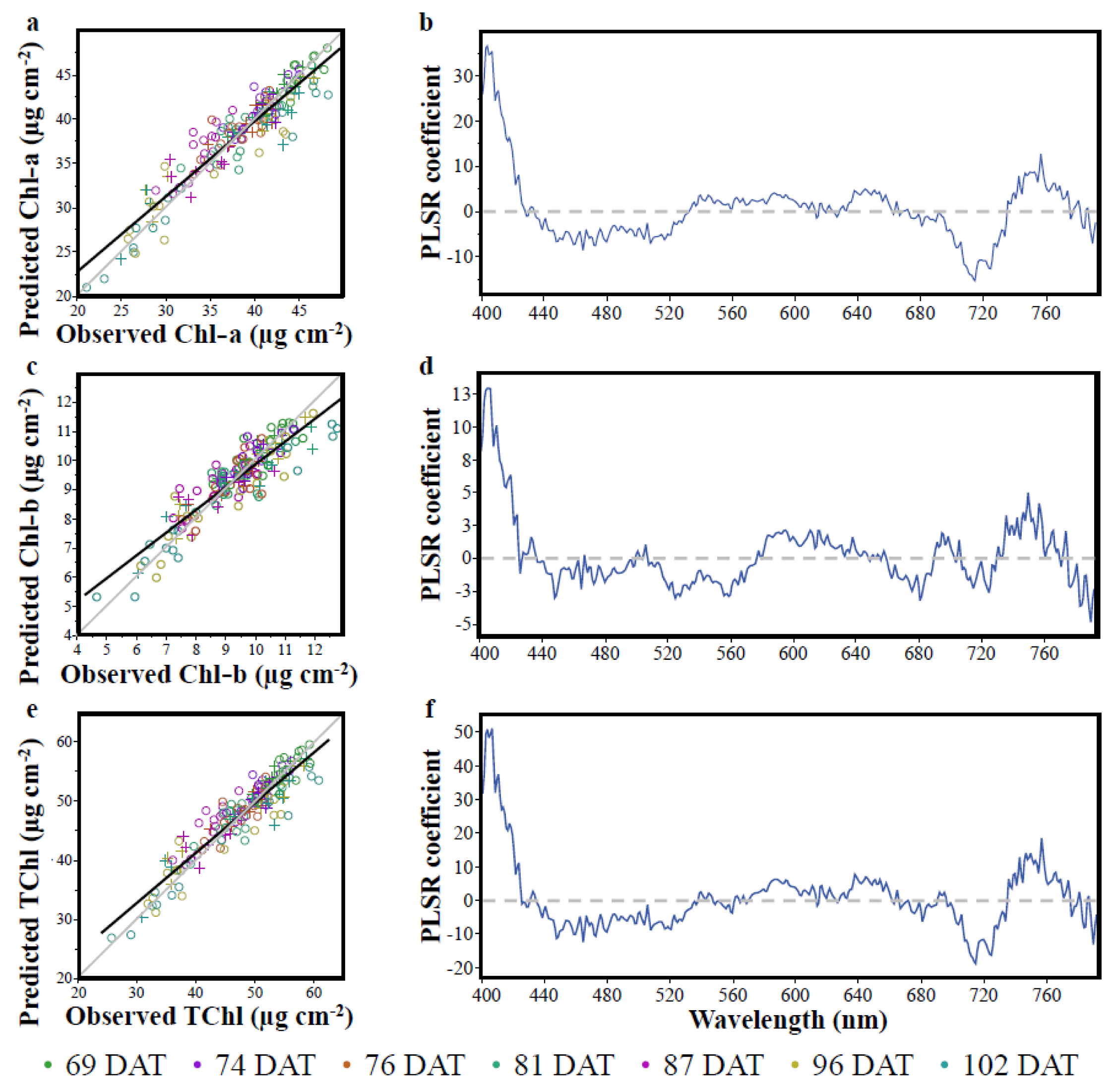
3.2. The Partial Least Squares Regression (PLSR)

The RMSE obtained for the estimated Chl-a, Chl-b and TChl concentrations by PLSR models (Table 2) are small enough to fit 12, 14, and 11 times, respectively, in the observed range of concentrations (Figure 5a,c,e). The estimation quality by PLSR and VIs (Table 1) in terms of R2 and RMSE was similar [57] for each of the chlorophylls. The VIs based on two to a few spectral bands and the PSLR based on 391 spectral bands resulted similarly, showing no advantage to either of them. The PLSR coefficients of the models (Figure 5b,d,f) are all showing the importance of the shortest wavelengths in agreement with the 406 and 415 nm wavelengths selected by the NDSIs (Figure 3a,c,e). The combined effect of the Chl-a and Chl-b coefficients can be seen in the TChl coefficients in the enhancement in the shortest wavelengths as well as the contradicting trends between 500 and 550 nm as well as around 700 nm. These insights support the stability of the models to be able to assess Chl-a and Chl-b and their sum as well as the ability to obtain Chl-a/b estimation (Figure 6). The Chl-a/b estimation based on the PLSR models (Figure 6) is showing improved R2 and RMSE in comparison to the VIs for the Val data set (Figure 4a) as well as for the averaged samples (Figure 4b), as was done for the VIs (Figure 3b,d,f). As expected, the averaged sample data resulted in the smallest RMSE value. The NDSI results (Figure 3a,c,e) support using the spectral range of 400 to 790 nm for the PLSR analysis. The observed vs. predicted chlorophyll parameter values are showing the same trend (above or below the trend line) for each of the two modeling methods: NDSIs and PLSR (Figure 7a–f). The distributions of residuals for each of the chlorophylls compared between the NDSI and PLSR models are not different (Figure 7g–i).

4. Conclusions

The current study aimed to spectrally assess Chl-a and Chl-b to identify the best VI or VIs for indirectly estimating Chl-a/b in three wild emmer wheat ILs. While there were no significant differences in Chl-a/b values between WW and WL treatments, the active range of the measured or predicted Chl-a/b values were five to six times the RMSE values for the non-averaged samples. Thus, it was concluded that:
(i)
The new VIs that were developed in the current study resulted in highly accurate Chl-a and Chl-b estimation.
(ii)
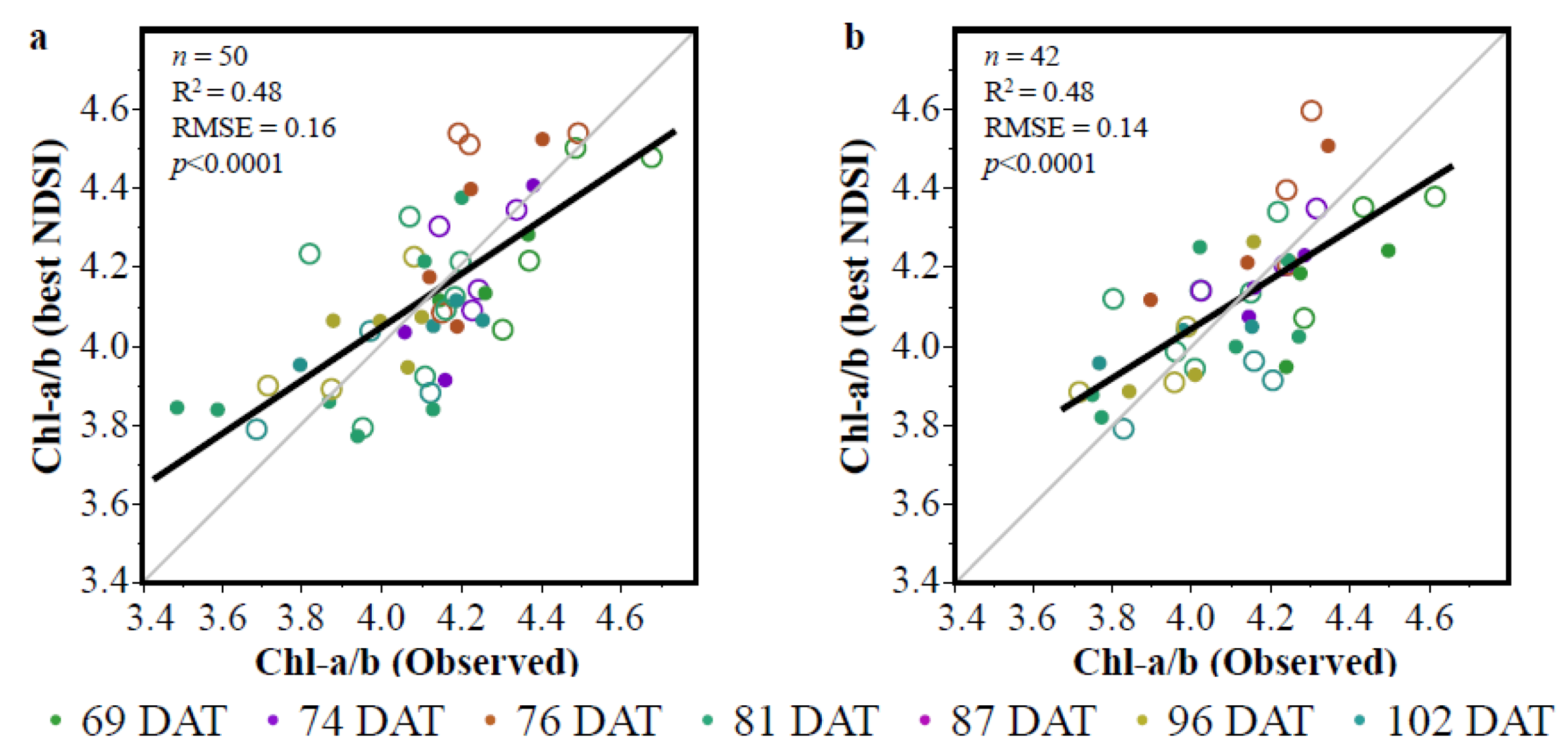
The developed VIs were able to indirectly estimate Chl-a/b.
(iii)
The VIs developed in the current study performed similarly to the PLSR.
The model quality achieved by VIs developed in the current study, in comparison to PLSR, supports sensors with a few spectral bands for practical use, while hyperspectral sensors are used for research to identify these spectral bands. The developed models should be tested in additional crops for breeding projects. Under more severe water stress scenarios, resulting in a wider range of Chl-a/b values, the models are expected to perform even better than in the current study. This concept of Chl-a and Chl-b direct estimation to indirectly assess Chl-a/b should be tested also for canopy-level spectral data collection. The current study presented a new approach, based on the spectral assessment of Chl-a and Chl-b for the non-destructive estimation of Chl-a/b, which can serve as a basis for future wheat breeding efforts as a non-destructive quick analysis method of pigments as a step towards canopy-level estimation. The ability to non-destructively assess Chl-a/b in vivo by spectral sensing will improve breeding efficiency toward developing climate-resilient wheat cultivars.

Supplementary Materials

The following supporting information can be downloaded at: https://www.mdpi.com/article/10.3390/rs14112585/s1. Table S2 references [58,59,60,61,62,63,64,65,66,67,68,69,70,71,72,73].

Author Contributions

Conceptualization, G.M., H.B., Z.P. and I.H.; Data curation, G.M.; Formal analysis, G.M. and U.K.; Funding acquisition, Z.P. and I.H.; Investigation, G.M., H.B., U.K. and I.H.; Methodology, G.M., H.B., U.K., Z.P. and I.H.; Project administration, I.H.; Resources, Z.P. and I.H.; Software, U.K.; Supervision, H.B., Z.P. and I.H.; Visualization, G.M.; Writing—original draft, G.M., H.B., U.K. and I.H.; Writing—review and editing, G.M., H.B., Z.P. and I.H. All authors have read and agreed to the published version of the manuscript.

Funding

This study was partially supported by the U.S. Agency for International Development Middle East Research and Cooperation (grant #M34-037), the Dutch Ministry of Foreign Affairs under Dutch development/foreign policy (Project WheatMAX), the Hebrew University of Jerusalem Intramural Research Fund Career Development, Hebrew University Center for Sustainability (OptiWheat), and the Hebrew University International School of Agricultural Sciences.

Data Availability Statement

Data available on request from the corresponding author.

Conflicts of Interest

The authors declare no conflict of interest.

References

  1. Myers, S.S.; Smith, M.R.; Guth, S.; Golden, C.D.; Vaitla, B.; Mueller, N.D.; Dangour, A.D.; Huybers, P. Climate change and global food systems: Potential impacts on food security and undernutrition. Annu. Rev. Public Health 2017, 38, 259–277. [Google Scholar] [CrossRef] [PubMed]
  2. Sade, N.; Peleg, Z. Future challenges for global food security under climate change. Plant Sci. 2020, 9–11. [Google Scholar] [CrossRef] [PubMed]
  3. Croft, H.; Chen, J.M.; Luo, X.; Bartlett, P.; Chen, B.; Staebler, R.M. Leaf chlorophyll content as a proxy for leaf photosynthetic capacity. Glob. Chang. Biol. 2017, 23, 3513–3524. [Google Scholar] [CrossRef] [PubMed]
  4. Croce, R.; Van Amerongen, H. Natural strategies for photosynthetic light harvesting. Nat. Chem. Biol. 2014, 10, 492–501. [Google Scholar] [CrossRef]
  5. Croft, H.; Chen, J.M. Leaf Pigment Content. Compr. Remote Sens. 2018, 117–142. [Google Scholar] [CrossRef]
  6. Lenaerts, B.; Collard, B.C.Y.; Demont, M. Review: Improving global food security through accelerated plant breeding. Plant Sci. 2019, 287, 110207. [Google Scholar] [CrossRef]
  7. Guo, Y.Y.; Yu, H.Y.; Kong, D.S.; Yan, F.; Zhang, Y.J. Effects of drought stress on growth and chlorophyll fluorescence of Lycium ruthenicum Murr. seedlings. Photosynthetica 2016, 54, 524–531. [Google Scholar] [CrossRef]
  8. Moran, R.; Porath, D. Chlorophyll determination in intact tissues using N,N -Dimethylformamide. Plant Physiol. 1980, 65, 478–479. [Google Scholar] [CrossRef] [Green Version]
  9. Wellburn, A.R. The Spectral determination of chlorophylls a and b, as well as total carotenoids, using various solvents with spectrophotometers of different resolution. J. Plant Physiol. 1994, 144, 307–313. [Google Scholar] [CrossRef]
  10. Gitelson, A.A.; Gritz, Y.; Merzlyak, M.N. Relationships between leaf chlorophyll content and spectral reflectance and algorithms for non-destructive chlorophyll assessment in higher plant leaves. J. Plant Physiol. 2003, 160, 271–282. [Google Scholar] [CrossRef]
  11. Gitelson, A.A.; Keydan, G.P.; Merzlyak, M.N. Three-band model for noninvasive estimation of chlorophyll, carotenoids, and anthocyanin contents in higher plant leaves. Geophys. Res. Lett. 2006, 33, 1–5. [Google Scholar] [CrossRef] [Green Version]
  12. Lopes, D.d.C.; Moura, L.d.O.; Steidle Neto, A.J.; Ferraz, L.d.C.L.; Carlos, L.d.A.; Martins, L.M. Spectral indices for non-destructive determination of lettuce pigments. Food Anal. Methods 2017, 10, 2807–2814. [Google Scholar] [CrossRef]
  13. Yamamoto, A.; Nakamura, T.; Adu-Gyamfi, J.J.; Saigusa, M. Relationship between chlorophyll content in leaves of sorghum and pigeonpea determined by extraction method and by chlorophyll meter (SPAD-502). J. Plant Nutr. 2002, 25, 2295–2301. [Google Scholar] [CrossRef]
  14. Joynson, R.; Molero, G.; Coombes, B.; Gardiner, L.J.; Rivera-Amado, C.; Piñera-Chávez, F.J.; Evans, J.R.; Furbank, R.T.; Reynolds, M.P.; Hall, A. Uncovering candidate genes involved in photosynthetic capacity using unexplored genetic variation in Spring Wheat. Plant Biotechnol. J. 2021, 19, 1537–1552. [Google Scholar] [CrossRef]
  15. Thenkabail, P.S.; Mariotto, I.; Gumma, M.K.; Middleton, E.M.; Landis, D.R.; Huemmrich, K.F. Selection of hyperspectral narrowbands (HNBs) and composition of hyperspectral two band vegetation indices (HVIs) for biophysical characterization and discrimination of crop types using field reflectance and Hyperion/EO-1 data. IEEE J. Sel. Top. Appl. Earth Obs. Remote Sens. 2013, 6, 427–439. [Google Scholar] [CrossRef] [Green Version]
  16. Casa, R.; Castaldi, F.; Pascucci, S.; Pignatti, S. Chlorophyll estimation in field crops: An assessment of handheld leaf meters and spectral reflectance measurements. J. Agric. Sci. 2015, 153, 876–890. [Google Scholar] [CrossRef]
  17. Pérez-Patricio, M.; Camas-Anzueto, J.L.; Sanchez-Alegría, A.; Aguilar-González, A.; Gutiérrez-Miceli, F.; Escobar-Gómez, E.; Voisin, Y.; Rios-Rojas, C.; Grajales-Coutiño, R. Optical method for estimating the chlorophyll contents in plant leaves. Sensors 2018, 18, 650. [Google Scholar] [CrossRef] [Green Version]
  18. Chappelle, E.W.; Kim, M.S.; McMurtrey, J.E. Ratio analysis of reflectance spectra (RARS): An algorithm for the remote estimation of the concentrations of chlorophyll A, chlorophyll B, and carotenoids in soybean leaves. Remote Sens. Environ. 1992, 39, 239–247. [Google Scholar] [CrossRef]
  19. Gitelson, A.A.; Viña, A.; Ciganda, V.; Rundquist, D.C.; Arkebauer, T.J. Remote estimation of canopy chlorophyll content in crops. Geophys. Res. Lett. 2005, 32, 1–4. [Google Scholar] [CrossRef] [Green Version]
  20. Yu, K.; Gnyp, M.L.; Gao, L.; Miao, Y.; Chen, X.; Bareth, G. Estimate leaf chlorophyll of rice using reflectance indices and partial least squares. Photogramm. Fernerkund. Geoinf. 2015, 2015, 45–54. [Google Scholar] [CrossRef]
  21. Gausman, H.W.; Allen, W.A. Optical parameters of leaves of 30 plant species. Plant Physiol. 1973, 52, 57–62. [Google Scholar] [CrossRef]
  22. Bannari, A.; Morin, D.; Bonn, F.; Huete, A.R. A review of vegetation indices. Remote Sens. Rev. 1995, 13, 95–120. [Google Scholar] [CrossRef]
  23. Giovos, R.; Tassopoulos, D.; Kalivas, D.; Lougkos, N.; Priovolou, A. Remote sensing vegetation indices in viticulture: A critical review. Agriculture 2021, 11, 457. [Google Scholar] [CrossRef]
  24. Banerjee, B.P.; Joshi, S.; Thoday-Kennedy, E.; Pasam, R.K.; Tibbits, J.; Hayden, M.; Spangenberg, G.; Kant, S. High-throughput phenotyping using digital and hyperspectral imaging-derived biomarkers for genotypic nitrogen response. J. Exp. Bot. 2020, 71, 4604–4615. [Google Scholar] [CrossRef] [Green Version]
  25. Bannari, A.; Khurshid, K.S.; Staenz, K.; Schwarz, J.W. A comparison of hyperspectral chlorophyll indices for wheat crop chlorophyll content estimation using laboratory reflectance measurements. IEEE Trans. Geosci. Remote Sens. 2007, 45, 3063–3074. [Google Scholar] [CrossRef]
  26. Chen, X.; Dong, Z.; Liu, J.; Wang, H.; Zhang, Y.; Chen, T.; Du, Y.; Shao, L.; Xie, J. Hyperspectral characteristics and quantitative analysis of leaf chlorophyll by reflectance spectroscopy based on a genetic algorithm in combination with partial least squares regression. Spectrochim. Acta Part A Mol. Biomol. Spectrosc. 2020, 243, 118786. [Google Scholar] [CrossRef]
  27. Gitelson, A.A. Nondestructive estimation of foliar pigment (chlorophylls, carotenoids, and anthocyanins) contents: Evaluating a semianalytical three-band model. In Hyperspectral Remote Sensing of Vegetation; Thenkabail, P.S., Lyon, J.G., Eds.; CRC: Boca Raton, FL, USA, 2011; pp. 141–165. [Google Scholar]
  28. Main, R.; Cho, M.A.; Mathieu, R.; O’Kennedy, M.M.; Ramoelo, A.; Koch, S. An investigation into robust spectral indices for leaf chlorophyll estimation. ISPRS J. Photogramm. Remote Sens. 2011, 66, 751–761. [Google Scholar] [CrossRef]
  29. Sonobe, R.; Yamashita, H.; Mihara, H.; Morita, A.; Ikka, T. Estimation of leaf chlorophyll a, b and carotenoid contents and their ratios using hyperspectral reflectance. Remote Sens. 2020, 12, 3265. [Google Scholar] [CrossRef]
  30. Ray, D.; Mueller, N.; West, P.; Foley, J. Yield trends are insufficient to double global crop production by 2050. PLoS ONE 2013, 8, e66428. [Google Scholar] [CrossRef] [Green Version]
  31. Abbo, S.; Pinhasi van-Oss, R.; Gopher, A.; Saranga, Y.; Ofner, I.; Peleg, Z. Plant domestication versus crop evolution: A conceptual framework for cereals and grain legumes. Trends Plant Sci. 2014, 19, 351–360. [Google Scholar] [CrossRef]
  32. Golan, G.; Hendel, E.; Méndez Espitia, G.E.; Schwartz, N.; Peleg, Z. Activation of seminal root primordia during wheat domestication reveals underlying mechanisms of plant resilience. Plant Cell Environ. 2018, 41, 755–766. [Google Scholar] [CrossRef] [PubMed]
  33. Bacher, H.; Zhu, F.; Gao, T.; Liu, K.; Dhatt, B.K.; Awada, T.; Zhang, C.; Distelfeld, A.; Yu, H.; Peleg, Z.; et al. Wild emmer introgression alters root-to-shoot growth dynamics in durum wheat in response to water stress. Plant Physiol. 2021, 187, 1149–1162. [Google Scholar] [CrossRef] [PubMed]
  34. Bacher, H.; Sharaby, Y.; Walia, H.; Peleg, Z. Modifying root-to-shoot ratio improves root water influxes in wheat under drought stress. J. Exp. Bot. 2022, 73, 1643–1654. [Google Scholar] [CrossRef] [PubMed]
  35. Peleg, Z.; Fahima, T.; Abbo, S.; Krugman, T.; Nevo, E.; Yakir, D.; Saranga, Y. Genetic diversity for drought resistance in wild emmer wheat and its ecogeographical associations. Plant Cell Environ. 2005, 28, 176–191. [Google Scholar] [CrossRef]
  36. Herrmann, I.; Karnieli, A.; Bonfil, D.J.; Cohen, Y.; Alchanatis, V. SWIR-based spectral indices for assessing nitrogen content in potato fields. Int. J. Remote Sens. 2010, 31, 5127–5143. [Google Scholar] [CrossRef]
  37. Inoue, Y.; Peñuelas, J.; Miyata, A.; Mano, M. Normalized difference spectral indices for estimating photosynthetic efficiency and capacity at a canopy scale derived from hyperspectral and CO2 flux measurements in rice. Remote Sens. Environ. 2008, 112, 156–172. [Google Scholar] [CrossRef]
  38. Singh, A.; Serbin, S.P.; McNeil, B.E.; Kingdon, C.C.; Townsend, P.A. Imaging spectroscopy algorithms for mapping canopy foliar chemical and morphological traits and their uncertainties. Ecol. Appl. 2015, 25, 2180–2197. [Google Scholar] [CrossRef] [Green Version]
  39. Wold, S.; Sjöström, M.; Eriksson, L. PLS-regression: A basic tool of chemometrics. Chemom. Intell. Lab. Syst. 2001, 58, 109–130. [Google Scholar] [CrossRef]
  40. Yang, G.; Liu, J.; Zhao, C.; Li, Z.; Huang, Y.; Yu, H.; Xu, B.; Yang, X.; Zhu, D.; Zhang, X.; et al. Unmanned aerial vehicle remote sensing for field-based crop phenotyping: Current status and perspectives. Front. Plant Sci. 2017, 8. [Google Scholar] [CrossRef]
  41. McKinney, W. Data structures for statistical computing in python. Proc. 9th Python Sci. Conf. 2010, 1, 56–61. [Google Scholar] [CrossRef] [Green Version]
  42. Virtanen, P.; Gommers, R.; Oliphant, T.E.; Haberland, M.; Reddy, T.; Cournapeau, D.; Burovski, E.; Peterson, P.; Weckesser, W.; Bright, J.; et al. SciPy 1.0: Fundamental algorithms for scientific computing in python. Nat. Methods 2020, 17, 261–272. [Google Scholar] [CrossRef] [Green Version]
  43. Pedregosa, F.; Grisel, O.; Weiss, R.; Passos, A.; Brucher, M.; Varoquax, G.; Gramfort, A.; Michel, V.; Thirion, B.; Grisel, O.; et al. Scikit-learn: Machine learning in python. J. Mach. Learn. Res. 2011, 12, 2825–2830. [Google Scholar]
  44. Ashraf, M.; Harris, P.J.C. Photosynthesis under stressful environments: An overview. Photosynthetica 2013, 51, 163–190. [Google Scholar] [CrossRef]
  45. Pyke, K.A.; Jellings, A.J.; Leech, R.M. Variation in mesophyll cell number and size in wheat leaves. Ann. Bot. 1990, 65, 679–683. [Google Scholar] [CrossRef]
  46. Guru, T.; Padma, V.; Reddy, D.V.V.; Rao, P.R.; Sanjeeva Rao, D.; Ramesh, T.; Radhakrishna, K.V. Natural variation of top three leaf traits and their association with grain yield in rice hybrids. Indian J. Plant Physiol. 2017, 22, 141–146. [Google Scholar] [CrossRef]
  47. Gitelson, A.A.; Merzlyak, M.N. Remote estimation of chlorophyll content in higher plant leaves. Int. J. Remote Sens. 1997, 18, 2691–2697. [Google Scholar] [CrossRef]
  48. Carter, G.A. Ratios of leaf reflectances in narrow wavebands as indicators of plant stress. Int. J. Remote Sens. 1994, 15, 517–520. [Google Scholar] [CrossRef]
  49. Zarco-Tejada, P.J.; Miller, J.R.; Noland, T.L.; Mohammed, G.H.; Sampson, P.H. Scaling-up and model inversion methods with narrowband optical indices for chlorophyll content estimation in closed forest canopies with hyperspectral data. IEEE Trans. Geosci. Remote Sens. 2001, 39, 1491–1507. [Google Scholar] [CrossRef] [Green Version]
  50. Barnes, E.M.; Clarke, T.R.; Richards, S.E. Coincident detection of crop water stress, nitrogen status and canopy density using ground-based multispectral data. In Proceedings of the Fifth International Conference on Precision Agriculture, Bloomington, MN, USA, 16–19 July 2000; Robert, P.C., Rust, R.H., Larson, W.E., Eds.; American Society of Agronomy: Madison, WI, USA, 2000. [Google Scholar]
  51. Guyot, G.; Baret, F.; Major, D.J. High spectral resolution: Determination of spectral shifts between the red and infrared. Int. Arch. Photogramm. Remote Sens. 1988, 11, 750–760. [Google Scholar] [CrossRef]
  52. Raymond Hunt, E.; Daughtry, C.S.T.; Eitel, J.U.H.; Long, D.S. Remote sensing leaf chlorophyll content using a visible band index. Agron. J. 2011, 103, 1090–1099. [Google Scholar] [CrossRef] [Green Version]
  53. Haboudane, D.; Miller, J.R.; Tremblay, N.; Zarco-Tejada, P.J.; Dextraze, L. Integrated narrow-band vegetation indices for prediction of crop chlorophyll content for application to precision agriculture. Remote Sens. Environ. 2002, 81, 416–426. [Google Scholar] [CrossRef]
  54. Datt, B. Remote sensing of chlorophyll a, chlorophyll b, chlorophyll a+b, and total carotenoid content in eucalyptus leaves. Remote Sens. Environ. 1998, 66, 111–121. [Google Scholar] [CrossRef]
  55. Ustin, S.L.; Jacquemoud, S. How the optical properties of leaves modify the absorption and scattering of energy and enhance leaf functionality. In Remote Sensing of Plant Biodiversity; Cavender-Bares, J., Gamon, J.A., Townsend, P.A., Eds.; Springer International Publishing: Cham, Switzerland, 2020; pp. 349–384. ISBN 9783030331573. [Google Scholar]
  56. Hallik, L.; Kazantsev, T.; Kuusk, A.; Galmés, J.; Tomás, M.; Niinemets, Ü. Generality of relationships between leaf pigment contents and spectral vegetation indices in Mallorca (Spain). Reg. Environ. Chang. 2017, 17, 2097–2109. [Google Scholar] [CrossRef]
  57. Herrmann, I.; Pimstein, A.; Karnieli, A.; Cohen, Y.; Alchanatis, V.; Bonfil, D.J. LAI assessment of wheat and potato crops by VENμS and Sentinel-2 bands. Remote Sens. Environ. 2011, 115, 2141–2151. [Google Scholar] [CrossRef]
  58. Rouse, J.W.; Haas, R.H.; Schell, J.A.; Deering, D.W.; Harlan, J.C. Monitoring the Vernal Advancement and Retrogradation (Green Wave Effect) of Natural Vegetation; Texas A&M University Remote Sensing Center: College Station, TX, USA, 1974. [Google Scholar]
  59. Jordan, C.F. Derivation of Leaf-Area Index from Quality of Light on the Forest Floor. Ecology 1969, 50, 663–666. [Google Scholar] [CrossRef]
  60. Rondeaux, G.; Steven, M.; Baret, F. Optimization of Soil-Adjusted Vegetation Indices. Remote Sens. Environ. 1996, 55, 95–107. [Google Scholar] [CrossRef]
  61. Smith, R.; Adams, J.; Stephens, D.; Hick, P. Forecasting Wheat Yield in a Mediterranean-Type Environment from the NOAA Satellite. Crop Pasture Sci. 1995, 46, 113–125. [Google Scholar] [CrossRef]
  62. Daughtry, C.S.T.; Walthall, C.L.; Kim, M.S.; Brown de Colostoun, E.; McMurtrey, J.E. Estimating Corn Leaf Chlorophyll Concentration from Leaf and Canopy Reflectance. Remote Sens. Environ. 2000, 74, 229–239. [Google Scholar] [CrossRef]
  63. Broge, N.H.; Leblanc, E. Comparing Prediction Power and Stability of Broadband and Hyperspectral Vegetation Indices for Estimation of Green Leaf Area Index and Canopy Chlorophyll Density. Remote Sens. Environ. 2001, 76, 156–172. [Google Scholar] [CrossRef]
  64. Peñuelas, J.; Filella, I. Reflectance Assessment of Mite Effects on Apple Trees. Int. J. Remote Sens. 1995, 16, 2727–2733. [Google Scholar] [CrossRef]
  65. Barnes, J.D.; Balaguer, L.; Manrique, E.; Elvira, S.; Davison, A.W. A Reappraisal of the Use of DMSO for the Extraction and Determination of Chlorophylls a and b in Lichens and Higher Plants. Environ. Exp. Bot. 1992, 32, 85–100. [Google Scholar] [CrossRef]
  66. Gamon, J.A.; Penuelas, J.; Field, C.B. A Narrow-Waveband Spectral Index That Tracks Diurnal Changes in Photosynthetic Efficiency. Remote Sens. Environ. 1992, 41, 35–44. [Google Scholar] [CrossRef]
  67. Peñuelas, J.; Gamon, J.A.; Fredeen, A.L.; Merino, J.; Field, C.B. Reflectance Indices Associated with Physiological Changes in Nitrogen- and Water-Limited Sunflower Leaves. Remote Sens. Environ. 1994, 48, 135–146. [Google Scholar] [CrossRef]
  68. Lichtenthaler, H.K. The Stress Concept in Plants: An Introduction. Plant Physiol. Biochem. 1996, 148, 4–14. [Google Scholar] [CrossRef]
  69. Penuelas, J.; Baret, F.; Filella, I. Semi-Empirical Indices to Assess Carotenoids/Chlorophyll a Ratio from Leaf Spectral Reflectance. Photosynthetica 1995, 31, 221–230. [Google Scholar]
  70. Gitelson, A.A.; Merzlyak, M.N.; Chivkunova, O.B. Optical Properties and Nondestructive Estimation of Anthocyanin Content in Plant Leaves. Photochem. Photobiol. 2001, 74, 38. [Google Scholar] [CrossRef]
  71. Gitelson, A.A.; Zur, Y.; Chivkunova, O.B.; Merzlyak, M.N. Assessing Carotenoid Content in Plant Leaves with Reflectance Spectroscopy. Photochem. Photobiol. 2002, 75, 272. [Google Scholar] [CrossRef]
  72. Roujean, J.L.; Breon, F.M. Estimating PAR Absorbed by Vegetation from Bidirectional Reflectance Measurements. Remote Sens. Environ. 1995, 51, 375–384. [Google Scholar] [CrossRef]
  73. Merzlyak, M.N.; Gitelson, A.A.; Chivkunova, O.B.; Rakitin, V.Y. Non-Destructive Optical Detection of Pigment Changes during Leaf Senescence and Fruit Ripening. Physiol. Plant. 1999, 106, 135–141. [Google Scholar] [CrossRef] [Green Version]
Figure 1. The experimental site, the plastic-covered net house (a). Before planting (b). Wheat plants grown in the net house, the relevant plants are on the 3rd row from the left (c).
Remotesensing 14 02585 g001
Figure 2. Chlorophyll concentrations and flag leaf reflectance spectra of randomly selected leaf samples in five dates throughout the season (one leaf per date). Barplot of varying concentrations of total chlorophyll (TChl), chlorophyll a (Chl-a) and chlorophyll b (Chl-b) (a). Corresponding reflectance spectra of each sample chlorophyll concentration (b). Colors represents chlorophyll concentrations and their respective reflectance spectrum.
Remotesensing 14 02585 g002
Figure 3. All possible two-band combinations by normalized difference vegetation index (NDSI) heat maps R2 values (p < 0.0001) for regression with Chl-a, Chl-b, and TChl content on all 168 samples (a,c,e). Linear regression of Chl-a, Chl-b, and TCh content on all 168 samples (a,c,e). Linear regression of Chl-a, Chl-b, and TChl (n = 42) with their corresponding highest-ranking NDSI based on averaged NDSI values per genotype, irrigation regime and DAT (b,d,f). The black lines are the trend line. Chl-a (a,b), Chl-b (c,d), and TChl (e,f). Hollow and filled dots stand for water-limited (WL) and well-watered (WW), respectively. RMSE stands for root mean square error; DAT stands for days after transplant.
Remotesensing 14 02585 g003
Figure 4. Quality of Chl-a/b spectral estimation by normalized difference spectral index (NDSI). The Chl-a/b (observed) data were acquired by extraction of Chl-a and Chl-b. The Chl-a/b (best NDSI) data were calculated by applying the top (NDSI estimating Chl-a and Chl-b (Table 1). The Val data set is presented in Table 1 (a). Averaged values per genotype, irrigation regime and DAT as presented in Figure 3b,d,f (b). DAT stands for days after transplant. Hollow and filled dots stand for water-limited (WL) and well-watered (WW), respectively; the black lines are the trend lines and the gray lines are the 1:1 lines.
Remotesensing 14 02585 g004
Figure 5. Chl-a, Chl-b, and TChl content estimation by partial least squares (PLSR) models. Observed vs. predicted chlorophyll values (a,c,e). Solid black lines are calibration (Cal) best-fit lines and 1:1 lines are gray. Circle and Plus markers represent Cal and Val samples, respectively. The PLSR coefficients for each of the models (b,d,f), solid blue lines are coefficient values and dashed gray lines are the zero-coefficient value. Chl-a (a,b), Chl-b (c,d), and TChl (e,f).
Remotesensing 14 02585 g005
Figure 6. Quality of Chl-a/b spectral estimation. The Chl-a/b (observed) data were acquired by extraction of Chl-a and Chl-b. The Chl-a/b (best PLSR) data were calculated by applying the PLSR models estimating Chl-a and Chl-b (Table 2). The Val data set is presented in Table 2. Hollow and filled dots stand for water-limited (WL) and well-watered (WW), respectively (a). Averaged values per genotype, irrigation regime and DAT, as presented in Figure 5b,d,f (b). The black lines are the trend lines and the gray lines are the 1:1 lines. Hollow and filled dots stand for WL and WW, respectively.
Remotesensing 14 02585 g006
Figure 7. Chlorophyll a (Chl-a), chlorophyll b (Chl-b), and total chlorophyll T(Chl) content estimation by their respective best normalized difference spectral index (NDSI) model and partial least square regression (PLSR) model. Best NDSIs predicted chlorophyll values (ac); PLSR predicted vs. observed chlorophyll values (df). Solid black lines are best-fit lines, and circle and plus markers represent calibration (Cal) and validation (Val) samples, respectively. DAT stands for days after transplant. Kernel density plot of residuals (gi) comparing the best NDSI and PLSR models for predicting chlorophyll content. Black lines represent mean value of residuals from NDSI model, while dashed grey lines represent mean value of residual from PLSR model. Student t-test of the residuals shows no significant differences between the two models across all chlorophyll content at 0.05 alpha level.
Remotesensing 14 02585 g007
Table 1. The top ten predictions for Chl-a, Chl-b, and TChl are presented based on all 33 VIs, NDSI-generated VIs from the leaf reflectance spectra by the PolyPen sensor.
Ranking 1VICal R2RMSEPC (μg cm−2)% RMSEPCVal R2RMSEPV (μg cm−2)% RMSEPVReferences
Chl-a (n = 118) (n = 50)
1NDSI415,6140.852.348.540.872.029.24Current study
2ZMI0.822.529.300.802.4711.31[49]
3CIred-edge0.822.549.370.812.4311.10[19]
4Carter 10.822.579.450.822.3810.89[48]
5CIgreen0.812.619.600.832.2810.42[19]
6GM10.812.629.640.832.2810.43[47]
7GM20.822.579.460.802.4811.37[47]
8NDRE0.812.629.660.802.4711.31[50]
9REIP0.802.719.970.812.4411.15[51]
10TGI0.782.8110.350.802.5111.49[52]
Chl-b (n = 117) (n = 50)
1NDSI406,5250.780.738.470.820.569.59Current study
2Carter 10.670.8810.860.560.7913.49[48]
3TGI0.640.9011.150.630.7612.90[52]
4GM10.640.9011.100.630.7713.16[47]
5CIgreen0.630.9111.250.620.7813.22[19]
6TCARI0.620.9211.370.610.7813.26[53]
7Datt10.600.9511.710.560.8514.42[54]
8REIP0.590.9611.840.540.8414.30[51]
9MCARI0.590.9611.840.540.8414.34[53]
10NDRE0.580.9711.840.550.8514.45[50]
TChl (n = 116) (n = 50)
1NDSI406,6140.862.828.030.872.519.08Current study
2GM1/Carter 10.852.918.300.852.619.42Current study
3GM1-Carter 10.833.058.700.842.689.69Current study
4Carter 10.803.309.420.793.0711.09[48]
5GM10.793.389.630.812.9410.63[47]
6CIgreen0.793.399.660.812.9510.65[19]
7ZMI0.793.409.680.773.2811.84[49]
8CIred-edge0.793.429.760.773.2211.65[19]
9GM20.793.449.810.763.3111.95[47]
10TGI0.773.5510.120.783.1411.34[52]
All R2 values are significant to p < 0.0001. 1 Based on R2 of all samples (Supplementary Table S6).
Table 2. The Chl-a, Chl-b, and TChl estimation based on PLSR model.
ChlorophyllCal R2RMSEPC
(μg cm−2)
% RMSEPCVal R2RMSEPV
(μg cm−2)
% RMSEPV
Chl-a0.882.117.760.862.089.52
Chl-b0.800.668.100.810.579.63
TChl0.872.687.630.862.519.05
Publisher’s Note: MDPI stays neutral with regard to jurisdictional claims in published maps and institutional affiliations.

