Article

Three-Dimensional Distribution of Biomass Burning Aerosols from Australian Wildfires Observed by TROPOMI Satellite Observations

1
Univ Paris Est Creteil and Université Paris Cité, CNRS, LISA, 94010 Créteil, France
2
ARIA Technologies, 92100 Boulogne-Billancourt, France
3
Université Paris Cité and Univ Paris Est Creteil, CNRS, LISA, 75013 Paris, France
4
Istituto Nazionale di Geofisica e Vulcanologia, Osservatorio Etneo, 95123 Catania, Italy
5
LATMOS/IPSL, Sorbonne Université, UVSQ, CNRS, 75252 Paris, France
6
LMD, Sorbonne Universités, CNRS, 75231 Paris, France
7
Center for Astrophysics, Harvard & Smithsonian, Cambridge, MA 02138, USA
8
School of Natural Sciences, Minerva University, San Francisco, CA 94103, USA
9
German Aerospace Center (DLR), Remote Sensing Technology Institute, Oberpfaffenhofen, 82234 Weßling, Germany
*
Author to whom correspondence should be addressed.
Remote Sens. 2022, 14(11), 2582; https://doi.org/10.3390/rs14112582
Submission received: 21 April 2022 / Revised: 14 May 2022 / Accepted: 20 May 2022 / Published: 27 May 2022
(This article belongs to the Special Issue Advances in Remote Sensing of Biomass Burning)

Abstract

:
We present a novel passive satellite remote sensing approach for observing the three-dimensional distribution of aerosols emitted from wildfires. This method, called AEROS5P, retrieves vertical profiles of aerosol extinction from cloud-free measurements of the TROPOMI satellite sensor onboard the Sentinel 5 Precursor mission. It uses a Tikhonov–Phillips regularization, which iteratively fits near-infrared and visible selected reflectances to simultaneously adjust the vertical distribution and abundance of aerosols. The information on the altitude of the aerosol layers is provided by TROPOMI measurements of the reflectance spectra at the oxygen A-band near 760 nm. In the present paper, we use this new approach for observing the daily evolution of the three-dimensional distribution of biomass burning aerosols emitted by Australian wildfires on 20–24 December 2019. Aerosol optical depths (AOD) derived by vertical integration of the aerosol extinction profiles retrieved by AEROS5P are compared with MODIS, VIIRS and AERONET coincident observations. They show a good agreement in the horizontal distribution of biomass burning aerosols, with a correlation coefficient of 0.87 and a mean absolute error of 0.2 with respect to VIIRS. Moderately lower correlations (0.63) were found between AODs from AEROS5P and MODIS, while the range of values for this comparison was less than half of that with respect to VIIRS. A fair agreement was found between coincident transects of vertical profiles of biomass burning aerosols derived from AEROS5P and from the CALIOP spaceborne lidar. The mean altitudes of these aerosols derived from these two measurements showed a good agreement, with a small mean bias (185 m) and a correlation coefficient of 0.83. Moreover, AEROS5P observations reveal the height of injection of the biomass burning aerosols in 3D. The highest injection heights during the period of analysis were coincident with the largest fire radiative power derived from MODIS. Consistency was also found with respect to the vertical stability of the atmosphere. The AEROS5P approach provides retrievals for cloud-free scenes over several regions, although currently limited to situations with a dominating presence of smoke particles. Future developments will also aim at observing other aerosol species.

Graphical Abstract

1. Introduction

Biomass burning (BB) aerosols have a major impact on the environment. Large-scale emissions of these particles have large impacts on the radiation balance and climate. Fresh and aged biomass burning plumes produce diabatic radiative heating, e.g., [1], and then can lead to self-lofting of the plume, e.g., [2]. They can produce a warming or cooling radiative forcing, depending on their optical properties and then their atmospheric lifetime [3]. If vertically and horizontally co-located with clouds, they may modify their properties and precipitation by acting as cloud condensation nuclei, e.g., [4], depending on the age and the composition of the particles, e.g., [5]. When transported near the surface, BB aerosols degrade air quality and cause negative long-term health effects, e.g., [6]. The characterization of BB aerosols and their environmental impacts is hampered by the large spatiotemporal variability of wildfires and the difficulty to predict their occurrence and intensity.
The altitudes at which BB aerosol plumes are injected into the atmosphere during emission by wildfires is also important for the estimation of their impacts, and is very uncertain. Chemistry-transport models often predict them using semi-empirical methods based on satellite measurements of fire radiative power, burned surface areas, fire temperature, etc.; e.g., [7,8]. The limitations of these methods are shown by comparisons with observations of the fire plumes [9,10]. Their uncertainties are linked to the lack of sufficient knowledge on the characteristics of the fires, pyro-convection processes, their effects on atmospheric stability and feedback. Accurate knowledge on the smoke injection heights is important for studying the regions that these particles may reach and thus their impacts. This is linked to the fact that horizontal transport strongly varies depending on the altitude of the atmospheric layers.
A description of both the horizontal and vertical distributions of atmospheric constituents within BB plumes is required to study their evolution in time and space and their impacts on the environment. Passive remote sensing allows the observation of the abundance of several atmospheric gaseous species, such as ozone or water vapor, in terms of vertical profiles. This is done by using the dependence of the spectral absorption signatures of these gases with respect to their vertical distribution. On the other hand, classic approaches of aerosol passive remote sensing, using sensors such as MODIS (Moderate Resolution Imaging Spectroradiometer), have provided for several decades’ total atmospheric columns of aerosol optical depth (AOD), which only describe their horizontal distributions. This is partly linked to the fact that the spectral signature of aerosols only depends on their altitude for specific parts of the radiation spectrum, such as the oxygen absorption bands in the near infrared, e.g., [11], and the thermal infrared but only for coarse particles such as desert dust, e.g., [12]. Indeed, extinction efficiencies of fine particles much smaller than the wavelengths of thermal radiation are mostly very low and thus their signature in this spectral domain is mainly negligeable. This is the case for most fine particles such as soot aerosols emitted by fires, for which thermal infrared extinction coefficients are at least a factor of ~20 smaller than in the visible [13].
Satellite high spectral resolution measurements in the near infrared, with strong spectral signatures of both fine and coarse aerosols, are only performed by a few spaceborne sensors, such as Global Ozone Monitoring Experiment-2 (GOME-2) [14] and TROPospheric Ozone Monitoring Instrument (TROPOMI) [15], respectively onboard MetOp-A/B/C since 2007 and Sentinel 5 Precursor (S5P) since 2017. Their analysis is challenging since the interactions between radiation and aerosols simultaneously depend on their abundance, altitude, size distribution [16] and composition [17]. Another difficulty for observing aerosols from space comes from the fact that the composition and thermodynamic state of the atmosphere are constantly evolving, and so are the optical properties of aerosols [18,19], which hampers tracing of the path of aerosol plumes in the atmosphere.
Several approaches allow the observation of the vertical profiles of particulate matter in the atmosphere. Airborne in situ sensors provide direct and accurate measurements of aerosol vertical profiles [20], but their availability is limited in space and time as they are mainly performed during field campaigns. Active remote sensing based on lidar instruments like the CALIOP lidar onboard the Cloud-Aerosol Lidar and Infrared Pathfinder Satellite Observation (CALIPSO) satellite can retrieve latitudinal transects of aerosol vertical profiles [21] but only for a very narrow field of view (90 m wide footprints). On a given day, these measurements are spaced longitudinally by about ~2000 km at mid-latitudes (for either daytime or nighttime overpasses). Recently, passive remote sensing of the reflectance spectrum of the oxygen absorption A-band has allowed the retrieval of mean aerosol heights over dark targets, from GOME-2 [11,21] and TROPOMI [22,23] measurements with horizontal resolutions of respectively 40 km × 80 km and 3.5 km × 5.5 km. Using nine viewing angles, aerosol mean heights are also derived from the Multi Angle Imaging Spectroradiometer (MISR) [24] on bright and dark surfaces at 4.4 km horizontal resolution [25,26]. The vertical profile of desert dust coarse particles is retrieved from space using measurements of the thermal infrared spectrum from the Infrared Atmospheric Sounding Interferometer (IASI) instrument [12,27,28,29]. The latter observations are horizontally spaced by 25 km (at the nadir), so that they allow the observation of the 3D distribution of coarse particles having a strong radiative signature in the thermal infrared (such as desert dust). This may also be found for fine particles in some specific cases, due to the presence of significant absorption bands in the thermal infrared, as seen for sulfuric acid and ammonium sulfate [30], or for highly abundant aerosols emitted by large-scale outbreaks, e.g., [31]. However, this is not the case for most fine particles such as those originating from fires and most urban pollution, e.g. [13].
In this paper, we present a new approach called AEROS5P for observing the 3D distribution of BB fine aerosols based on TROPOMI measurements. This method derives vertical profiles of aerosol extinction at 550 nm (linearly interpolated between 496 and 673 nm) for cloud-free pixels of TROPOMI. AEROS5P thus provides the daily observation of the full 3D distribution of fine BB particles, for cloud-free conditions. The determination of the vertical profile of aerosol extinction from passive spectral measurements is based on a Tikhonov–Philips-like auto-adaptive regularization. This technique was originally developed for desert dust aerosols and IASI measurements [12], lately applied also to volcanic sulphate aerosol [32], but it is here adapted for BB particles and TROPOMI data. For simultaneously constraining the aerosol vertical distribution and AOD, the method uses both near infrared and visible spectra from TROPOMI (instrument details are given in Section 2). The vertical profiles of BB aerosols derived from AEROS5P can also be used to calculate AODs and mean aerosol layer heights.
We use AEROS5P for describing the 3D distribution of BB aerosols emitted during the extreme large-scale wildfires that occurred in Australia in late 2019 and the beginning of 2020. Our approach provides an unprecedented 3D description of the smoke injection height and transport pathways. We mainly focus on the period of 20–24 December 2019, which is particularly characterized by cloud-free conditions over most of the Australian continent during several days. The record-breaking Australian fires [33] caused a catastrophic impact on the economy, the population health, and biodiversity [34]. Massive amounts of smoke were injected into the upper troposphere and the stratosphere. The subsequent in-plume radiative heating contributed to the formation of a smoke-charged confined ascending vortex that reached 35 km of altitude [2]. The plumes were transported very long distances and dominated the stratospheric aerosol layer of the whole Southern Hemisphere for several months, producing the most important impact on the climate system linked to stratospheric aerosol perturbations since the eruption of Pinatubo in 1991 [3].
This paper provides a description of the AEROS5P algorithm backbone, and all additional datasets used in this work (Section 2). Section 3 shows comparisons of AEROS5P retrievals with respect to observations of the AOD from AERONET network stations, its horizontal distribution from MODIS and VIIRS (Visible Infrared Imaging Radiometer Suite) and vertical profiles derived from the CALIOP spaceborne lidar. The following section describes the 3D distribution of smoke plumes and their injection heights for the period of analysis, and the link with respect to the wildfire activity and meteorological conditions. Section 5 draws conclusions and discusses perspectives of this work.

2. Materials and Methods

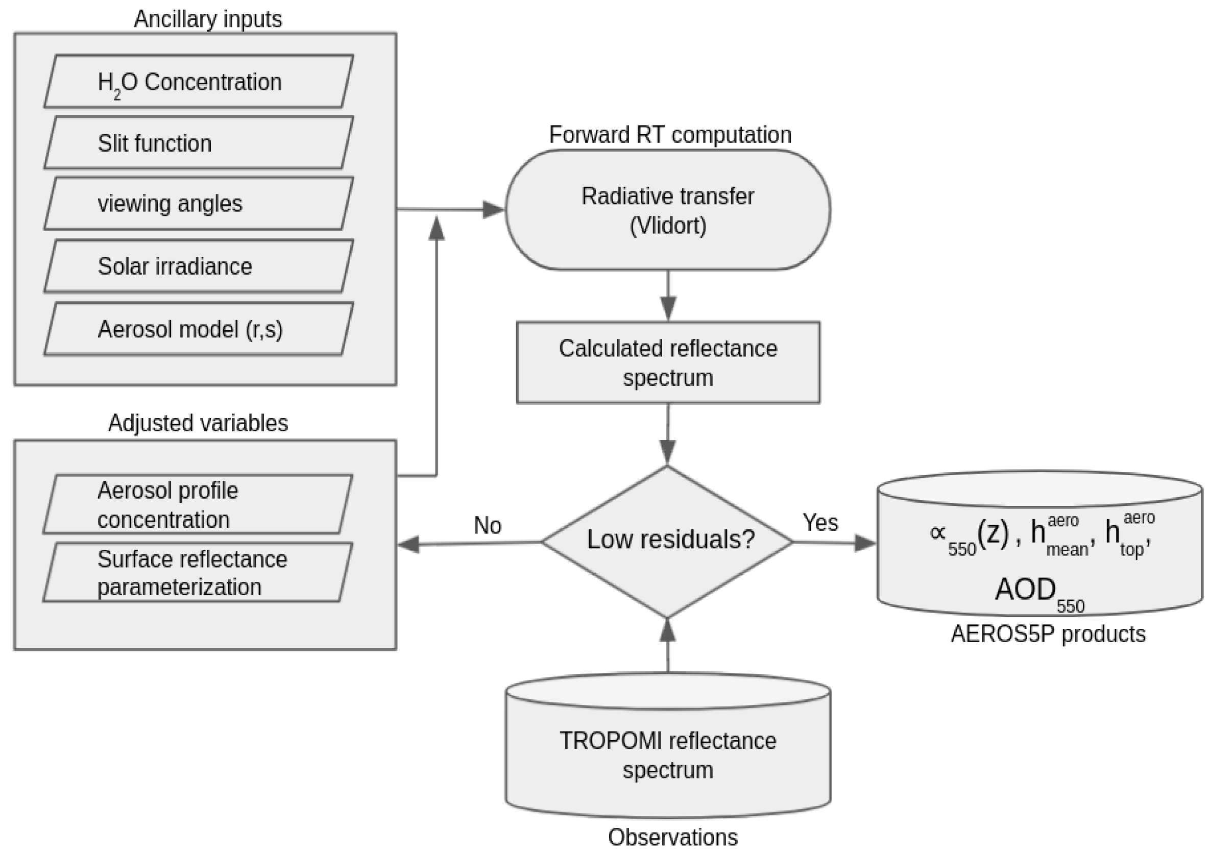
2.1. The AEROS5P Method

An overview scheme of the AEROS5P algorithm is presented in Figure 1. The approach simulates radiative transfer in the surface–atmosphere system and calculates reflectance spectra in the visible and near infrared. The simulated reflectances are then compared with those measured by TROPOMI. The retrieval algorithm estimates the vertical profile of aerosol content in the atmosphere with a regularized iterative process, as done for the profiles of desert dust by [12,27,35] and ozone by, e.g., [36,37]. As typically done in the Tikhonov–Philips regularization [35] and the optimal estimation method [38], the cost function that is minimized is the sum of the residuals of the measurement vector and the difference between the state vector and a priori values. These last ones are weighted by respectively radiometric noise and the regularization constraint (as described in [35]).
In absence of clouds, the spectral signature at the oxygen A-band near 760 nm provides information on the altitude of aerosols, e.g., [39]. This is explained by the fact that the effective depth of the layer of oxygen absorbing radiation depends on the altitude of aerosols. When scattering particles are located at higher (lower) atmospheric layers, solar radiation penetrates less close (closer) to the surface and thus less (more) oxygen molecules absorb radiation. On the other hand, the other visible TROPOMI measurements used by AEROS5P do not depend on the altitude of aerosols and thus are jointly employed for deriving their abundance in terms of AOD.
The final products of AEROS5P are vertical profiles of aerosol extinction at 550 nm (α550), aerosol top layer height (htop), mean aerosol height (hmean) and AODs for cloud-free TROPOMI pixels both over land and ocean, at a daily scale. The following paragraphs describe more in detail the inputs, RT calculations and inversion procedure of our method.

2.1.1. Inputs

AEROS5P uses TROPOMI measurements in the visible and near infrared. This instrument is a spectrometer onboard the Copernicus S5P mission. Since its deployment in 2017, the sensor has been tested and calibrated extensively [40], and its quality is periodically monitored [41]. It has a swath width of around 2600 km, offering daily global coverage with a ground pixel resolution of 3.5 × 5.5 km2 (after 6 August 2019) and an overpass time of 13:30 local time. The instrument observes the spectrum of radiation emitted by the sun and backscattered by the Earth and the atmosphere towards the sensor, from the ultraviolet to the short-wave infrared (8 bands). The sensor also observes the sun to measure the solar irradiance spectrum.
AEROS5P uses reflectance measurements, derived as the ratio between radiance backscattered by the Earth and solar irradiance at each wavelength. This quantity is less dependent on calibration and aging of the instrument than absolute measurements of backscattered radiance alone. For each pixel, our approach uses reflectance measured at 194 wavelengths, corresponding to all channels within 12 spectral microwindows (see the central wavelength of these microwindows in Table 1). Radiation at these wavelengths is mainly affected by aerosols, surface properties and oxygen absorption, while avoiding the spurious influence of other gasses. They sample the visible spectrum from violet to red (specific wavelengths are taken from the list suggested by [42] and the longest wavelength microwindow covers the whole oxygen absorption A-band (from 758 to 775 nm)). These measurements are taken from the instrument bands 3, 4, 5 and 6 and were downloaded from [43]. For pixel co-localization, two pixels on the west side of the swath of bands 5 and 6 are not used. The present paper only shows results for 1 out of 13 pixels of TROPOMI for reducing computation time, although AEROS5P can process all cloud-free pixels. The effective horizontal resolution is approximately 0.12 × 0.2° (near 12 × 20 km2). Only TROPOMI cloud-free pixels are processed. Cloudy pixels were screened out using the VIIRS level 2 cloud mask data CLDMSK_L2 [44] downloaded from [45] and co-localized with TROPOMI pixels. Pixels flagged as “cloudy” and “probably cloudy” were removed for robust cloud filtering.
In addition, we applied a so-called “soft correction” for improving the calibration of TROPOMI measurements. This correction is an adaptation from the work of [46,47] developed for the OCRA cloud retrieval for GOME-2 and TROPOMI measurements. It reduces the effects of parasite light sources, and it depends on the across-track position, the month of the year, land/ocean surface and instrument aging. These corrections improve the consistency of AOD and altitude estimation of successive scans.
Ancillary inputs of the algorithm describe the state of the atmosphere and geophysical properties. Meteorological conditions are taken from ERA-Interim reanalysis from the European Center for Medium Weather Forecast [48] in terms of temperature, pressure, and water vapor profiles. A vertically constant oxygen mixing ratio of 0.209 is assumed and oxygen absorption spectroscopic parameters from HITRAN 2012 [49] are used. Other geophysical inputs are a high spectral resolution spectrum of solar irradiance measured by [50] and monthly directionally dependent Lambertian-equivalent reflectivity (DLER) of the surface derived from TROPOMI measurements within the Sentinel-5p+ Innovation project [51] at 19 discrete wavelengths and 0.125 × 0.125° spatial resolution. Satellite boresight and relative azimuth angles between TROPOMI and the sun are also considered.
While several aerosol types may be found in Australia, most of the particulate matter responsible for the high AOD is fine BB aerosols or smoke during the period we analyzed (see Supplementary Materials, Figure S1). Thus, we assume the microphysical properties of the latter in the retrieval. BB aerosols are assumed to have a monomodal lognormal size distribution with modal radius of 0.1 µm and a width of 1.43 (taken from AERONET retrieval of the event at Birdsville) and refractive indexes from [52]. All retrievals consider a unique a priori aerosol vertical profile of background concentrations, homogenous up to 9 km of altitude and decreasing above. A priori total column aerosol concentration was set to consider a background AOD of 0.03 at 550 nm.

2.1.2. Forward Calculations of Reflectance Spectra

Radiative transfer calculations are performed with the VLIDORT (Vectorized Linear Discrete Ordinate Radiative Transfer) model version 2.7 [55,56]. It performs plane-parallel scalar computations accounting for light multiple scattering and absorption in the atmosphere at each wavelength. VLIDORT configuration is chosen for providing acceptable accuracy while reducing computation time. It is set for using a linearized Mie code (assuming spherical particle shape), six aerosol moments, two discrete radiative streams and no vector calculations. Computations are performed line by line for 262 wavelengths spaced by 0.2 nm covering the 12 spectral microwindows used in the approach.
Oxygen absorption cross sections at the A-band are derived for each RT calculation considering line mixing, water vapor broadening and collision-induced absorption following [53]. They are calculated at a high spectral resolution of 0.01 nm and then convolved by the instrument response function for deriving effective cross sections at the RT coarser spectral resolution. This technique significantly speeds up computations while keeping sufficient accuracy, as done for ozone retrievals by [36,37]. Sensitivity tests based on the retrieval of one day of measurements over Australia (20 December 2019) suggest that retrievals of the mean altitude of the aerosol layers using effective oxygen cross sections are highly correlated (correlation coefficient R of 0.96) with those based on high spectral resolution radiative transfer calculations. A mean bias of −270 m (lower altitudes with effective cross sections) and a root-mean-squared (RMS) difference of 560 m was also seen between the two datasets. This indicates that this source of error is not negligible, but we consider it acceptable for analyzing the 3D distribution of BB aerosol plumes in the present study.
We assume that most of the smoke aerosols were located within the troposphere during the analysis period from 20 to 24 December 2019. During this Australian outbreak, transport of smoke aerosols up to the stratosphere was only seen after 29 December 2019 using all available measurements from the CALIOP spaceborne lidar [2,57]. Therefore, in the present paper we only consider the atmosphere from the surface up to 12 km of altitude, divided into layers of equal depth of 1 km. Each layer contains water vapor, oxygen, and an initial background concentration of aerosols.
Surface albedo ω0 is spectrally resolved and directionally dependent. For each wavelength λ of the RT calculations, it is derived as a linear combination of high spectral resolution empirical orthogonal functions (EOF) according to the following equation:
ω 0 ( λ ) = i = 1 n c i .   EOF i ( λ )
the EOFs are derived from 400 to 800 nm at 1 nm resolution from a principal component analysis of a large database of high spectral resolution measurements of land reflectance for several surface types (vegetation, soils, man-made and ocean from [58]) and the United States Geological Survey (USGS) digital spectral library (version splib06a, [59]). We consider six and three spectrally resolved EOFs respectively over land and ocean. The a priori values of the coefficients c i are calculated using the TROPOMI-derived DLER database mentioned in Table 1 for a given location and pointing geometry. The latter database is provided for 19 specific wavelengths. As done by [58], the coefficients are obtained by solving the linear system of Equation (1) evaluated at the 19 wavelengths of the DLER data. This is performed with the following operation:
C a   priori = ( A T A ) 1 A T   Ω DLER
where C a   priori is a vector with the a priori values of the coefficients c i , A is a matrix where each column is a EOF interpolated at the 19 wavelengths and the vector Ω DLER is the DLER values from the TROPOMI-derived database. The values of the coefficients ci are also jointly adjusted with the vertical profile of aerosols for better fitting TROPOMI reflectance spectra during the AEROS5P inversion process.
Once the reflectance spectra are simulated by VLIDORT, they are convolved by the instrument spectral response function (or slit function) of TROPOMI for enhancing the resemblance with measurements. These instrumental functions are provided for each swath position and wavelengths from [54].

2.1.3. Inversion Procedure

The variables that are jointly adjusted for reducing the differences between measured and simulated reflectance spectra are given by the state vector X AEROS 5 P :
X AEROS 5 P = [ N   log   aero T   C T ] T
Thus, the vertical profile of BB aerosol concentrations is obtained while simultaneously adjusting the weighting coefficients c i in the vector C of the spectrally resolved EOFs of surface albedo. For avoiding negative values, the vector N   log   aero T contains the logarithm of aerosol number concentrations at each vertical level (spaced by 1 km). Moreover, only the four most significant coefficients ci defining the surface albedo are adjusted for limiting the size of the state vector.
As TROPOMI measurements do not provide enough information to derive independent values of aerosol abundance at each vertical level, the approach constrains the solution for describing a single aerosol layer with a variable vertical distribution. This is done with Tikhonov–Philips constraints [60] that vary with altitude and auto-adapt to the convergence conditions as done in [35,61]. The constraint strengths are empirically derived from numerical simulations as done by [12] for desert dust but allowing for BB aerosols more variability at the upper atmospheric levels. During the iterative procedure, the constraints of the aerosol concentrations are automatically scaled by a Levenberg–Marquardt-type damping factor. Following [12], this method releases (enhances) the constraints when converging to smaller (diverging to higher) differences between measured and simulated spectra. The number of iterations was empirically set to 10 as convergence is usually found and the state vector varies at most by 5%. Using these constraints, the number of independent pieces of information (or degrees of freedom DOF) in the retrieval of BB aerosols profiles varies during the iterative procedure. For the results shown in Section 3 and Section 4, a typical value of ~1.5 is reached during the first iterations, which allows the determination of the shape of the aerosol profile.
Once the iterative procedure is finished, the AEROS5P retrieval results for each pixel are taken from the iteration with the least difference between measurements and simulations. Quality assurance post-processing screens out pixels where the spectral differences remain too large (>10%) or too large DOFs (>3).
The final product of AEROS5P are aerosol extinction profiles at 550 nm, which are calculated with the adjusted concentration profiles and the assumed size distribution and refractive indexes, for cloud-free TROPOMI pixels over land and ocean. We consider that the aerosol profile in terms of extinction is better constrained by AEROS5P than that in terms of concentrations, since this last one directly depends on the accuracy of the assumed particle size distribution and refractive index. AODs are directly calculated by vertical integration of the aerosol extinction profiles, the mean aerosol height as the altitude at which half of the AOD is above and the other below, and the top aerosol height as the highest altitude with an aerosol extinction larger than a given threshold (we use here 0.1 km−1). AODs and aerosol extinction at 550 nm are derived from linear interpolation between retrievals at 496 and 673 nm.

2.2. Other Aerosol Observations

For assessing the quality of AEROS5P aerosol retrievals, we compared them with several widely used and validated aerosol products. First, a comparison was conducted with respect to AOD derived from ground-based and satellite measurements. We considered sun photometer AOD measurements from seven AErosol RObotic NETwork (AERONET) stations [62] in Australia with available data in the period of analysis (Birdsville, Fowlers Gap, Lake Argyle, Lake Lefroy, Learmonth, Lucinda and Tumbarumba). We used level 1.5 data downloaded from [63]. They are measurements taken around noon at 440 nm, which we extrapolated to 550 nm using the corresponding Angstrom exponent measurements between 440 and 870 nm.
The horizontal distribution of AOD derived from AEROS5P was compared to that from satellite products derived from the MODIS Dark Target and Deep Blue algorithms [64]. For a better horizontal coverage, we used the Multi-angle Implementation of Atmospheric Correction (MAIAC), which includes data from two MODIS sensors, as well as VIIRS using Dark Target. We considered the MYD04_L2 product from MODIS onboard the Aqua platform, MCD19A2 combining MODIS/Aqua+Terra (MAIAC), and the AERDB_L2 product from VIIRS onboard the Suomi National Polar-orbiting Partnership (NPP) satellite. We under-sampled these products at the AEROS5P grid resolution. For comparison of the horizontal distribution of AOD, we used MODIS/MAIAC data as they offer an enhanced horizontal coverage compared to the MODIS approaches that use one sensor. Co-localized comparisons of AOD were done with respect to MODIS Aqua, as the overpass time is similar to that of TROPOMI.
Aerosol vertical profiles and mean heights retrieved from AEROS5P were validated against those derived from co-located measurements from CALIOP spaceborne lidar. This instrument measures latitudinal transects of total attenuated backscatter profiles at 532 and 1064 nm, with a 30 m vertical resolution below 8 km and 60 m above. These profiles qualitatively depict the vertical distribution of aerosols. For the cases analyzed here, the operational CALIOP product (v4.2) misclassified the aerosols emitted from fires as “polluted dust” and “marine”. Since the operational level 2 product of aerosol extinction is largely biased, and their spatial coverage is poor, we derived here aerosol extinction profiles using a classic Fernald lidar inversion procedure [65,66] (also called Klett inversion). The particle lidar ratio was adjusted for obtaining a rough match with respect to co-located measurements of AOD from MODIS. We used these aerosol extinction profiles to derive AODs and mean aerosol heights from CALIOP. It is worth noting that the operational TROPOMI product of aerosol layer height is not included in the comparison due to limited spatial coverage. Indeed, almost no data are available in coincidence with the transects of CALIOP and AEROS5P observations analyzed in this paper.
In addition to aerosol products, we analyzed the results derived from AEROS5P in terms of the 3D distribution of BB aerosols with other datasets describing the fire activity and the atmospheric conditions. The distribution of carbon monoxide (CO) was examined with the TROPOMI operational product [67,68]. Fire activity was surveyed using fire detections and estimates of Fire Radiative Power (FRP) from merged MODIS data onboard Aqua and Terra (MYD14 and MOD14 respectively) products [69] gridded to 0.2 × 0.2° resolution.
Meteorological conditions are described with ERA5 reanalysis [48] from ECMWF at 0.25 × 0.25° resolution and 37 pressure levels (downloaded from the ESPRI IPSL mesocentre https://mesocentre.ipsl.fr (accessed on 21 September 2021)). In addition to wind fields, we describe atmospheric static stability in terms of Brunt–Vaisala frequencies. This quantity describes the buoyancy of the air parcels, according to the surrounding meteorological conditions. It is calculated using ERA5 potential temperature, geopotential, and wind fields with formulas adapted from [70]. This variable does not consider processes as pyro-convection, whose explicit consideration needs a dedicated dynamical model that is out of the scope of the present study.

3. Comparison of AEROS5P Retrievals with Other Aerosol Products

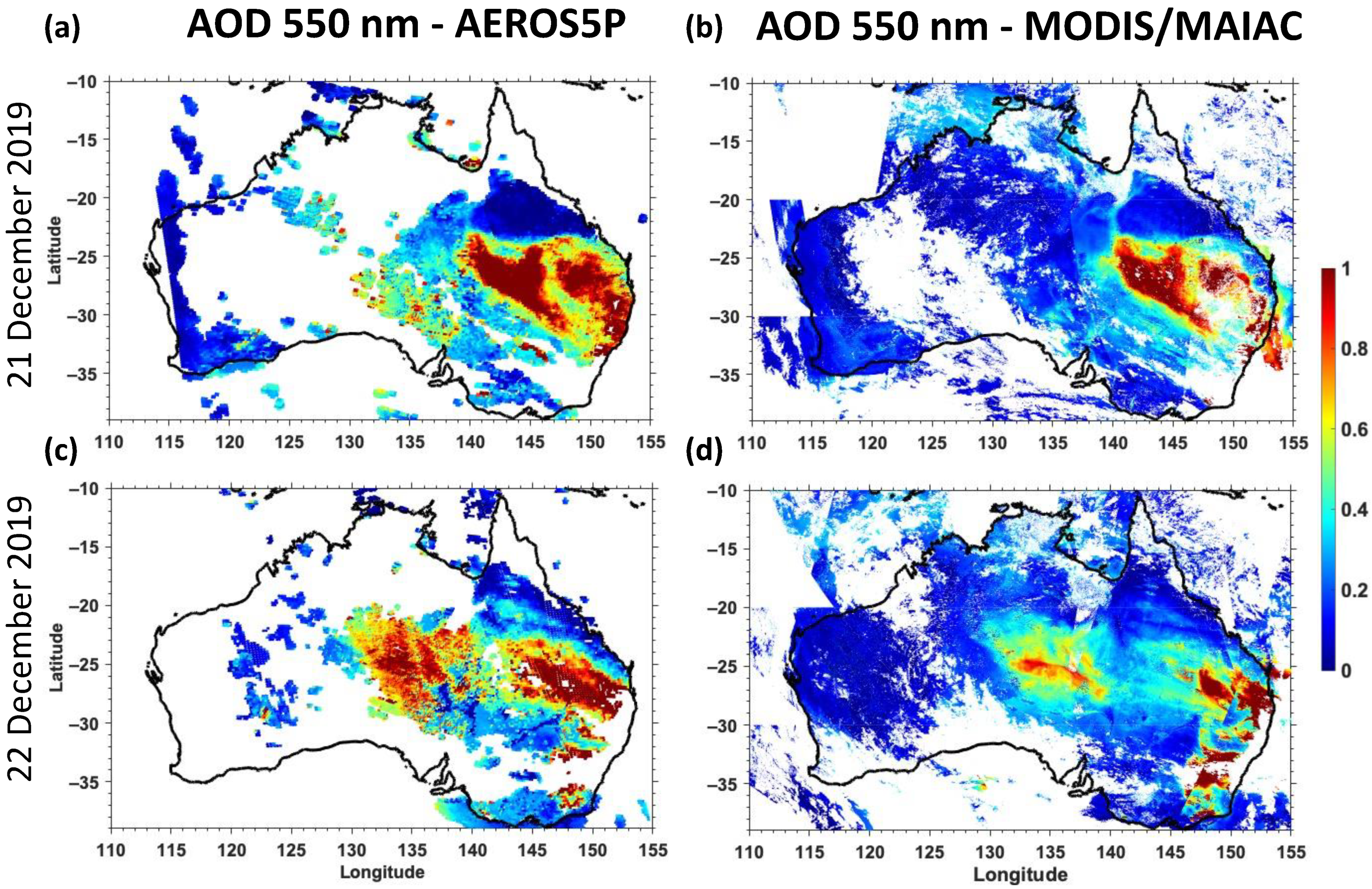
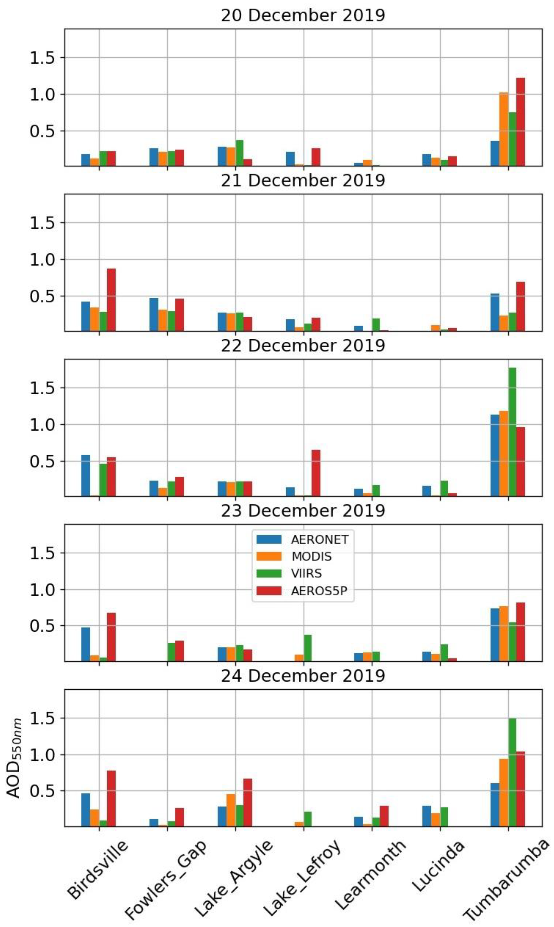
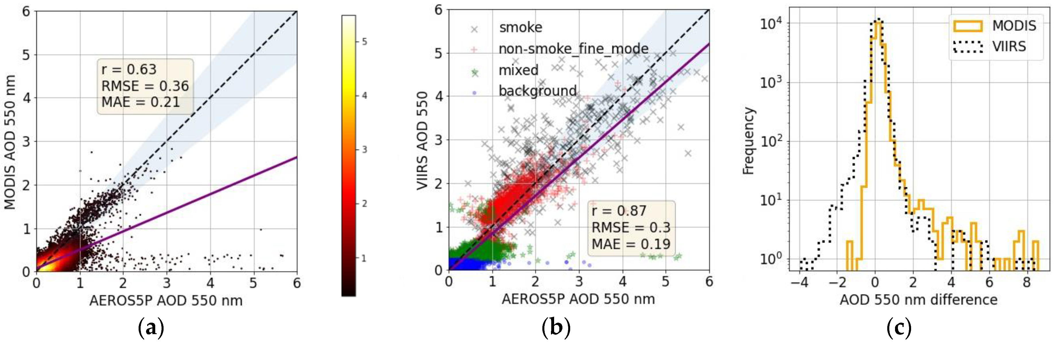
3.1. Aerosol Optical Depth

The horizontal distribution of the AOD observed by AEROS5P was compared to that from MODIS on 20 and 21 December 2019 (Figure 2). The two approaches showed very similar structures of AODs for the two days, both in variability and absolute values. On 20 December, a large and dense BB aerosol plume of an AOD larger than ~1 was depicted over eastern Australia extending from 150°E to 140°E; their shape and AOD values were very similar for both satellites. South and west of the plume some intermediate AODs of up to 0.4 were also seen in both cases. On the following day, two BB aerosol plumes were similarly depicted in two AOD maps. A plume over central Australia of AODs of ~1 and a second one over eastern Australia of AODs above 1 was clearly seen with a similar shape from both satellite data, although moderately larger AODs were seen for AEROS5P. We note a larger horizontal coverage of MODIS/MAIAC data, provided the use of two sensors and a less conservative detection of clouds as compared to AEROS5P. AOD maps from MODIS/Aqua showed overall similar features (not shown for avoiding redundancy) and agreement with AEROS5P, but with a more limited horizontal coverage than MODIS/MAIAC.
Figure 3 presents a comparison of the AOD at 550 nm measured at seven AERONET stations with the three co-located satellite products (AEROS5P, MODIS/Aqua and VIIRS). AOD from AEROS5P was in good agreement with VIIRS and MODIS/Aqua on most of the days of the analyzed intense fire episode on 20–24 December 2021. Daily maps of AOD from AEROS5P compared to these AERONET measurements are shown in the Supplementary Figure S2. The agreements with respect to AERONET ground-based AOD observations are were fairly good and similar for the three satellite products (including AEROS5P). They clearly showed the largest AODs near the fire regions (at Tumbarumba over the southeast of Australia), medium values at central Australia (at Birdsville) downwind from the fires and the lowest ones far from sources (near the eastern coast at Learmonth and Lucinda).
We noticed three cases where the AEROS5P AOD significantly differed from the AERONET measurements. First, on 20 December at the station Tumbarumba, larger AODs were derived by AEROS5P and MODIS (respectively ~1.2 and ~1, around 13:30 local time) than those from AERONET (~0.4, taken around noon). This is clearly linked to the time difference between the measurements, since AERONET measurements at this station showed that AOD rose in the early afternoon of this day up to ~1.2 (according to measurements reported in [63]). The second case occurred on 21 December, when AEROS5P depicted an AOD around 0.9 and the sun photometer from the Birdsville station measured ~0.6. This slight discrepancy likely comes from the horizontal heterogeneity of the smoke plume as nearby AEROS5P retrievals showed AODs around 0.6–0.7 (see Figure S2 on 21 December 2019). The last case of a mismatch between the AOD of AERONET and that of AEROS5P was on 22 December at the station Lake Lefroy. The AEROS5P AOD was then around 0.6 while ~0.1 was measured by the ground-based station. This difference was certainly caused by cloud contamination unfiltered by the VIIRS cloud mask used within AEROS5P. This is consistent with the fact that most nearby pixels were screened out and only isolated pixels near Lake Lefroy showed high AODs (Figure S2). A better cloud filtering mask may improve the retrieval quality in the pixels neighboring cloudy situations.
A more systematic comparison of all co-located retrievals of AOD from AEROS5P, MODIS/Aqua and VIIRS is shown in Figure 4. It covers the period of 20–24 December 2019. A good overall agreement was found between the three datasets, whereas the match was better between AEROS5P and VIIRS. This is shown by the fact that 65% of AEROS5P/VIIRS co-located pixels showed differences smaller than 0.2, a correlation coefficient of 0.87 and RMS differences of 0.3. These values are roughly similar to those found from the comparisons of AOD between MODIS and AEROIASI from the desert dust over the Sahara, with a correlation coefficient of 0.90 and an RMS difference of 0.2 [12,28]. The large value of our RMS difference is likely linked to the large AOD values of the comparison (up to 5 here, where it is at most 1 for [12,28]). With respect to MODIS Aqua, these indicators are moderately smaller, as their correlation coefficient and RMS differences were respectively 0.63 and 0.36, while 58% of the collocated pixels showed AOD differences smaller than 0.2. A mean absolute error around 0.2 is seen between AEROS5P and both other satellite instruments. The range of values of comparison for VIIRS is clearly greater (AOD up to 5) than for the comparison with MODIS, explaining partly the larger correlation in the first case. A comparison by the aerosol type detected by VIIRS shows that larger AOD values were mostly identified as “smoke” as expected (Table 2). Intermediate values with AOD around 0.6 were detected as “non-smoke fine aerosols”. For those two aerosol types (smoke and non-smoke fine aerosols), the match between AEROS5P and VIIRS was much better (correlation coefficient larger than 0.82). Most of the points of AOD below 0.5 correspond to pixels identified by VIIRS as “mixed” and “background” (Table 2). For those cases, the AOD derived from AEROS5P that assumes the presence of only BB aerosols showed as expected larger differences (mainly overestimating) with respect to the retrievals from VIIRS and MODIS.

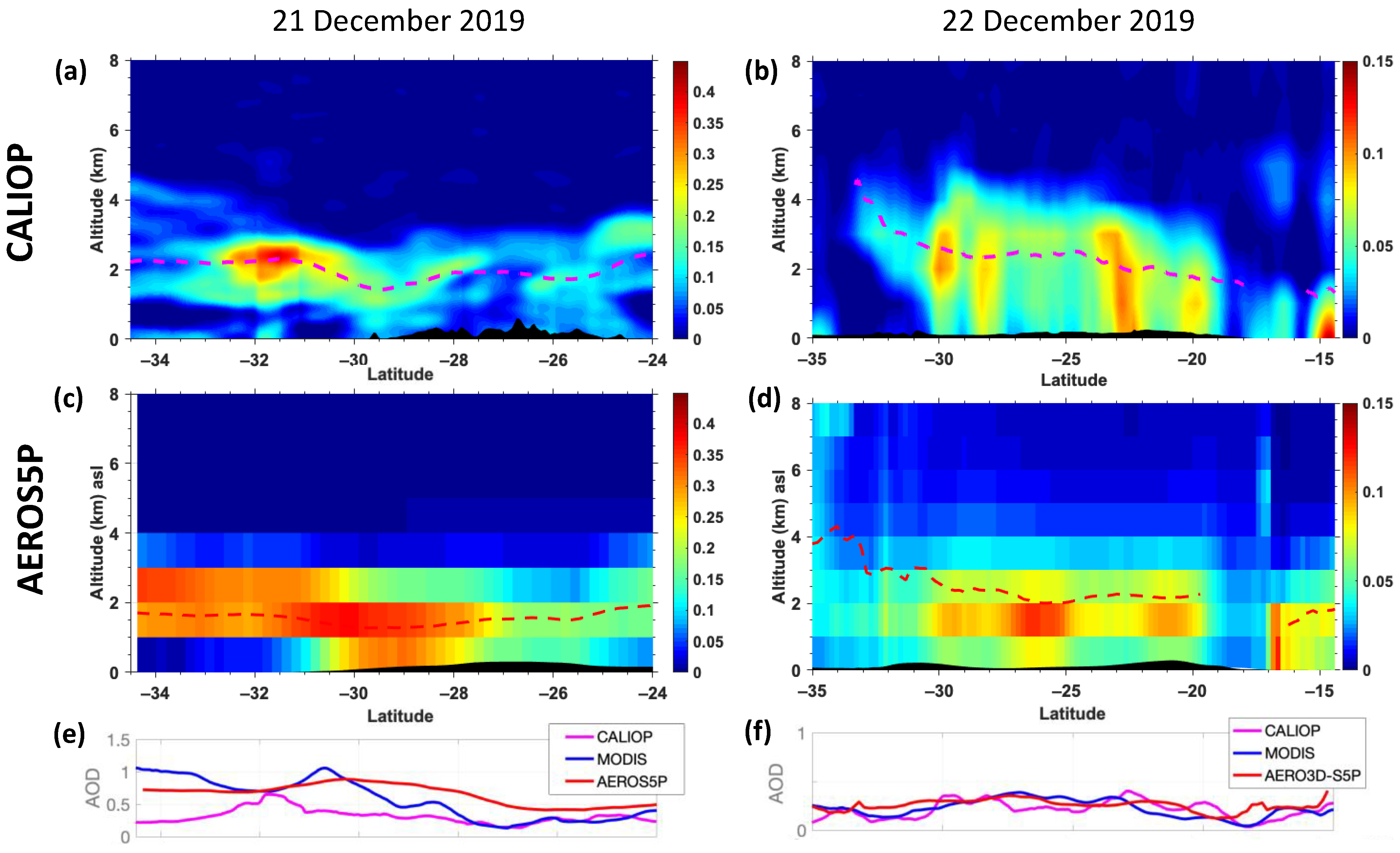
3.2. Aerosol Extinction Profiles

A comparison of two transects of aerosol extinction profiles derived from CALIOP and AEROS5P on 21 and 22 December 2019 is shown in Figure 5. The vertical distribution of aerosols by the two datasets is in fairly good agreement. On 21 December, both retrievals showed a denser aerosol layer extending from 1.0 to about 2.5 km in the southern part, approaching the surface at 28–30°S and progressively increasing in altitude up to 1–3 km around 24°S. The transect of the following day showed in both cases a rather homogenous aerosol layer from the surface up to ~4 km. The aerosol layer top gradually varied from 4 km of altitude at the southern part up to 2 km of altitude near 16°S. Quantitatively, values of aerosol extinction profiles were quite similar between the CALIOP and AEROS5P transects. This particularly stood out on 22 December 2019 (Figure 5b,d), when the vertically integrated AOD for AEROS5P and CALIOP was very similar to that derived from MODIS (Figure 5f). The transect of 21 December 2019 showed moderately larger values of extinction for AEROS5P than those derived from the inversion of CALIOP measurements, while the AOD from AEROS5P was in better agreement with MODIS than that from CALIOP (it underestimated the AOD south of 28°S in Figure 5e). Some other differences may have partly come from the presence of clouds and the difference in overpass times of CALIOP and TROPOMI of about 1.5 h. The mean altitude of the aerosol layers is depicted as dashed lines in the figure. There is a good agreement between the two datasets. Considering all coincidences in the two transects, they show a correlation of 0.83, a mean bias of 180 m and an RMS difference of about 500 m. The uncertainty of the mean aerosol layer height derived from AEROS5P is moderately weaker and in similar order of magnitude to that of the TROPOMI operational product (between 500 and 1000 m according to [71]).

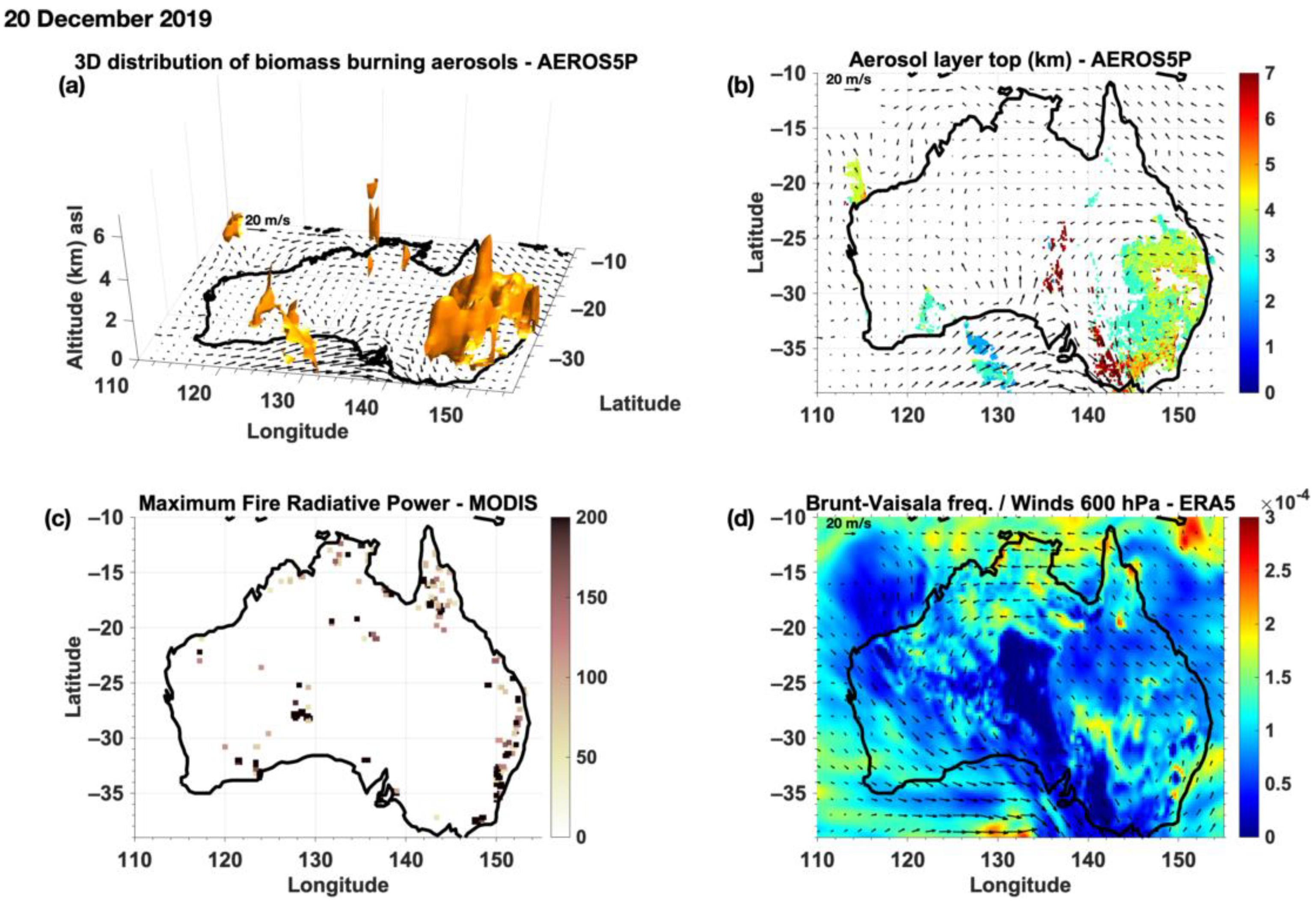
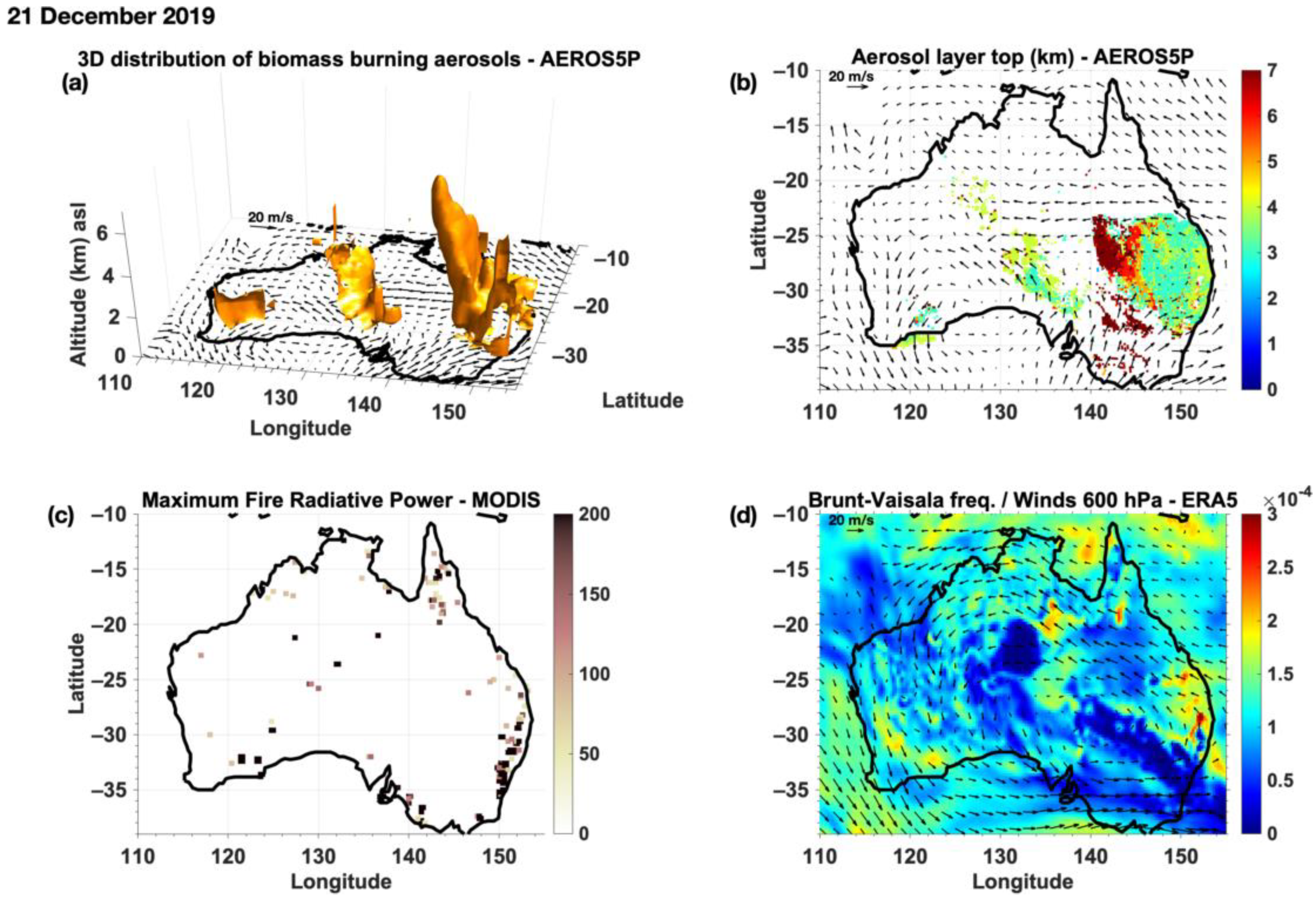
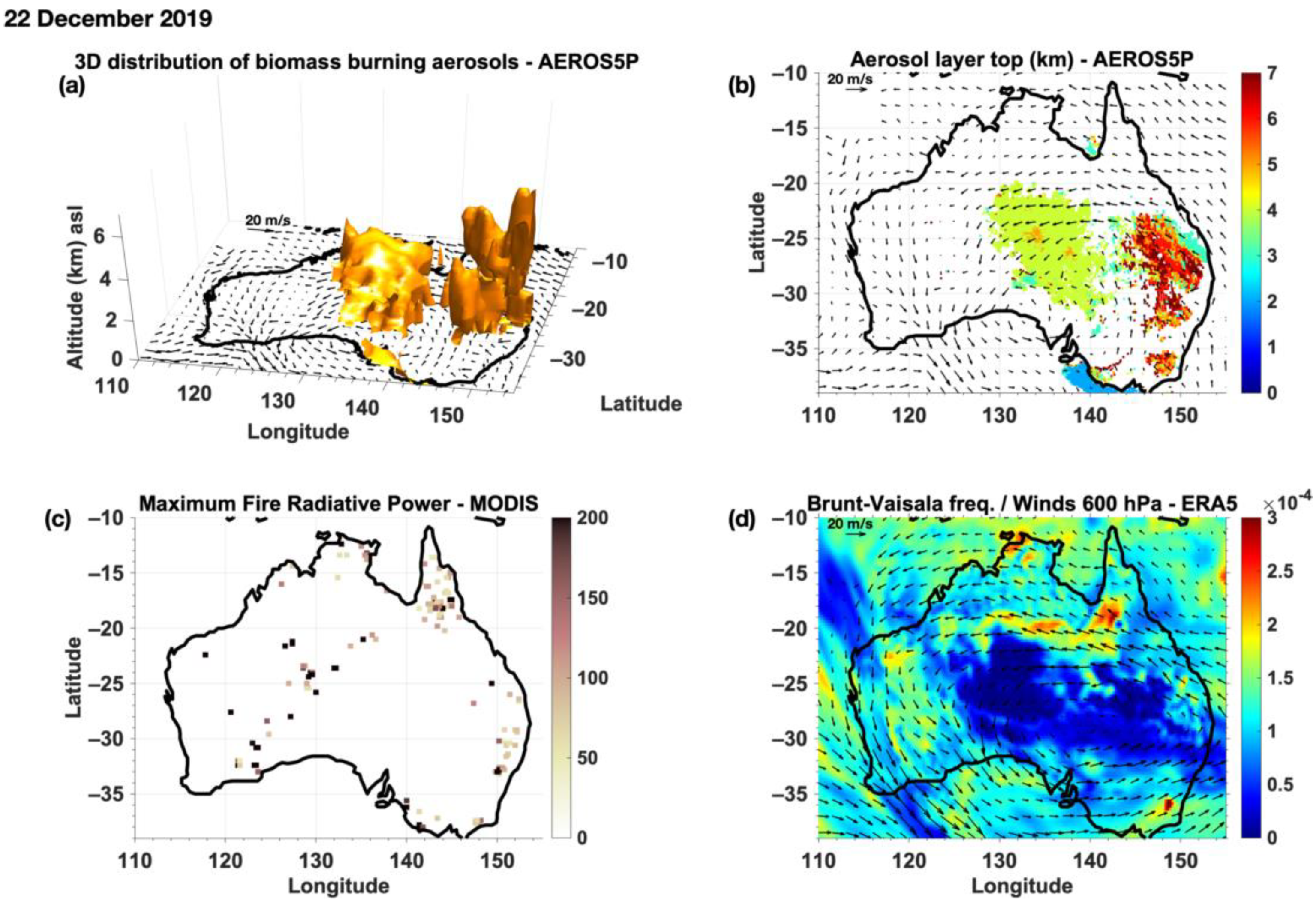
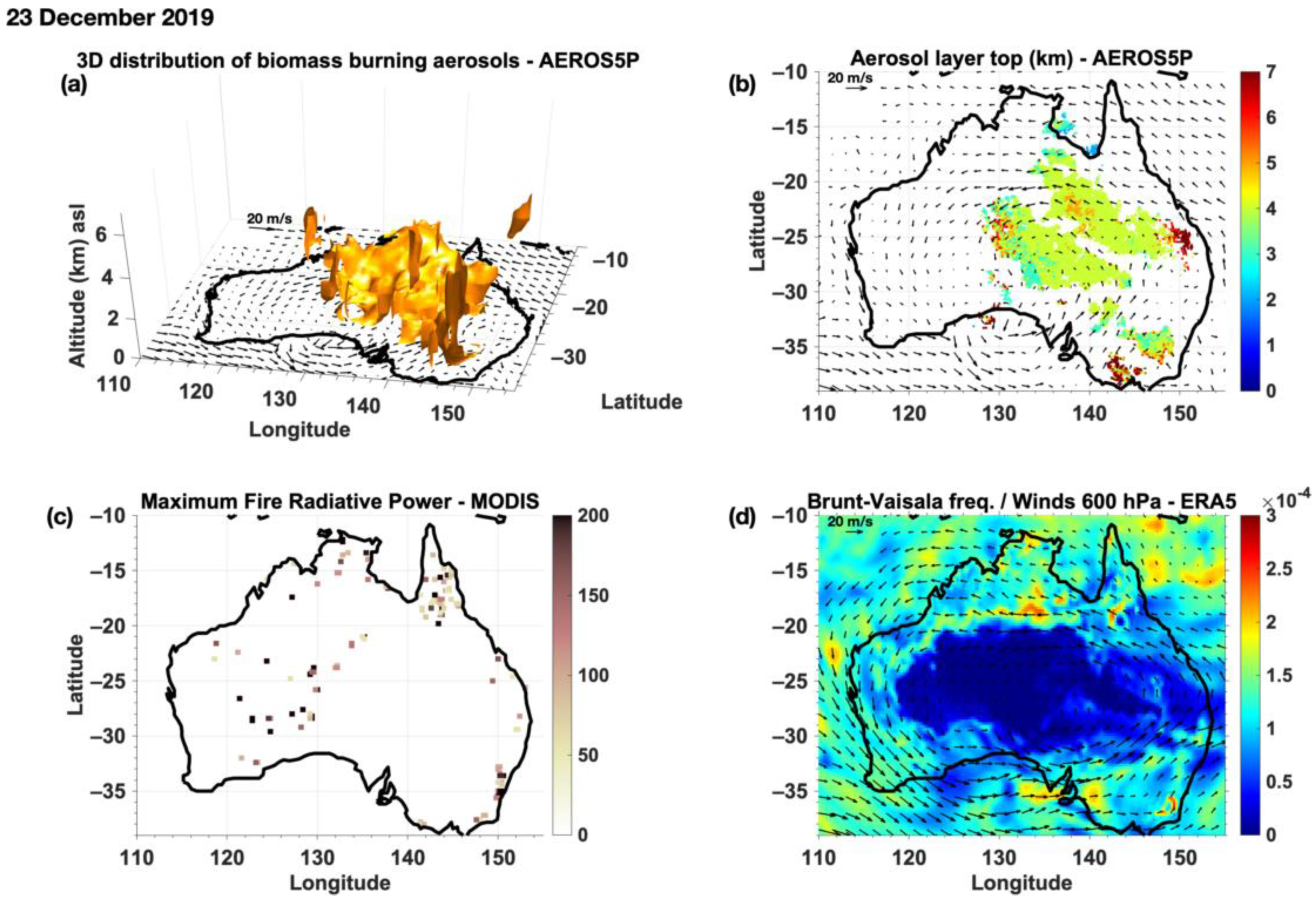
4. Daily Evolution of the 3D Distribution of Biomass Burning Aerosol Plumes

During the period of analysis, exceptionally hot and dry conditions over Australia were responsible for numerous fires in a wide variety of locations. However, the most intense fires leading to the emission of massive amounts of smoke were seen principally located over eastern and southeastern Australia (principally in the New South Wales region [72]. This is seen in the example of fire detections from MODIS on 20 December, where the highest density of fire hotspots was located near the southeastern coast (Figure 6c). As shown in Figure 2 in terms of AOD and also CO retrievals derived from TROPOMI (see Supplementary Figures S2 and S3), the densest smoke plumes were seen over the eastern part of Australia (east of 140°E). The 3D distribution of biomass burning aerosols on 20 December is presented in terms of iso-aerosol extinction surface in Figure 6a. It shows that this large BB aerosols plume located at 25–37°S 140–150°E mainly extended vertically from the surface up to 3–4 km of altitude, with the core plume section reaching 5 km of altitude (seen for some pixels, see the aerosol top heights in Figure 6b). According to estimations of the atmospheric stability in terms of Brunt–Vaisala frequency N2 (calculated at 0.25° degree resolution from ERA5 reanalysis) meteorological conditions at these locations led to a relatively stable atmosphere (values of 1.5 × 10⁻⁴ s−2). Winds at the northern sector of this aerosol plume blew towards the northwestern direction (Figure 6b). The southern and western parts of this aerosol plume reached higher altitudes (5–7 km, seen for some pixels between clouds), co-located with a less stable atmosphere (lower values of N2). Strong winds at 600 hPa (Figure 6d) were expected to transport these aerosols in the southeastern direction over the Pacific.
On 21 December, the density of intense fires at the southeast hotspot (35°S 150°E) enhanced while it diminished elsewhere (Figure 7c). Atmospheric stability was rather low above this region and within a band in the northwestern direction, according to low values of N2 (Figure 7d). As clearly depicted by AEROS5P, the 3D distribution of injections of biomass burning aerosol plumes formed a consistent structure extending from the surface near the fire region and ascending up to 7 km altitude at the northwestern fringe of the plume. The slanted shape of the aerosol plume is consistent with a northwestern direction of the wind at 600 hPa. The eastern part of this large aerosol plume (east of 145°E) extended vertically up to 3–4 km at maximum, which is concomitant with a clearly more vertically stable atmosphere (see higher N2 values in Figure 7d). Other aerosol plumes extending vertically up to 3–4 km (at the south-central part of the continent) were also co-located with rather stable conditions.
On the following day (22 December), the fire activity diminished over the Eastern coast of Australia (Figure 8c). Two aerosol plumes were observed by AEROS5P (Figure 2b,d). The aerosols located at central Australia were likely those emitted the previous day over eastern Australia and then transported northeastward by the winds (see clear and steady wind direction at 850 and 600 hPa in Figure 8b,d). This aerosol plume distributed vertically from the surface up 4–5 km, while being located far from pyro-convective activity of the fire hotspots. The other aerosol plume over eastern Australia was likely freshly emitted by fires. It was injected up to 6 km of altitude (Figure 8a,b), in a region with mostly low atmospheric stability.
On 23 December, wildfire activity was almost absent over the eastern coast of Australia. The two aerosol plumes observed in central Australia by AEROS5P extended vertically up to 4 km of altitude. This limited vertical extent and their geographical location west from the fire regions suggest that they were likely smoke plumes emitted in the previous days. This is consistent with the reduction of new fire emissions on this day. In the absence of a direct link with fire emissions, low atmospheric stability (Figure 9d) did not seem to favor the uplift of these aerosol plumes into higher atmospheric layers. A similar situation is noted on the following day (24 December 2019).
Additionally, we notice that the fire activity detected by MODIS in some regions did not necessarily imply the emission of large amounts of aerosols. This is the case for the example of the Cape York Peninsula located at the northeast of the continent, where fires were detected consistently every day (20–23 December in Figure 6, Figure 7, Figure 8 and Figure 9c) but dense aerosol plumes were not clearly seen as being emitted from this area. This might be linked to the type of vegetation in this area (see Figure S4). Grasslands and savanna are the main vegetation over the Cape York Peninsula, where fire events are more frequent but less intense [73,74]. Over the southeastern coast of the continent, the climate is more temperate and evergreen forests are present. This may explain the emission of large amounts of biomass burning aerosols (e.g., Figure 2) and carbon monoxide (Figure S2) from this area.

5. Conclusions

We presented the new satellite-based AEROS5P approach, which enables the observation of the daily evolution of the 3D distribution of biomass burning aerosols. It was used here to characterize the 3D structure of aerosol plumes emitted by Australian wildfires during late December 2019. This approach derives vertical profiles of aerosol extinction at 550 nm in cloud-free conditions, by analyzing the reflectance spectra in the near infrared and visible measured by TROPOMI at 3.5 × 5.5 km2 resolution. The spectral signature at the oxygen A-band near 760 nm provides information on the altitude of the aerosols, while that in the visible spectrum from 406 to 674 nm provides information about their total column abundance. These two quantities are derived simultaneously.
Aerosol optical depths retrieved by AEROS5P show good agreement with those derived from MODIS and VIIRS, with similar horizontal distribution. These datasets present correlations of up to 0.87 and root-mean-squared differences of 0.3. Transects of vertical profiles of aerosol extinction derived by AEROS5P show similar structures of aerosol plumes to those derived from measurements of the CALIOP spaceborne lidar. Mean altitudes of aerosol layers derived by AEROS5P and CALIOP are also in good agreement. These two datasets show a small mean bias (185 m), root-mean-squared differences of 500 m and a correlation coefficient of 0.83, for the mean plume altitude, for this event.
Moreover, AEROS5P provides an unprecedented daily description of the 3D structure of the vertical injection of smoke plumes. The 3D distribution of these plumes is consistent with fire radiative power hotspots detected by MODIS and atmospheric stability described by a buoyancy frequency diagnostic. For the period of analysis (20–24 December 2019), we remark that aerosol plumes linked with intense fire activities and relatively low atmospheric stability were injected into the atmosphere up to 6 and 7 km of altitude. On the other hand, aerosol plumes extended vertically up to 3–4 km for relatively higher atmospheric stability even near the emission regions. Aerosol plumes reach these altitudes once they are transported far away from sources.
The present paper presents the first application of the AEROS5P approach for a major outbreak of mainly biomass burning aerosols, assuming their microphysical properties for this event. Preliminary tests suggested reasonable performances of the current version of the method for wildfire events in other regions (not shown), for situations without mixing with other aerosol types. As typically done for other satellite aerosol products, we expect better performances using sets of aerosol properties (mainly size and refractive index) adapted for different regions. Future work will be dedicated to consolidating and extending the approach to more diverse situations, such as other periods when BB aerosols from the Australian fires reached the stratosphere or other large fire events in other regions (e.g., Central and South Africa, California, Siberia, etc.). Additional tests on the advantages of jointly adjusting aerosol properties such as size will be considered. Moreover, these studies will include sensitivity analyses on the impact of assumptions and uncertainties of the inputs of the method. More accurate cloud screening is also expected to improve the performance of the method. In addition, future versions of the AEROS5P will also aim at characterizing other types of aerosols such as those from anthropogenic pollution.

Supplementary Materials

The following supporting information can be downloaded at: https://www.mdpi.com/article/10.3390/rs14112582/s1, Figure S1: VIIRS AOD 550 nm per aerosol type from 20 to 24 December 2019, Figure S2: AEROS5P AOD 550 nm from 20 to 24 December 2019. Circles represent the AOD measured by ground-based sun photometer of AERONET stations, Figure S3: TROPOMI Carbon monoxide total column in mol m−2 from 20 to 24 December 2019, Figure S4: MCD12C1 land cover type map for Australia, from ref. [75].

Author Contributions

Investigation, software writing, data curation, formal analysis, writing original draft, performing and analyzing the retrievals, F.L.; Conceptualization, project administration, investigation, methodology, supervision, software writing, analysis, writing—review and editing, funding acquisition, J.C.; Project administration, partial funding acquisition, C.D.; software writing, methodology, M.E.; Project administration, writing—review, G.D.; providing datasets for analysis, G.S.; writing—review, analysis P.S.; writing-review, providing surface albedo principal components, X.L. and P.Z.; writing—review, analysis, fire power data providing, S.T.; Oxygen A-band cross section calculation, D.T.; providing swath dependent soft correction for TROPOMI and writing—review, R.L. and D.L. All authors have read and agreed to the published version of the manuscript.

Funding

This work is funded by the Region Ile-de-France in the framework of the Domaine d’Intérêt Majeur Réseau de recherche Qualité de l’air en Ile-de-France (DIM QI2) through the programme Paris Region PhD (PRPHD), ARIA Technologies, the Programme National de Télédétection Spatiale (PNTS, http://programmes.insu.cnrs.fr/pnts (accessed on 20 April 2022); grant no. PNTS-2016–02, project “AEROMETOP”), and the Centre National des Etudes Spatiales (CNES) through the SURVEYPOLLUTION project from TOSCA (Terre Ocean Surface Continental et Atmosphère), and supported by the Centre National de Recherche Scientifique—Institute National de Sciences de l’Univers (CNRS-INSU) and the Université Paris Est Créteil (UPEC).

Data Availability Statement

The data used in this study was from the following platforms: MODIS AOD data (1 September 2021), MODIS Fire Power (4 October 2021), VIIRS (19 September 2021) data from EarthData portal from NASA (https://search.earthdata.nasa.gov/); CALIOP measurements (13 September 2021) from the AERIS/ICARE datacentre (https://www.aeris-data.fr/ and http://www.icare.univ-lille1.fr/); TROPOMI L1B data (13 July 2020) from the Sentinel 5P hub (https://s5phub.copernicus.eu); TROPOMI Instrument Spectral Response Function (20 May 2020) from: http://www.tropomi.eu; AERONET AOD measurements (16 March 2021) from the AERONET portal (https://aeronet.gsfc.nasa.gov); TROPOMI surface DLER database from Sentinel 5p+ Innovation project (https://www.grasp-sas.com/projects/aod-brdf_sentinel-5p-innovation/); ERA5 meteorological reanalyses (21 September 2021) from the ESPRI IPSL mesocentre (https://mesocentre.ipsl.fr/). The AEROS5P data generated within this work are publicly available on the following repository link: https://trng-b2share.eudat.eu/records/c5ce76e0247547a3b1d276738b9b17de (accessed on 20 May 2022) of the collaborative data infrastructure EUDAT/B2SHARE (https://b2share.eudat.eu).

Acknowledgments

This work is part of the Make Our Planet Great Again (MAPGA) initiative through the project Make Air Quality Great Again (MAQGA) lead by R. Subramanian within the EFLUVE OSU (Observatoire de Sciences de l’Univers) and it is supported by Region Ile-de-France/DIM QI2, PNTS (AEROMETOP project), CNES (SURVEYPOLLUTION/TOSCA project), ARIA Technologies and the ANR ASTuS. We acknowledge the free use of the TROPOMI surface DLER database provided through the Sentinel-5p+ Innovation project of the European Space Agency (ESA). The TROPOMI surface DLER database was created by the Royal Netherlands Meteorological Institute (KNMI) and GRASP SAS (https://www.grasp-sas.com). We are grateful for the free use of the TROPOMI L1b database. We thank Maarten Sneep and Veefkind Pepijn from KNMI for providing help for TROPOMI slit function usage. We acknowledge the free use of MODIS and VIIRS data from NASA’s Earth Observing System Data and Information System (EOSDIS) via Worldview application. We thank ESPRI IPSL mesocentre and the European Centre for Medium Weather Forecast (ECMWF) for providing ERA5 meteorological reanalysis and AERIS/ICARE for the CALIOP lidar data. We acknowledge the free use of data from AErosol RObotic NETwork (AERONET) platform and the PIs of the AERONET sites that have provided their measurements. The authors thank the scientists and researchers who developed and maintain the products of TROPOMI (L1b, CO, ALH); AOD products of MODIS, and VIIRS; cloud-screening from VIIRS; the MODIS Active Fire product; and the CALIOP L1b data, and AOD product from the AERONET stations used in this study. We warmly thank Ha Tran from the Laboratoire de Météorologie Dynamique (LMD), France, for providing the code for calculating Oxygen absorption cross sections in the A-band used in this work.

Conflicts of Interest

The authors declare no conflict of interest.

References

  1. Yu, P.; Davis, S.M.; Toon, O.B.; Portmann, R.W.; Bardeen, C.G.; Barnes, J.E.; Telg, H.; Maloney, C.; Rosenlof, K.H. Persistent Stratospheric Warming Due to 2019–2020 Australian Wildfire Smoke. Geophys. Res. Lett. 2021, 48. [Google Scholar] [CrossRef]
  2. Khaykin, S.; Legras, B.; Bucci, S.; Sellitto, P.; Isaksen, L.; Tencé, F.; Bekki, S.; Bourassa, A.; Rieger, L.; Zawada, D.; et al. The 2019/20 Australian Wildfires Generated a Persistent Smoke-Charged Vortex Rising up to 35 Km Altitude. Commun. Earth Environ. 2020, 1, 22. [Google Scholar] [CrossRef]
  3. Sellitto, P.; Belhadji, R.; Kloss, C.; Legras, B. Radiative Impacts of the Australian Bushfires 2019–2020—Part 1: Large-Scale Radiative Forcing. EGUsphere 2022, 1–20. [Google Scholar] [CrossRef]
  4. Chen, L.; Li, Q.; Wu, D.; Sun, H.; Wei, Y.; Ding, X.; Chen, H.; Cheng, T.; Chen, J. Size distribution and chemical composition of primary particles emitted during open biomass burning processes: Impacts on cloud condensation nuclei activation. Sci. Total Environ. 2019, 674, 179–188. [Google Scholar] [CrossRef]
  5. Li, Y. Cloud Condensation Nuclei Activity and Hygroscopicity of Fresh and Aged Biomass Burning Particles. Pure Appl. Geophys. 2018, 176, 345–356. [Google Scholar] [CrossRef] [Green Version]
  6. Kennedy, I.M. The health effects of combustion-generated aerosols. Proc. Combust. Inst. 2007, 31, 2757–2770. [Google Scholar] [CrossRef]
  7. Freitas, S.R.; Longo, K.M.; Chatfield, R.; Latham, D.; Dias, M.A.F.S.; Andreae, M.O.; Prins, E.; Santos, J.C.; Gielow, R.; Carvalho, J.A., Jr. Including the sub-grid scale plume rise of vegetation fires in low resolution atmospheric transport models. Atmos. Chem. Phys. 2007, 7, 3385–3398. [Google Scholar] [CrossRef] [Green Version]
  8. Turquety, S.; Menut, L.; Siour, G.; Mailler, S.; Hadji-Lazaro, J.; George, M.; Clerbaux, C.; Hurtmans, D.; Coheur, P.-F. APIFLAME v2.0 biomass burning emissions model: Impact of refined input parameters on atmospheric concentration in Portugal in summer 2016. Geosci. Model Dev. 2020, 13, 2981–3009. [Google Scholar] [CrossRef]
  9. Kahn, R.A.; Chen, Y.; Nelson, D.L.; Leung, F.-Y.; Li, Q.; Diner, D.J.; Logan, J.A. Wildfire smoke injection heights: Two perspectives from space. Geophys. Res. Lett. 2008, 35. [Google Scholar] [CrossRef] [Green Version]
  10. Sofiev, M.; Ermakova, T.; Vankevich, R. Evaluation of the smoke-injection height from wild-land fires using remote-sensing data. Atmos. Chem. Phys. 2012, 12, 1995–2006. [Google Scholar] [CrossRef] [Green Version]
  11. Sanders, A.F.J.; de Haan, J.F.; Sneep, M.; Apituley, A.; Stammes, P.; Vieitez, M.O.; Tilstra, L.G.; Tuinder, O.N.E.; Koning, C.E.; Veefkind, J.P. Evaluation of the operational Aerosol Layer Height retrieval algorithm for Sentinel-5 Precursor: Application to O2 A band observations from GOME-2A. Atmos. Meas. Tech. 2015, 8, 4947–4977. [Google Scholar] [CrossRef] [Green Version]
  12. Cuesta, J.; Eremenko, M.; Flamant, C.; Dufour, G.; Laurent, B.; Bergametti, G.; Höpfner, M.; Orphal, J.; Zhou, D. Three-dimensional distribution of a major desert dust outbreak over East Asia in March 2008 derived from IASI satellite observations. J. Geophys. Res. Atmos. 2015, 120, 7099–7127. [Google Scholar] [CrossRef] [Green Version]
  13. Hess, M.; Koepke, P.; Schult, I. Optical Properties of Aerosols and Clouds: The Software Package OPAC. Bull. Am. Meteorol. Soc. 1998, 79, 831–844. [Google Scholar] [CrossRef]
  14. Callies, J.; Corpaccioli, E.; Eisinger, M.; Lefebvre, A.; Munro, R.; Perez-Albinana, A.; Ricciarelli, B.; Calamai, L.; Gironi, G.; Veratti, R.; et al. GOME-2 ozone instrument onboard the European METOP satellites. SPIE Polariz. Sci. Remote Sens. 2004, 5158, 60–70. [Google Scholar] [CrossRef]
  15. Veefkind, J.P.; Aben, I.; McMullan, K.; Förster, H.; de Vries, J.; Otter, G.; Claas, J.; Eskes, H.J.; de Haan, J.F.; Kleipool, Q.; et al. TROPOMI on the ESA Sentinel-5 Precursor: A GMES mission for global observations of the atmospheric composition for climate, air quality and ozone layer applications. Remote Sens. Environ. 2012, 120, 70–83. [Google Scholar] [CrossRef]
  16. Bond, T.C.; Doherty, S.J.; Fahey, D.W.; Forster, P.M.; Berntsen, T.; DeAngelo, B.J.; Flanner, M.G.; Ghan, S.; Kärcher, B.; Koch, D.; et al. Bounding the role of black carbon in the climate system: A scientific assessment. J. Geophys. Res. Atmos. 2013, 118, 5380–5552. [Google Scholar] [CrossRef]
  17. Singh, S.; Fiddler, M.N.; Bililign, S. Measurement of size-dependent single scattering albedo of fresh biomass burning aerosols using the extinction-minus-scattering technique with a combination of cavity ring-down spectroscopy and nephelometry. Atmos. Chem. Phys. 2016, 16, 13491–13507. [Google Scholar] [CrossRef] [Green Version]
  18. Konovalov, I.B.; Golovushkin, N.A.; Beekmann, M.; Andreae, M.O. Insights into the aging of biomass burning aerosol from satellite observations and 3D atmospheric modeling: Evolution of the aerosol optical properties in Siberian wildfire plumes. Atmos. Chem. Phys. 2021, 21, 357–392. [Google Scholar] [CrossRef]
  19. Hosseini, S.; Li, Q.; Cocker, D.; Weise, D.; Miller, A.; Shrivastava, M.; Miller, J.W.; Mahalingam, S.; Princevac, M.; Jung, H. Particle size distributions from laboratory-scale biomass fires using fast response instruments. Atmos. Chem. Phys. 2010, 10, 8065–8076. [Google Scholar] [CrossRef] [Green Version]
  20. Sandvik, O.S.; Friberg, J.; Martinsson, B.G.; Van Velthoven, P.F.J.; Hermann, M.; Zahn, A. Intercomparison of in-situ aircraft and satellite aerosol measurements in the stratosphere. Sci. Rep. 2019, 9, 15576. [Google Scholar] [CrossRef] [Green Version]
  21. Winker, D.M.; Tackett, J.L.; Getzewich, B.J.; Liu, Z.; Vaughan, M.A.; Rogers, R.R. The global 3-D distribution of tropospheric aerosols as characterized by CALIOP. Atmos. Chem. Phys. 2013, 13, 3345–3361. [Google Scholar] [CrossRef] [Green Version]
  22. Chen, X.; Wang, J.; Xu, X.; Zhou, M.; Zhang, H.; Garcia, L.C.; Colarco, P.R.; Janz, S.J.; Yorks, J.; McGill, M.; et al. First retrieval of absorbing aerosol height over dark target using TROPOMI oxygen B band: Algorithm development and application for surface particulate matter estimates. Remote Sens. Environ. 2021, 265, 112674. [Google Scholar] [CrossRef]
  23. Rao, L.; Xu, J.; Efremenko, D.S.; Loyola, D.G.; Doicu, A. Hyperspectral Satellite Remote Sensing of Aerosol Parameters: Sensitivity Analysis and Application to TROPOMI/S5P. Front. Environ. Sci. 2022, 9. [Google Scholar] [CrossRef]
  24. Diner, D.; Beckert, J.; Reilly, T.; Bruegge, C.; Conel, J.; Kahn, R.; Martonchik, J.; Ackerman, T.; Davies, R.; Gerstl, S.; et al. Multi-angle Imaging SpectroRadiometer (MISR) instrument description and experiment overview. IEEE Trans. Geosci. Remote Sens. 1998, 36, 1072–1087. [Google Scholar] [CrossRef]
  25. Limbacher, J.A.; Kahn, R.A. Updated MISR dark water research aerosol retrieval algorithm—Part 1: Coupled 1.1 km ocean surface chlorophyll a retrievals with empirical calibration corrections. Atmos. Meas. Tech. 2017, 10, 1539–1555. [Google Scholar] [CrossRef] [Green Version]
  26. Garay, M.J.; Witek, M.L.; Kahn, R.A.; Seidel, F.C.; Limbacher, J.A.; Bull, M.A.; Diner, D.J.; Hansen, E.G.; Kalashnikova, O.V.; Lee, H.; et al. Introducing the 4.4 Km Spatial Resolution MISR Aerosol Product. Atmos. Meas. Tech. Discuss. 2019, 20, 1–58. [Google Scholar] [CrossRef]
  27. Vandenbussche, S.; Kochenova, S.; Vandaele, A.C.; Kumps, N.; De Mazière, M. Retrieval of Desert Dust Aerosol Vertical Profiles from IASI Measurements in the TIR Atmospheric Window. Atmos. Meas. Tech. 2013, 6, 2577–2591. [Google Scholar] [CrossRef] [Green Version]
  28. Cuesta, J.; Flamant, C.; Eremenko, M.; Dufour, G.; Laurent, B.; Bergametti, G.; Aires, F.; Ryder, C. Three-Dimensional Distribution of a Major Saharan Dust Outbreak in June 2011 Derived from IASI Satellite Observations. In Proceedings of the 4th IASI International Conference, Antibes Juan-les-Pins, France, 11–15 April 2016. [Google Scholar]
  29. Cuesta, J.; Flamant, C.; Gaetani, M.; Knippertz, P.; Fink, A.H.; Chazette, P.; Eremenko, M.; Dufour, G.; Di Biagio, C.; Formenti, P. Three-dimensional pathways of dust over the Sahara during summer 2011 as revealed by new Infrared Atmospheric Sounding Interferometer observations. Q. J. R. Meteorol. Soc. 2020, 146. [Google Scholar] [CrossRef]
  30. Clarisse, L.; Coheur, P.-F.; Prata, F.; Hadji-Lazaro, J.; Hurtmans, D.; Clerbaux, C. A unified approach to infrared aerosol remote sensing and type specification. Atmos. Chem. Phys. 2013, 13, 2195–2221. [Google Scholar] [CrossRef] [Green Version]
  31. Bernath, P.; Boone, C.; Crouse, J. Wildfire smoke destroys stratospheric ozone. Science 2022, 375, 1292–1295. [Google Scholar] [CrossRef]
  32. Guermazi, H.; Sellitto, P.; Cuesta, J.; Eremenko, M.; Lachatre, M.; Mailler, S.; Carboni, E.; Salerno, G.; Caltabiano, T.; Menut, L.; et al. Quantitative Retrieval of Volcanic Sulphate Aerosols from IASI Observations. Remote Sens. 2021, 13, 1808. [Google Scholar] [CrossRef]
  33. Boer, M.M.; Resco De Dios, V.; Bradstock, R.A. Unprecedented burn area of Australian mega forest fires. Nat. Clim. Chang. 2020, 10, 171–172. [Google Scholar] [CrossRef]
  34. Filkov, A.I.; Ngo, T.; Matthews, S.; Telfer, S.; Penman, T.D. Impact of Australia’s Catastrophic 2019/20 Bushfire Season on Communities and Environment. Retrospective Analysis and Current Trends. J. Saf. Sci. Resil. 2020, 1, 44–56. [Google Scholar] [CrossRef]
  35. Steck, T. Methods for determining regularization for atmospheric retrieval problems. Appl. Opt. 2002, 41, 1788–1797. [Google Scholar] [CrossRef]
  36. Liu, X.; Bhartia, P.K.; Chance, K.; Spurr, R.J.D.; Kurosu, T.P. Ozone profile retrievals from the Ozone Monitoring Instrument. Atmos. Chem. Phys. 2010, 10, 2521–2537. [Google Scholar] [CrossRef] [Green Version]
  37. Cuesta, J.; Eremenko, M.; Liu, X.; Dufour, G.; Cai, Z.; Höpfner, M.; von Clarmann, T.; Sellitto, P.; Foret, G.; Gaubert, B.; et al. Satellite observation of lowermost tropospheric ozone by multispectral synergism of IASI thermal infrared and GOME-2 ultraviolet measurements over Europe. Atmos. Chem. Phys. 2013, 13, 9675–9693. [Google Scholar] [CrossRef] [Green Version]
  38. Rodgers, C.D. Inverse Methods For Atmospheric Sounding: Theory and Practice; World Scientific: Singapore, 2000. [Google Scholar]
  39. Wang, P.; Tuinder, O.N.E.; Tilstra, L.G.; de Graaf, M.; Stammes, P. Interpretation of FRESCO cloud retrievals in case of absorbing aerosol events. Atmos. Chem. Phys. 2012, 12, 9057–9077. [Google Scholar] [CrossRef] [Green Version]
  40. Ludewig, A.; Kleipool, Q.; Bartstra, R.; Landzaat, R.; Leloux, J.; Loots, E.; Meijering, P.; van der Plas, E.; Rozemeijer, N.; Vonk, F.; et al. In-flight calibration results of the TROPOMI payload on board the Sentinel-5 Precursor satellite. Atmos. Meas. Tech. 2020, 13, 3561–3580. [Google Scholar] [CrossRef]
  41. Tropomi Monitoring Portal. Available online: http://mps.tropomi.eu/dashboard (accessed on 31 March 2022).
  42. Torres, O.; Tanskanen, A.; Veihelmann, B.; Ahn, C.; Braak, R.; Bhartia, P.; Veefkind, P.; Levelt, P.P. Aerosols and surface UV products from Ozone Monitoring Instrument observations: An overview. J. Geophys. Res. Earth Surf. 2007, 112. [Google Scholar] [CrossRef] [Green Version]
  43. Available online: https://s5phub.copernicus.eu/ (accessed on 6 October 2021).
  44. Platnick, S.; Meyer, K.; Wind, G.; Holz, R.E.; Amarasinghe, N. The NASA MODIS-VIIRS Continuity Cloud Optical Properties Products. Remote Sens. 2021, 13, 2. [Google Scholar] [CrossRef]
  45. Earthdata Search. Available online: https://search.earthdata.nasa.gov/ (accessed on 31 March 2022).
  46. Lutz, R.; Loyola, D.; García, S.G.; Romahn, F. OCRA radiometric cloud fractions for GOME-2 on MetOp-A/B. Atmos. Meas. Tech. 2016, 9, 2357–2379. [Google Scholar] [CrossRef] [Green Version]
  47. Loyola, D.G.; García, S.G.; Lutz, R.; Argyrouli, A.; Romahn, F.; Spurr, R.J.D.; Pedergnana, M.; Doicu, A.; García, V.M.; Schüssler, O. The operational cloud retrieval algorithms from TROPOMI on board Sentinel-5 Precursor. Atmos. Meas. Tech. 2018, 11, 409–427. [Google Scholar] [CrossRef] [Green Version]
  48. Hersbach, H.; Bell, B.; Berrisford, P.; Hirahara, S.; Horányi, A.; Muñoz-Sabater, J.; Nicolas, J.; Peubey, C.; Radu, R.; Schepers, D.; et al. The ERA5 global reanalysis. Q. J. R. Meteorol. Soc. 2020, 146, 1999–2049. [Google Scholar] [CrossRef]
  49. Rothman, L.S.; Gordon, I.E.; Babikov, Y.; Barbe, A.; Benner, D.C.; Bernath, P.F.; Birk, M.; Bizzocchi, L.; Boudon, V.; Brown, L.R.; et al. The HITRAN2012 molecular spectroscopic database. J. Quant. Spectrosc. Radiat. Transf. 2013, 130, 4–50. [Google Scholar] [CrossRef] [Green Version]
  50. Chance, K.; Kurucz, R. An improved high-resolution solar reference spectrum for earth’s atmosphere measurements in the ultraviolet, visible, and near infrared. J. Quant. Spectrosc. Radiat. Transf. 2010, 111, 1289–1295. [Google Scholar] [CrossRef]
  51. Sentinel-5p+ Innovation. Available online: https://www.grasp-sas.com/projects/aod-brdf_sentinel-5p-innovation/ (accessed on 31 March 2022).
  52. Sarpong, E.; Smith, D.; Pokhrel, R.; Fiddler, M.N.; Bililign, S. Refractive Indices of Biomass Burning Aerosols Obtained from African Biomass Fuels Using RDG Approximation. Atmosphere 2020, 11, 62. [Google Scholar] [CrossRef] [Green Version]
  53. Tran, H.; Boulet, C.; Hartmann, J.-M. Line mixing and collision-induced absorption by oxygen in the A band: Laboratory measurements, model, and tools for atmospheric spectra computations. J. Geophys. Res. Earth Surf. 2006, 111. [Google Scholar] [CrossRef] [Green Version]
  54. ISRF Dataset. Tropomi. Available online: http://www.tropomi.eu/data-products/isrf-dataset (accessed on 31 March 2022).
  55. Spurr, R.J. VLIDORT: A linearized pseudo-spherical vector discrete ordinate radiative transfer code for forward model and retrieval studies in multilayer multiple scattering media. J. Quant. Spectrosc. Radiat. Transf. 2006, 102, 316–342. [Google Scholar] [CrossRef]
  56. Spurr, R.; Christi, M. On the generation of atmospheric property Jacobians from the (V)LIDORT linearized radiative transfer models. J. Quant. Spectrosc. Radiat. Transf. 2014, 142, 109–115. [Google Scholar] [CrossRef]
  57. Peterson, D.A.; Fromm, M.D.; McRae, R.H.D.; Campbell, J.R.; Hyer, E.J.; Taha, G.; Camacho, C.P.; Kablick, G.P.; Schmidt, C.C.; DeLand, M.T. Australia’s Black Summer pyrocumulonimbus super outbreak reveals potential for increasingly extreme stratospheric smoke events. NPJ Clim. Atmos. Sci. 2021, 4, 1–16. [Google Scholar] [CrossRef]
  58. Zoogman, P.; Liu, X.; Chance, K.; Sun, Q.; Schaaf, C.; Mahr, T.; Wagner, T. A climatology of visible surface reflectance spectra. J. Quant. Spectrosc. Radiat. Transf. 2016, 180, 39–46. [Google Scholar] [CrossRef]
  59. Clark, R.N.; Swayze, G.A.; Wise, R.A.; Livo, K.E.; Hoefen, T.M.; Kokaly, R.F.; Sutley, S.J. USGS Digital Spectral Library splib06a; US Geological Survey: Denver, CO, USA, 2007.
  60. Tikhonov, A.N. On the Solution of Ill-Posed Problems and the Method of Regularization. In Doklady Akademii Nauk; Russian Academy of Sciences: Saint Petersburg, Russia, 1963; Volume 151, pp. 501–504. [Google Scholar]
  61. Eremenko, M.; Dufour, G.; Foret, G.; Keim, C.; Orphal, J.; Beekmann, M.; Bergametti, G.; Flaud, J.-M. Tropospheric ozone distributions over Europe during the heat wave in July 2007 observed from infrared nadir spectra recorded by IASI. Geophys. Res. Lett. 2008, 35. [Google Scholar] [CrossRef]
  62. Giles, D.M.; Sinyuk, A.; Sorokin, M.G.; Schafer, J.S.; Smirnov, A.; Slutsker, I.; Eck, T.F.; Holben, B.N.; Lewis, J.R.; Campbell, J.R.; et al. Advancements in the Aerosol Robotic Network (AERONET) Version 3 database – automated near-real-time quality control algorithm with improved cloud screening for Sun photometer aerosol optical depth (AOD) measurements. Atmos. Meas. Tech. 2019, 12, 169–209. [Google Scholar] [CrossRef] [Green Version]
  63. AERONET, Aerosol Robotic Network. Available online: https://aeronet.gsfc.nasa.gov/ (accessed on 10 January 2020).
  64. Bilal, M.; Qiu, Z.; Campbell, J.R.; Spak, S.N.; Shen, X.; Nazeer, M. A New MODIS C6 Dark Target and Deep Blue Merged Aerosol Product on a 3 km Spatial Grid. Remote Sens. 2018, 10, 463. [Google Scholar] [CrossRef] [Green Version]
  65. Fernald, F.G. Analysis of atmospheric lidar observations: Some comments. Appl. Opt. 1984, 23, 652–653. [Google Scholar] [CrossRef]
  66. Fernald, F.G.; Herman, B.M.; Reagan, J.A. Determination of Aerosol Height Distributions by Lidar. J. Appl. Meteorol. 1972, 11, 482–489. [Google Scholar] [CrossRef] [Green Version]
  67. Landgraf, J.; de Brugh, J.A.; Scheepmaker, R.; Borsdorff, T.; Hu, H.; Houweling, S.; Butz, A.; Aben, I.; Hasekamp, O. Carbon monoxide total column retrievals from TROPOMI shortwave infrared measurements. Atmos. Meas. Tech. 2016, 9, 4955–4975. [Google Scholar] [CrossRef] [Green Version]
  68. Borsdorff, T.; de Brugh, J.A.; Hu, H.; Hasekamp, O.; Sussmann, R.; Rettinger, M.; Hase, F.; Gross, J.; Schneider, M.; Garcia, O.; et al. Mapping carbon monoxide pollution from space down to city scales with daily global coverage. Atmos. Meas. Tech. 2018, 11, 5507–5518. [Google Scholar] [CrossRef] [Green Version]
  69. Giglio, L.; Schroeder, W.; Justice, C.O. The collection 6 MODIS active fire detection algorithm and fire products. Remote Sens. Environ. 2016, 178, 31–41. [Google Scholar] [CrossRef] [Green Version]
  70. Stull, R.B. An Introduction to Boundary Layer Meteorology; Springer Science & Business Media: Berlin/Heidelberg, Germany, 1988. [Google Scholar]
  71. Nanda, S.; de Graaf, M.; Veefkind, J.P.; Sneep, M.; ter Linden, M.; Sun, J.; Levelt, P.F. A first comparison of TROPOMI aerosol layer height (ALH) to CALIOP data. Atmos. Meas. Tech. 2020, 13, 3043–3059. [Google Scholar] [CrossRef]
  72. Kloss, C.; Sellitto, P.; von Hobe, M.; Berthet, G.; Smale, D.; Krysztofiak, G.; Xue, C.; Qiu, C.; Jégou, F.; Ouerghemmi, I.; et al. Australian Fires 2019–2020: Tropospheric and Stratospheric Pollution Throughout the Whole Fire Season. Front. Environ. Sci. 2021, 9, 652024. [Google Scholar] [CrossRef]
  73. Beringer, J.; Hutley, L.B.; Abramson, D.; Arndt, S.K.; Briggs, P.; Bristow, M.; Canadell, J.G.; Cernusak, L.A.; Eamus, D.; Edwards, A.C.; et al. Fire in Australian savannas: From leaf to landscape. Glob. Chang. Biol. 2014, 21, 62–81. [Google Scholar] [CrossRef] [PubMed] [Green Version]
  74. Williams, R.J.; Gill, A.M.; Moore, P.H.R. Seasonal Changes in Fire Behaviour in a Tropical Savanna in Northern Australia. Int. J. Wildland Fire 1998, 8, 227–239. [Google Scholar] [CrossRef]
  75. Chaivaranont, W.; Evans, J.P.; Liu, Y.Y.; Sharples, J.J. Estimating grassland curing with remotely sensed data. Nat. Hazards Earth Syst. Sci. 2018, 18, 1535–1554. [Google Scholar] [CrossRef] [Green Version]
Figure 1. Scheme of the AEROS5P algorithm for retrieving the 3D distribution of fine BB aerosols. r: aerosol size distribution modal radius; s: aerosol size distribution standard deviation; hmean: aerosol layer mean height; α550: aerosol extinction profile at 550 nm; htop: aerosol layer top height; AOD550: aerosol optical depth at 550 nm.
Remotesensing 14 02582 g001
Figure 2. Horizontal distribution of AODs at 550 nm from (a,c) AEROS5P and (b,d) MODIS using the MAIAC algorithm on (a,b) 21 and (c,d) 22 December 2019 over Australia. This period was characterized by intense wildfires with large emission of BB aerosols.
Remotesensing 14 02582 g002
Figure 3. Comparison of AOD at 550 nm measured at 7 AERONET stations in Australia by sun photometer with respect to three satellite products: AEROS5P, MODIS/Aqua and VIIRS on 20 to 24 December 2019 (one panel per day from the upper to lower one).
Remotesensing 14 02582 g003
Figure 4. Scatterplot comparison of AOD at 550 nm derived from AEROS5P with respect to co-located retrievals from (a) MODIS/AQUA and (b) VIIRS for the period 20–24 December 2019. Colors in panel (a) represent the number of points for each sector of 0.1 × 0.1 of AOD. For (a,b), purple lines are linear regression lines of the scatter of points, dotted lines are the 1:1 curve and blue shade is the ±20% interval. (c) Frequency histogram of differences of AOD at 550 nm of MODIS/AQUA and VIIRS with respect to AEROS5P. Symbols and colors in panel (b) indicate the aerosol type derived from the VIIRS approach.
Remotesensing 14 02582 g004
Figure 5. Comparison of transects of aerosol extinction profiles (in km−1) derived from (a,b) the CALIOP spaceborne lidar and (c,d) the AEROS5P passive approach on (a,c) 21 December and (b,d) 22 December 2019. Dashed lines indicate the mean altitude of the aerosol layers defined as the ones with half of the AOD above and below. The corresponding AOD at 550 nm from MODIS MAIAC and AEROS5P, and CALIOP at 532 nm is shown in panels (e,f).
Remotesensing 14 02582 g005
Figure 6. (a) Three-dimensional distribution of biomass burning aerosols on 20 December 2019 derived from TROPOMI measurements using the AEROS5P method, depicted as iso-aerosol extinction surface of 0.1 km−1. (b) Aerosol layer top derived from AEROS5P as the aerosol highest layer with aerosol extinction larger than 0.1 km−1. (c) Maximum fire radiative power derived from MODIS sensors onboard Aqua and Terra within each 0.2 × 0.2° grid pixel. (d) Static atmospheric stability depicted by the Brunt–Vaisala frequency derived from ERA5 reanalysis. Winds from ERA5 reanalysis are overlaid on panels (a,b) at 850 hPa and (d) at 600 hPa. For clarity, wind speed scales are shown in the upper left corners and wind vectors are displayed for each 1.5 × 1.5° grid point.
Remotesensing 14 02582 g006
Figure 7. Same as Figure 6 but for 21 December 2019.
Remotesensing 14 02582 g007
Figure 8. Same as Figure 6 but for 22 December 2019.
Remotesensing 14 02582 g008
Figure 9. Same as Figure 6 but for 23 December 2019.
Remotesensing 14 02582 g009
Table 1. AEROS5P inputs and their corresponding sources.
VariableCharacteristics
TROPOMI measurementsReflectance spectra12 microwindows * at 406, 416, 425, 436, 442, 451.5, 463, 477, 483, 494.5, 674.5 and 766.5 nm
Meteorological stateTemperature profileERAI reanalyzes
Pressure profileERAI reanalyzes
Water vapor profileERAI reanalyzes
Atmospheric speciesA unique a priori aerosol concentration profileHomogeneous concentration up to 9 km corresponding to a background AOD of 0.03 at 550 nm
BB aerosol refractive indicesFrom [52]
Oxygen vertical profileA constant mixing ratio of 0.209
Aerosol size distributionA modal radius around 0.1 µm and width of 1.43 taken from
AERONET retrievals at Birdsville on 22 December 2019
Gas absorption cross sectionsOxygen absorption cross sectionsCalculation using HITRAN 2012 [49] spectroscopic parameters, line mixing, H2O broadening and collision-induced absorption
following [53]
H2O absorption cross sectionsFrom HITRAN 2012 [49]
Geophysical stateSolar spectrumHigh spectral measurements from [50]
Surface albedoDLER at 19 wavelengths, 0.125 × 0.125°, version 0.3 from the
TROPOMI s5p+ Innovation project [51]
Instrumental calibrationSoft correctionAdapted from the soft correction for the OCRA cloud retrieval [46,47]
Instrumental spectral responseSlit function provided for each swath position and wavelengths from [54]
* Central wavelengths indicated.
Table 2. Comparison of AOD from AEROS5P and VIIRS for each aerosol type detected by VIIRS. r: Pearson correlation coefficient; RMSE: Root Mean Squared Error; MAE: Mean Absolute Error.
Aerosol TyperRMSEMAENumber of Co-Located Pixels
Smoke0.820.690.49667
Non-smoke fine mode0.860.300.243168
Mixed0.230.350.215868
Background0.240.200.138595
Publisher’s Note: MDPI stays neutral with regard to jurisdictional claims in published maps and institutional affiliations.

