Article

Monitoring 2019 Drought and Assessing Its Effects on Vegetation Using Solar-Induced Chlorophyll Fluorescence and Vegetation Indexes in the Middle and Lower Reaches of Yangtze River, China

1
College of Resources and Environment, Anhui Agricultural University, Hefei 230036, China
2
Anhui Public Meteorological Service Center, Anhui Meteorological Bureau, Hefei 230031, China
3
The Weather Modification Center of Henan Province, Zhengzhou 450003, China
4
Key Laboratory of Meteorological Disaster, Ministry of Education (KLME), Joint International Research Laboratory of Climate and Environment Change (ILCEC), Collaborative Innovation Center on Forecast and Evaluation of Meteorological Disasters (CIC-FEMD), Jiangsu Key Laboratory of Agricultural Meteorology, College of Applied Meteorology, Nanjing University of Information Science & Technology, Nanjing 210044, China
5
Department of Disaster Management, Begum Rokeya University, Rangpur 5400, Bangladesh
*
Author to whom correspondence should be addressed.
These authors contributed equally to this work.
Remote Sens. 2022, 14(11), 2569; https://doi.org/10.3390/rs14112569
Submission received: 30 March 2022 / Revised: 12 May 2022 / Accepted: 23 May 2022 / Published: 27 May 2022

Abstract

:
Monitoring drought precisely and evaluating drought effects quantitatively can establish a scientific foundation for understanding drought. Although solar-induced chlorophyll fluorescence (SIF) can detect the drought stress in advance, the performance of SIF in monitoring drought and assessing drought-induced gross primary productivity (GPP) losses from lush to senescence remains to be further studied. Taking the 2019 drought in the middle and lower reaches of the Yangtze River (MLRYR) as an example, this study aims to monitor and assess this drought by employing a new global, OCO-2-based SIF (GOSIF) and vegetation indexes (VIs). Results showed that the GPP, GOSIF, and VIs all exhibited significant increasing trends during 2000–2020. GOSIF was most consistent with GPP in spatial distribution and was most correlated with GPP in both annual (linear correlation, R2 = 0.87) and monthly (polynomial correlation, R2 = 0.976) time scales by comparing with VIs. During July–December 2019, the precipitation (PPT), soil moisture, and standardized precipitation evapotranspiration index (SPEI) were generally below the averages during 2011–2020 and reached their lowest point in November, while those of air temperature (Tem), land surface temperature (LST), and photosynthetically active radiation (PAR) were the contrary. For drought monitoring, the spatial distributions of standardized anomalies of GOSIF and VIs were consistent during August–October 2019. In November and December, however, considering vegetation has entered the senescence stage, SIF had an obvious early response in vegetation physiological state monitoring compared with VIs, while VIs can better indicate meteorological drought conditions than SIF. For drought assessment, the spatial distribution characteristics of GOSIF and its standardized anomaly were both most consistent with that of GPP, especially the standardized anomaly in November and December. All the above phenomena verified the good spatial consistency between SIF and GPP and the superior ability of SIF in capturing and quantifying drought-induced GPP losses. Results of this study will improve the understanding of the prevention and reduction in agrometeorological disasters and can provide an accurate and timely method for drought monitoring.

Graphical Abstract

1. Introduction

Drought is a complex process involving soil, vegetation, the atmosphere, and other factors. The decrease in precipitation and the increase in air temperature will often cause a rise in surface evapotranspiration and lead to drought occurrence and intensification, which will bring significant uncertainty to drought monitoring [1]. In the context of global climate change, drought, as one of the longest and most destructive extreme climate events, has been a concern by scholars worldwide for a long time. The occurrence of large-scale drought events tends to weaken carbon deposition in terrestrial ecosystems and exacerbate the conflict between food demand and biofuel production [2]. Moreover, the occurrence of extreme drought events, even in areas with well-irrigated facilities, can also have a significant impact on food production and the social economy [3]. It is reported that by the end of the 21st century, the global annual average air temperature is expected to rise by 0.3~4.8 °C, and the probability of drought occurrence will also increase under future climate scenarios, which will pose a significant risk to vegetation growth [4]; therefore, it is crucial to study the spatial–temporal evolution characteristics of drought events and evaluate their impacts quantitatively.
With the rapid development of satellite remote sensing technology, it is now possible to observe drought characteristics at regional and global scales continuously, especially in areas with limited field observation data, which also provides a new way to monitor and assess the impact of large-scale drought events on surface vegetation [5]. The vegetation index obtained from remote sensing data is a quantitative indicator of vegetation greenness, which can indirectly reflect vegetation’s physiological state. Presently, traditional vegetation indexes (VIs, such as normalized differential vegetation index (NDVI) and enhanced vegetation index (EVI)) have been widely used to monitor the vegetation’s physiological state and evaluate the effect of water stress on vegetation productivity. Although traditional VIs can represent the physiological state of vegetation, they can only reflect the vegetation’s pigment content change, which is not directly related to the actual photosynthesis of plants, let alone the evolution of their instantaneous photosynthetic rate [6]; therefore, the response of traditional VIs to the situation of vegetation water loss is slow, cannot reflect the dynamic response process of vegetation to various water stresses immediately and has an evident lag in capturing vegetation drought information, which highly restricts its applicability in early drought monitoring [7,8]. Solar-induced chlorophyll fluorescence (SIF) is a spectral signal (650~800 nm) emitted by the photosynthetic center of chlorophyll molecules in the form of fluorescence under solar illumination conditions, with two peaks in the red band (about 690 nm) and near-infrared band (about 740 nm) [9]. Solar radiation absorbed by vegetation can be used for photosynthesis, heat dissipation, and re-release of fluorescence. Of those, chlorophyll fluorescence is the energy re-stimulated by vegetation photosynthesis after absorbing light, so it can directly reflect the dynamic changes of a plant’s actual photosynthesis [10]. As a direct probe of the plant’s actual photosynthesis, compared with traditional VIs, SIF can achieve rapid response and early warning when plants are subjected to environmental stress (such as water stress, heat stress, etc.) [6,7,8,11]. In recent years, global SIF remote sensing datasets have been successfully retrieved from SCIAMACHY, GOSAT, GOME-2, OCO-2, TROPOMI, and other space-borne sensors, making it possible to study plant photosynthesis on a large scale and providing new data sources for regional vegetation growth and environmental stress monitoring [9,12]. At present, SIF data based on satellite inversion has been adopted to monitor and evaluate large-scale drought events in Russia [13], Texas, the central great plains of the United States [14,15,16], Europe [17], Yunnan province [8], the North China plain [6] of China, Australia [1,18], etc.
As one of the main abiotic stress factors affecting plant growth and production, drought can directly or indirectly inhibit photosynthesis [19]. The inhibition of photosynthesis by drought stress can be divided into stomatal and non-stomatal restrictions. Stomatal restriction mainly refers to the decline of leaf water potential and the stomatal closure in mild drought conditions, which inhibits photosynthesis by limiting the entry of photosynthetic substances (carbon dioxide, CO2) into plants. The non-stomatal restriction generally refers to the damage to the protein metabolic process of the photosynthetic system II reaction center and the changes in chloroplast structure of crops caused by severe drought, which inhibits the activity of Rubisco activase, thus reducing plant photosynthesis [20,21]. Gross primary productivity (GPP) reflects the ability of green plants to produce organic matter through photosynthesis. It measures the photosynthetic rate and is a crucial component of the global carbon cycle. Studies have shown that SIF is directly related to the actual photosynthesis of plants, and the good linear relationship between SIF and GPP provides a direct method for remote sensing estimation of GPP [22]; however, when plants are suffering from environmental stresses (e.g., drought and heatwave), the linear relationship between SIF and GPP will be uncertain, which will lead to a decrease in the accuracy of vegetation GPP monitoring by remote sensing under stress [23]; therefore, further exploration of the effects of drought stress on the SIF-GPP relationship is of paramount significance for assessing the ability of SIF to capture and quantify drought-induced GPP losses.
To the best of the author’s knowledge, few studies have been undertaken to explore the recent 2019 drought impacts on vegetation in the middle and lower reaches of the Yangtze River (MLRYR). Moreover, the performance of SIF in drought monitoring and in assessing drought-induced GPP losses during vegetation growth from lush to senescence still needs to be further investigated. Thus, the specific objectives of this study are (1) to investigate the spatiotemporal variations of GPP, GOSIF, and VIs during 2000–2020; (2) to analyze the spatiotemporal evolution characteristics of the continuous drought in summer and autumn from July to December in 2019; (3) to evaluate the impacts of drought on vegetation physiological and ecological indicators and reveal the performance of SIF in vegetation drought monitoring; (4) to explore the effects of drought on vegetation productivity and clarify the potential of SIF in capturing and quantifying drought-induced GPP losses.

2. Materials and Methods
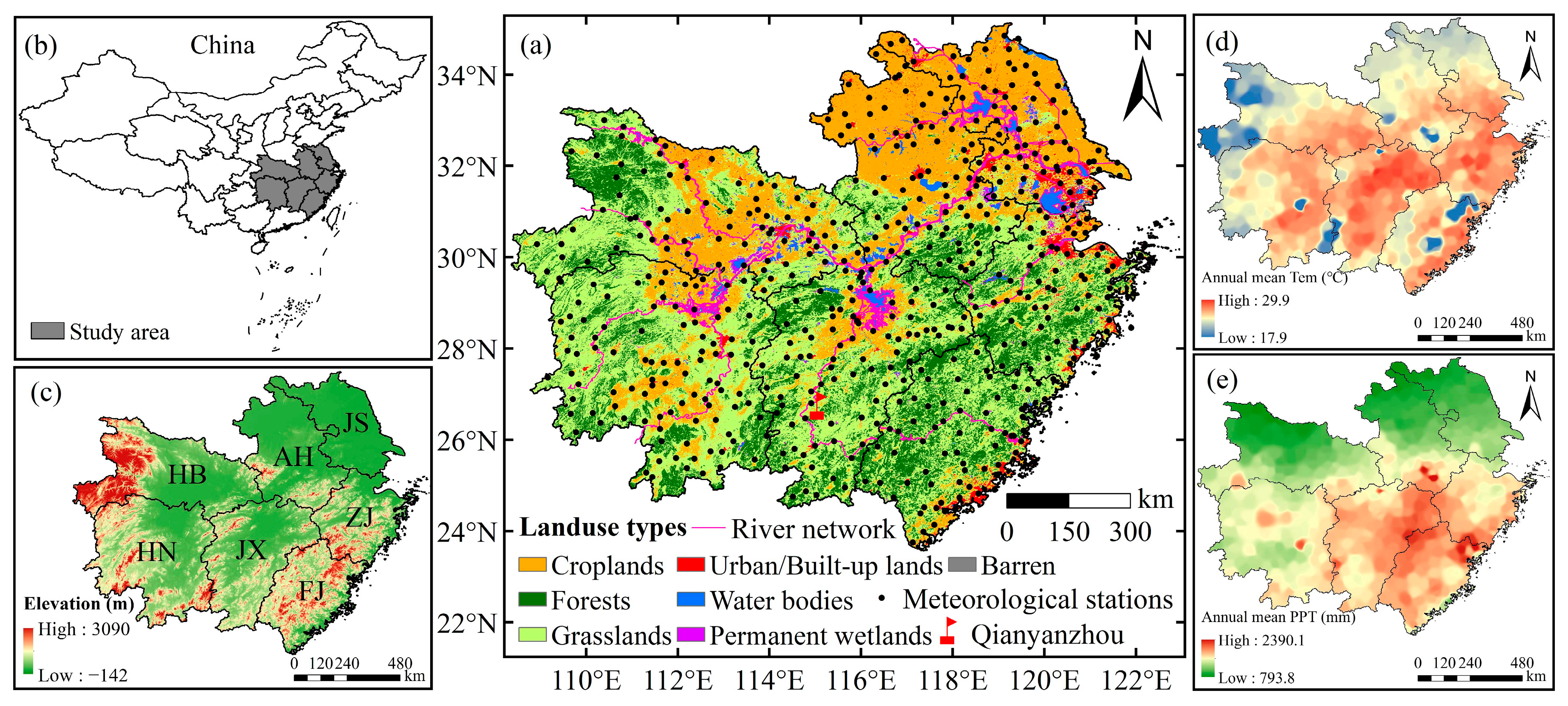
2.1. Study Area

The MLRYR region (23°33′~35°08′N, 108°21′~123°10′E), including Hubei, Hunan, Anhui, Jiangxi, Jiangsu, Zhejiang, and Fujian provinces, has a subtropical monsoon climate with a warm temperature and abundant precipitation, and is a crucial grain, oil, and cotton production base in China [24] (Figure 1b,c). The land-use types in this region are croplands, forests, grasslands, urban/built-up lands, water bodies, permanent wetlands, and barren (Figure 1a). The watershed area is 80 × 104 km2, and the landform types are mainly plains, hills, and mountains [25]. The elevation ranges from −142~3090 m (Figure 1c). The main crops are winter wheat and rice (single-cropped and double-cropped rice). In addition, the MLRYR has the most abundant water resources in China, with the highest density of river networks and the most concentrated distribution of freshwater lakes, including Poyang lake, Dongting lake, Taihu lake, Chao lake, etc. The annual mean temperature and precipitation are 17.9~29.9 °C and 793.8~2390.1 mm, respectively (Figure 1d,e). Moreover, the MLRYR is densely populated, especially in Jiangsu and Zhejiang; however, when crops are mature (August–October each year), the East Asian Summer Monsoon retreats southward. The monsoon rain band anomaly leads to drought and flood disasters in this region. Combined with the increasing demand for water resources, drought has become one of the critical disasters in this region [26].
From late July to mid-November in 2019, the average precipitation among Hubei, Hunan, Jiangxi, Jiangsu, Anhui, Zhejiang, and Fujian provinces was 246.2 mm, 40% less than that in the same period of the previous year (417.8 mm) and the lowest since 1961. The average air temperature was 1.4 °C higher than that of the same period last year, the highest in history. Prolonged periods of low rainfall and high temperature have resulted in a continuous drought in summer and autumn in this region, especially from September to early October and early November. Ma et al. [27] also revealed that the warm central equatorial Pacific Sea surface temperature and anthropogenic warming were possibly responsible for this drought event. This drought greatly impacted agricultural production in the seven provinces mentioned above, with some crops in the arid areas being affected and water levels in rivers, lakes, and reservoirs decreasing significantly [26,28].

2.2. Data Source

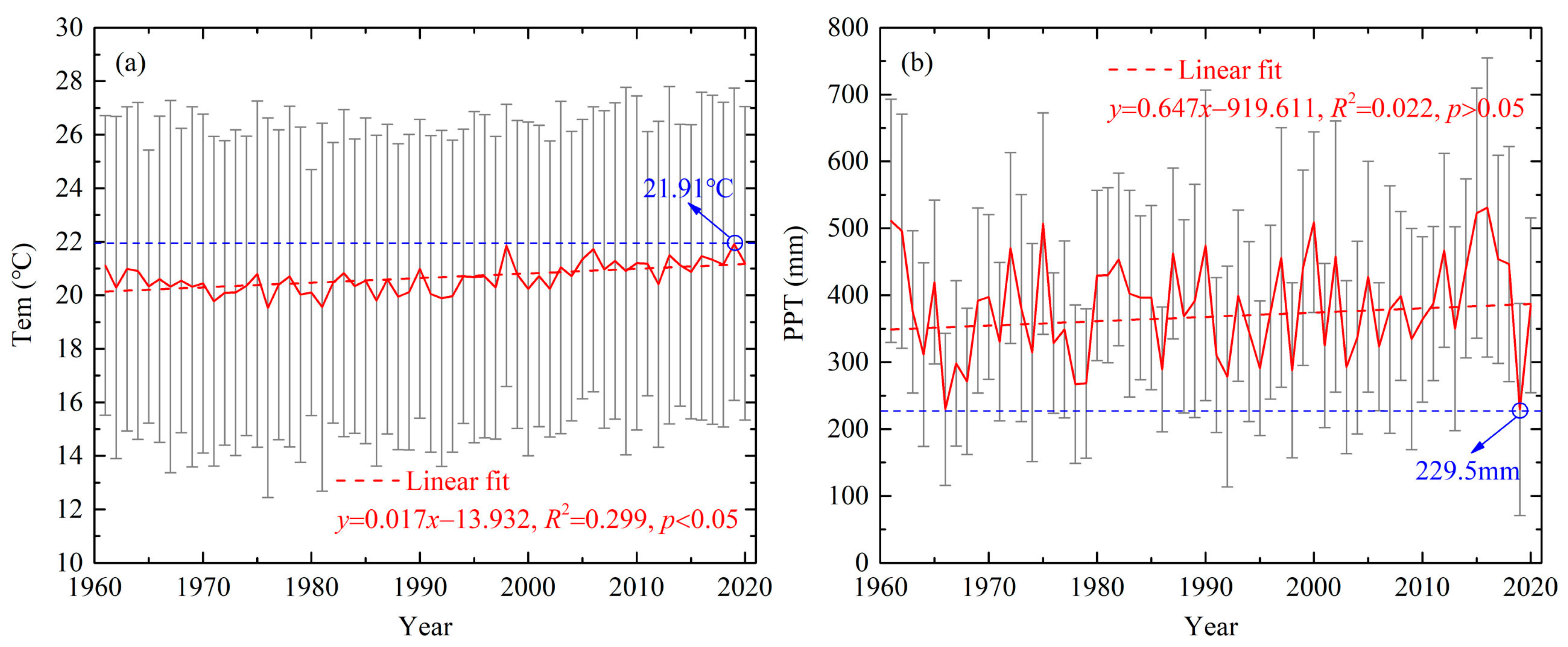
2.2.1. Meteorological Data

The meteorological datasets adopted in this research were the newest routine meteorological observation data from 545 weather stations in the middle and lower reaches of the Yangtze River during 1961–2020, which were provided by the China Integrated Meteorological Information Sharing System (CIMISS) of the China Meteorological Administration (CMA). The datasets include daily average air temperature (Tem, °C) and precipitation (PPT, mm). The annual (monthly) mean Tem and annual (monthly) mean accumulative PPT for analysis were obtained by averaging and summing the daily data of all meteorological stations in the MLRYR to the annual (monthly) time scale. Quality control of the datasets has already been conducted by the National Meteorological Information Center (NMIC) of CMA.

2.2.2. Soil Moisture Data

The monthly root-zone soil moisture (SMroot) and surface soil moisture (SMsurf) datasets at a 0.25° spatial resolution from the latest version (v3.5) of the Global Land Evaporation Amsterdam Model (GLEAM) (https://www.gleam.eu/, accessed on 21 March 2021) were adopted in this study. The above global datasets are based on satellite and reanalysis data and span a 41-year period from 1 January 1980 to 31 December 2020. Furthermore, the datasets were validated in the field across a wide range of ecosystems [29,30].

2.2.3. Standardized Precipitation Evapotranspiration Index (SPEI) Data

The near real-time information about drought conditions at the global scale with a 1° spatial resolution and a monthly time resolution offered by the SPEI Global Drought Monitor was employed to analyze the spatiotemporal patterns of short-term meteorological drought and identify drought events (https://spei.csic.es/, accessed on 18 September 2021). The near real-time character of the SPEI Global Drought Monitor makes it the most suitable for drought monitoring and early warning purposes [31]. Due to the fact that the SPEI with 3 months or more time scales can better reflect the severity and duration of the agricultural drought, the 3-month SPEI (SPEI03) was adopted here. The specific ranking division standard is shown in Table 1.

2.2.4. GOSIF Data

The GOSIF datasets (W·m−2·μm−1·sr−1) consolidated the discrete Orbiting Carbon Observatory-2 (OCO-2) SIF soundings, remote sensing data from the Moderate Resolution Imaging Spectroradiometer (MODIS), and meteorological reanalysis data, with high spatial and temporal resolutions (i.e., 0.05° spatial resolution and 8 day, monthly and annual temporal resolution) [32]. The GOSIF has finer spatial resolution, globally continuous coverage, and a much longer record (from March 2000 to December 2020) obtained from the website (http://data.globalecology.unh.edu/data/GOSIF_v2, accessed on 20 April 2021). At present, GOSIF is useful for assessing terrestrial photosynthesis and ecosystem function and benchmarking terrestrial biosphere and Earth system models. In this study, the 0.05° monthly GOSIF data were employed to examine the performance of SIF in drought monitoring and the relationship between SIF and GPP.

2.2.5. MODIS Data

The MODIS products, including Normalized Difference Vegetation Index (NDVI), Enhanced Vegetation Index (EVI), Near-infrared Reflectance (NIR), Land Surface Temperature (LST °C), Land Cover type (LC), and Gross Primary Productivity (GPP, gC·m−2·month−1) were adopted in this research (https://e4ftl01.cr.usgs.gov/, accessed on 10 June 2021). NDVI, EVI, and NIR were monthly data with 0.05° of spatial resolution from the MOD13C2 product. LST was monthly data with 0.05° of spatial resolution from the MOD11C3 product. LC based on the International Geosphere-Biosphere Programme (IGBP) classification scheme is an annual dataset with 500 m resolution from the MCD12Q1. GPP was an 8-day data with 500 m of spatial resolution from the MOD17A2H product. The monthly GPP data with 0.05° spatial resolution used in this study were synthesized, converted from 8-day data, and weighted based on the number of days in each month [33]. Moreover, the Near-infrared Reflectance of Vegetation (NIRv) adopted in this study is obtained by multiplying NDVI and NIR [34].

2.2.6. Photosynthetically Active Radiation (PAR) Data

The monthly Photosynthetic Active Radiation (PAR) datasets with 1° spatial resolution were obtained from the Cloud and Earth’s Radiant Energy System (CERES) at NASA Langley Research Center. The CERES datasets provide long-term continuous (from March 2000 to present) global radiative fluxes to examine the radiation budget of the Earth’s surface. Here, we adopted the PAR in Synoptic Top-of-Atmosphere (TOA) and Surface Fluxes and Clouds (SYN) Edition 4.1 (https://ceres.larc.nasa.gov/order_data.php, accessed on 6 July 2021). The total PAR is the sum of the surface direct and diffusive PAR under all sky conditions [35].

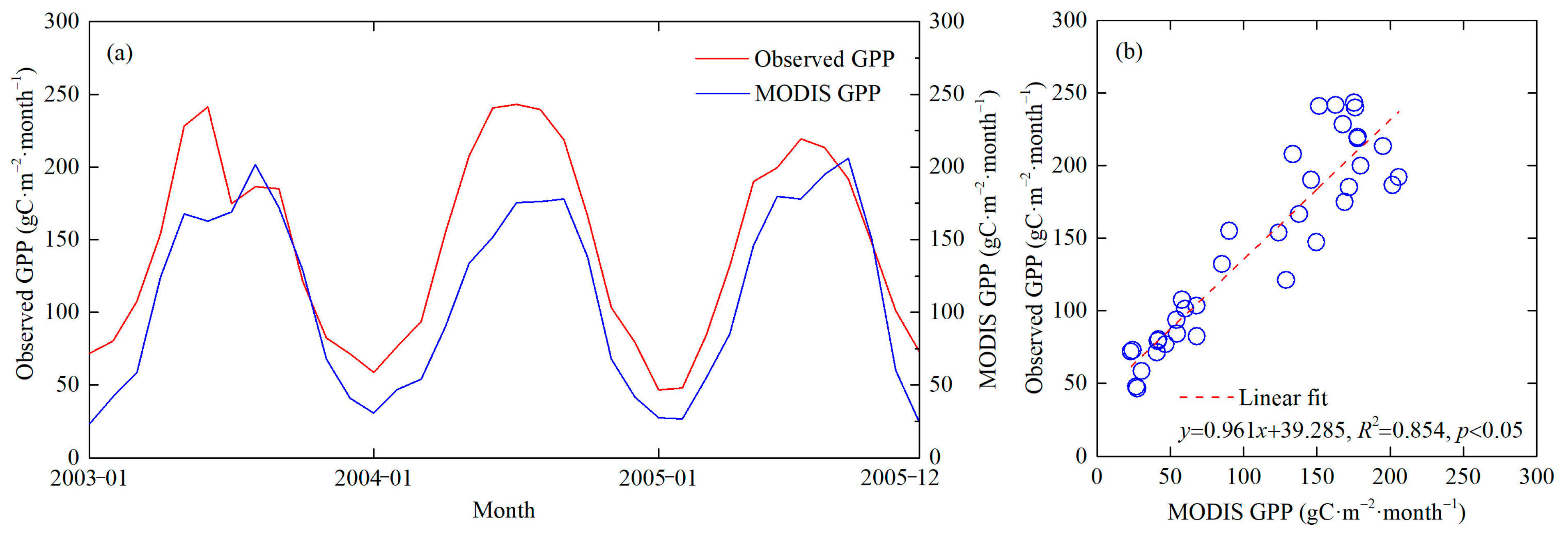
2.2.7. Flux Tower Observation

The Qianyanzhou flux observation station (115.07°E, 26.74°N) was located in Qianyanzhou Red Soil Hilly Agricultural Comprehensive Development Experimental Station of China Ecological Research Network; the micrometeorological observation tower was established in August 2002. The underlying surface slope of the station is between 2.8° and 13.5°, and the forest coverage rate around the tower is more than 90%. GPP observed by the eddy covariance method in the Qianyanzhou ecosystem observatory (Figure 1a) was employed to verify the reliability of MODIS GPP data and explore the correlation between GPP and SIF. The datasets are available monthly during 2003–2005 (http://www.chinaflux.org/index.aspx, accessed on 9 September 2021).

2.3. Methods

2.3.1. Unification of Data Spatiotemporal Resolution

The resolutions of different datasets used in this study varied in spatial and temporal scales. To minimize the errors caused by the mismatch in spatial and temporal resolution, we unified all variables at 0.05° spatial resolution and monthly temporal resolution to maintain consistency with GOSIF data resolution. ArcGIS 10.7 software was used to interpolate the monthly mean air temperature and accumulated precipitation data to 0.05° grid points to match GOSIF for further collaborative analysis.

2.3.2. Standardized Anomaly Index

In order to obtain signals related to water stress, we calculated the spatial distribution of standardized anomalies of each variable at the pixel level in this study [8,33,36]. The pixel (i, j) values of 2019 are compared with the average pixel (i, j) values for the period 2011–2020, and then standardized according to their standard deviation (SD). The specific calculation formula is as follows:
Var 2019   anomaly ( i , j ) = Var 2019 ( i , j ) mean ( Var 2011 2020 ( i , j ) ) SD ( Var 2011 2020 ( i , j ) )
where Var 2019   anomaly ( i , j ) denotes the standardized anomaly of the pixel (i, j) in 2019; Var 2019 ( i , j ) denotes the original value of pixel (i, j) in 2019; mean ( Var 2011 2020 ( i , j ) ) denotes the mean value of pixel (i, j) during 2011–2020; SD ( Var 2011 2020 ( i , j ) ) denotes the standard deviation of pixel (i, j) during 2011–2020. The calculated results indicate the degree to which each month of the drought year (2019) deviates from its associated multi-year (2011–2020) average, representing the drought conditions for each pixel.

2.3.3. Trend and Correlation Analysis

In this study, the following linear equation was used to evaluate the change trends of meteorological factors, VIs, GOSIF, and GPP during the research period:
y = a x + b  
where y is the annual trend of each variable; x is the year; a and b are the slope and intercept, respectively; a positive value of a indicates an increasing trend, while a negative value indicates a decreasing trend. A significance level (p) of 0.05 was used for linear trend analysis and the significance level represents the confidence level of the trend value.
In order to explore the correlation between two indicators, Pearson correlation analysis was used to calculate the correlation coefficient and test the corresponding significance [37]. The specific calculation formula is as follows:
c o r r ( X , Y ) = i = 1 n ( X i X ¯ ) ( Y i Y ¯ ) i = 1 n ( X i X ¯ ) 2 i = 1 n ( Y i Y ¯ ) 2  
where c o r r ( X , Y ) is the Pearson correlation coefficient; X i and Y i are the ith number in X and Y , respectively; X ¯ and Y ¯ are the mean values of X and Y , respectively. The Pearson correlation coefficient is between −1 and 1.

3. Results

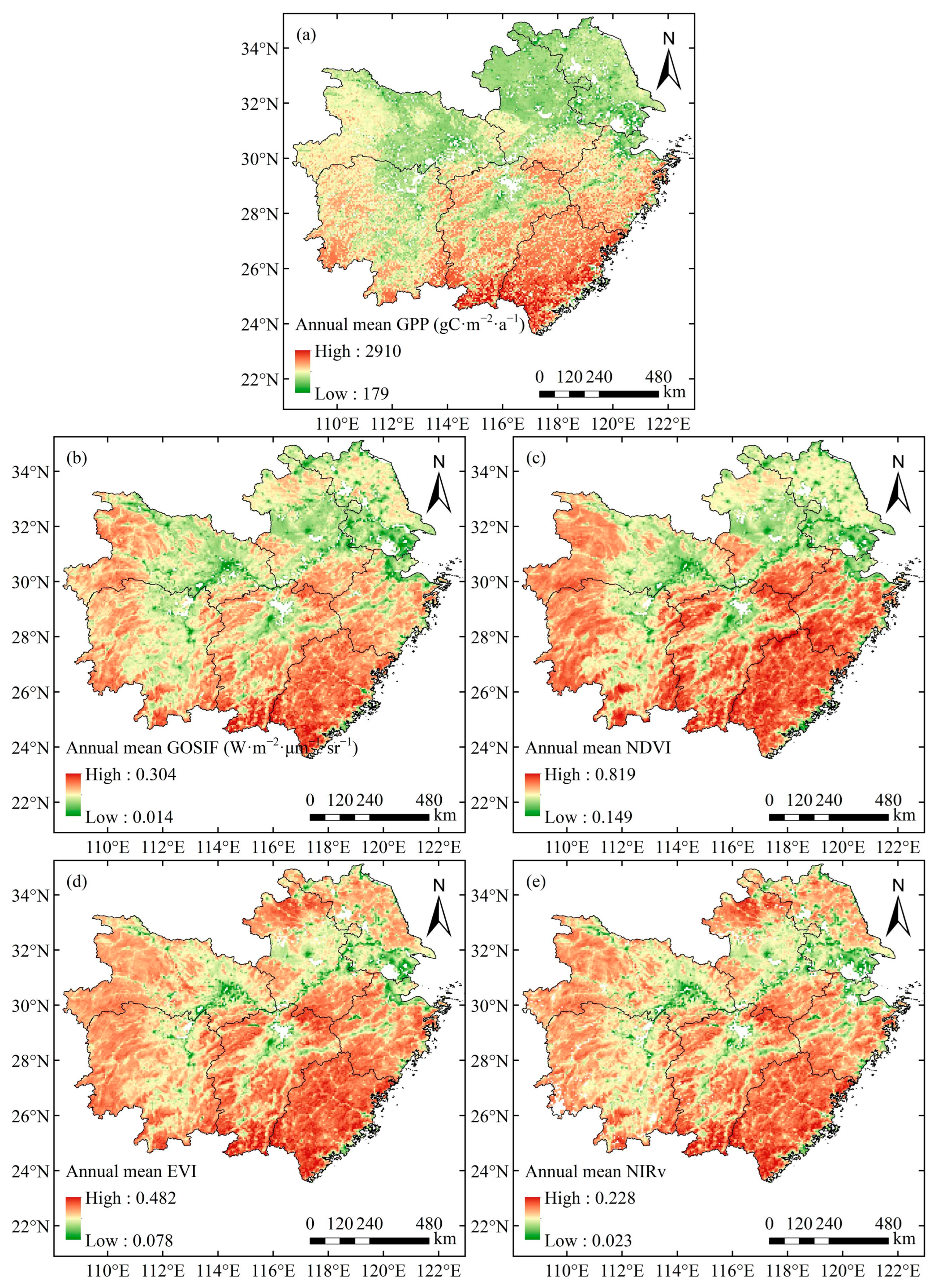
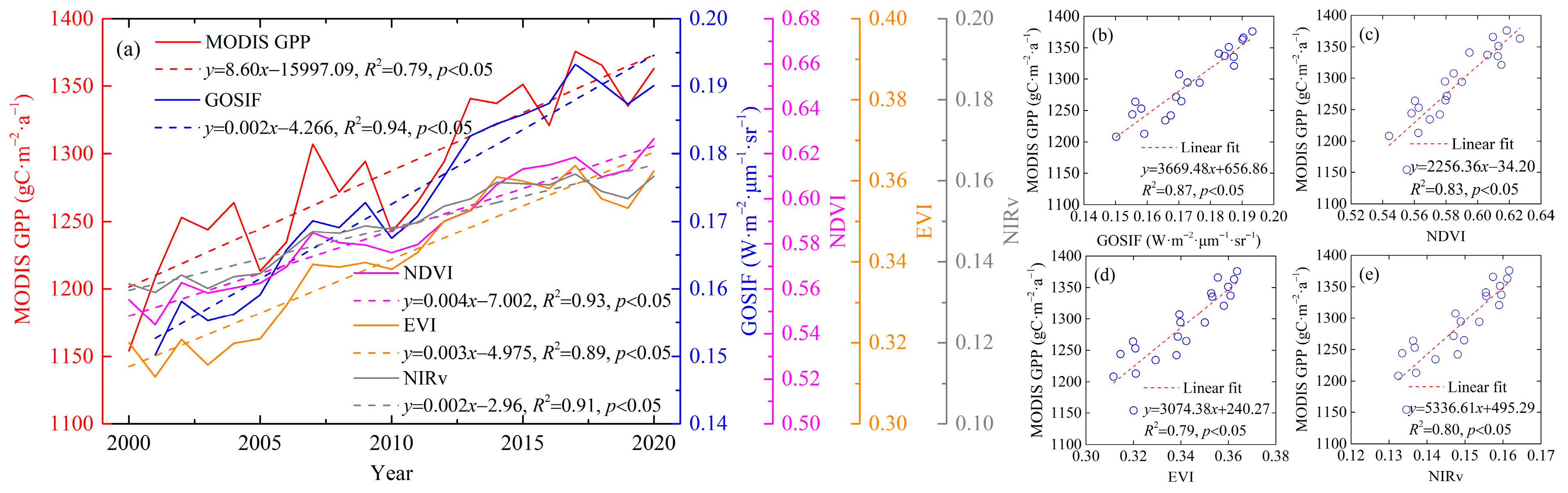
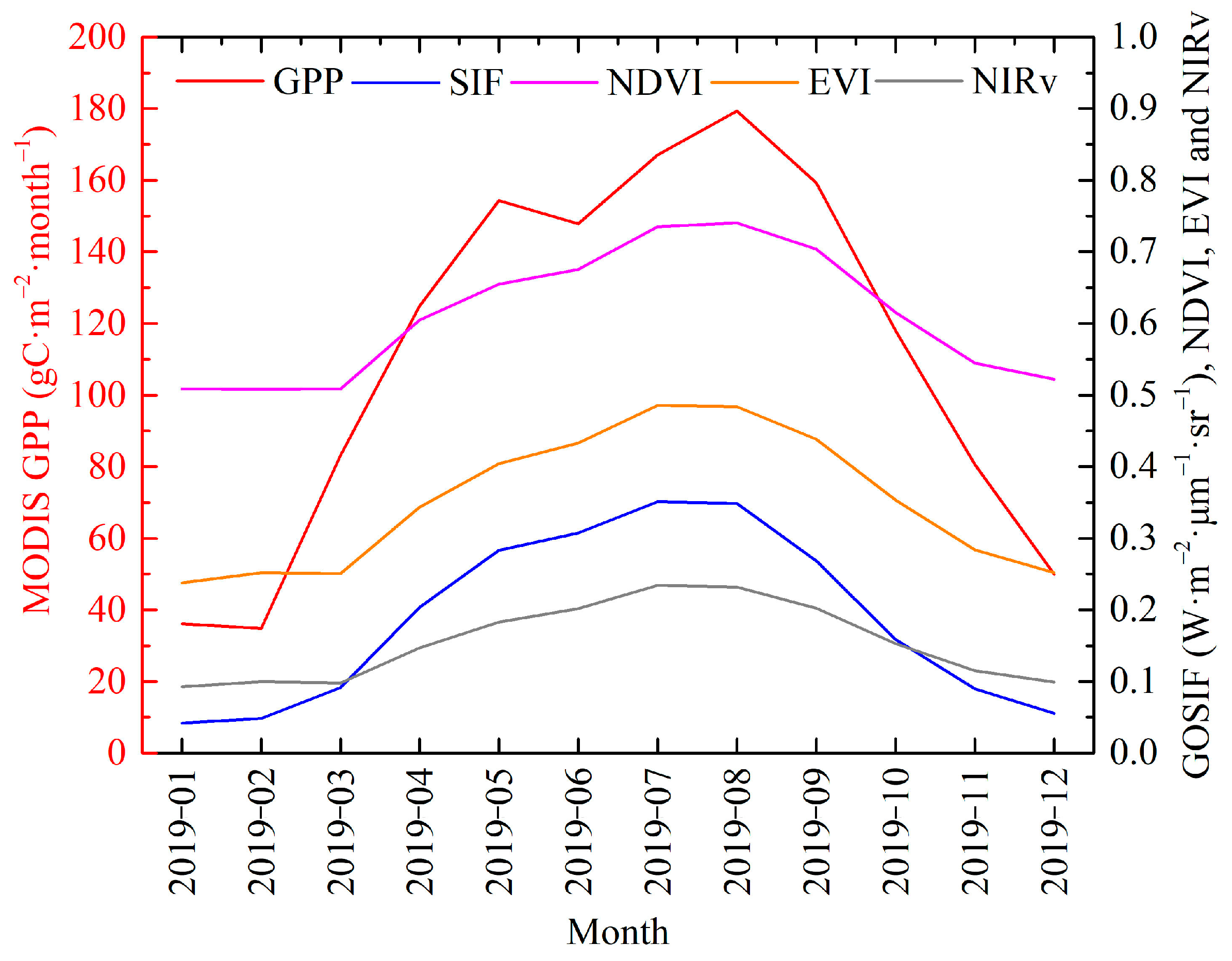
3.1. Spatial–Temporal Variations of GPP, GOSIF, and VIs during 2000–2020

To investigate the effects of drought on vegetation GPP, firstly, we verify the applicability of MODIS GPP product data in the MLRYR by adopting the monthly observed GPP datasets from the Qianyanzhou flux tower during 2003–2005. As shown in Figure 2a, the monthly observed GPP and MODIS GPP exhibited a consistent variation trend, and the MODIS GPP was generally underestimated, especially in 2004. In addition, the effect of scattering fitting between the observed GPP and MODIS GPP is satisfactory, with the R2 value of 0.854 and the p-value less than 0.05 (Figure 2b). The above phenomena manifested that the overall accuracy of MODIS GPP product data is high and can effectively reflect the GPP variation in this region.
To explore the correlation between GPP and GOSIF, NDVI, EVI, and NIRv, the spatial characteristics of these variables during 2000–2020 are displayed in Figure 3. As shown in Figure 3, the annual mean GPP exhibited a gradually decreasing trend from south to north. The spatial difference is evident, with the high values mainly distributed in forests and grasslands. Although GOSIF, NDVI, EVI, and NIRv showed similar spatial distribution characteristics to GPP, the spatial differences between these factors were still apparent. For example, the values of EVI and NIRv were high in the northern parts of Jiangsu and Anhui provinces; the spatial difference of NDVI in the central and southern regions was not noticeable, and there was no gradual change. Moreover, the linear fitting R2 between GPP and SIF, NDVI, EVI, and NIRv at pixel scale is 0.681, 0.676, 0.590, and 0.548, respectively, with all p-values less than 0.05; therefore, the spatial distribution characteristics of GOSIF and GPP are most similar by comparison.
Moreover, as shown in Figure 4a, the GPP, GOSIF, NDVI, EVI, and NIRv all exhibited significant increasing trends during the past 21 years, with the change rate of 8.60 gC·m−2·a−2, 0.002 W·m−2·μm−1·sr−1·a−1, 0.004 a−1, 0.003 a−1, and 0.002 a−1, respectively. In terms of the changing trend, the GOSIF was also closest to the GPP. To reveal the correlation between GPP and other VIs, the annual scatter fittings between GPP and GOSIF, NDVI, EVI, and NIRv are displayed in Figure 4b–e. The relationship between GPP and each vegetation index exhibited linear correlation; the corresponding R2 values were 0.87, 0.83, 0.79, and 0.80, respectively, with all p-values less than 0.05, which verified that the GOSIF is most correlated with GPP on an annual basis time scale.
The monthly GPP, GOSIF, NDVI, EVI, and NIRv exhibited evident interdecadal variation characteristics (Figure 5a). In addition, the correlation between monthly GPP and GOSIF, NDVI, EVI, and NIRv during 2000–2020 presented polynomial distribution (Figure 5b–e). The fitting R2 are 0.976, 0.891, 0.948, and 0.945, respectively, which further verified that the GOSIF is also most correlated with GPP on the monthly time scale.

3.2. Spatial–Temporal Patterns of Standardized Anomalies of Drought Indices during the 2019 Drought

To reflect the intensity of the drought process in the MLRYR, the average Tem and accumulated PPT among all meteorological stations from August to November in the past 60 years were analyzed. As shown in Figure 6a, the Tem exhibited a significant upward trend (0.017 °C a−1, p < 0.05), with a significant downward trend before 1990 and a significant upward trend after that. In 2019, the Tem reached 21.91 °C, slightly higher than in 1998—the highest in the past 60 years. In addition, unlike Tem, PPT generally showed a nonsignificant fluctuation upward trend (0.647 mm·a−1, p > 0.05) during 1961–2020; however, in 2019, PPT was only 229.5 mm, slightly lower than 1966, with the lowest in the past 60 years (Figure 6b). High Tem and less PPT led to this typical continuous drought in 2019 summer and autumn in this region.
To further reveal the intensity and scope of the 2019 drought event process, seven drought indexes, namely PPT, SMsurf, SMroot, SPEI, Tem, LST, and PAR, were selected for this research. Moreover, in order to explore the drought process more specifically, we extended the study period by one month, namely from July to December 2019. The spatial–temporal characteristics of standardized anomalies of each index from July to December 2019 are analyzed in Figure 7. As shown in Figure 7a, except for July, PPT in other months of 2019 was all below the averages during 2011–2020. From July to September, the monthly average of PPT showed a significant downward trend in 2019. It reached a low point in September (33.1 mm), where the difference between the monthly average of 2019 and that during 2011–2020 was the largest (79.1 mm). Then, the PPT increased slightly in October and reached its lowest point in November (26.6 mm). After that, the PPT increased steadily and was close to the average level during 2011–2020 in December (46.7 mm). In Figure 7b,c, the SMsurf and SMroot presented similar variation characteristics. The soil moisture was slightly higher than the average in July, then exhibited a significant decreasing trend and reached the lowest point in November (0.287 m3·m−3). The difference between the monthly average of 2019 and that during 2011–2020 was the largest (0.078 m3·m−3). After that, the soil moisture increased somewhat in December, especially in the SMsurf. As shown in Table 1, a similar phenomenon can also be detected from SPEI in Figure 7d, especially from September to December; the SPEI values were lower than 0.5 and reached the lowest in November (−1.66).
Contrary to other variables, as can be seen in Figure 7e,f, the Tem and LST in July of 2019 were both below the multi-year average during 2011–2020; however, the Tem and LST are significantly higher than the multi-year average in other months. Similar change characteristics could also be found in PAR except for October, while in October, the PAR in 2019 is virtually indistinguishable from the 2011–2020 average (Figure 7g).
Figure 8 presents the standardized anomalies of PPT, SMsurf, SMroot, SPEI, Tem, LST, and PAR spatially. The standardized anomaly of SPEI showed a similar variation characteristic as that on the temporal scale (Figure 7d). During July–August, the negative SPEI standardized anomalies were mainly distributed in the northern part of MLRYR, namely HB, AH, and JS provinces. From September to November, the negative standardized anomalies of SPEI gradually expanded from north to south and almost the entire area. In December, the location of the negative SPEI standardized anomaly has shrunk. In July, the negative PPT standardized anomaly area was mainly distributed in the northern part of MLRYR, while in August and September, the negative area gradually expanded to the whole location. In October, the negative PPT standardized anomaly area decreased and was mainly distributed in the central region. In November, the negative PPT standardized anomaly area covers almost the entire area. In December, the precipitation increased obviously. The distribution characteristics of SMsurf and SMroot were consistent with that of SPEI, especially the SMsurf, which is due to the fact that the negative area tends to shrink towards the center region. The spatial distributions of Tem and LST were consistent and matched with the distribution characteristics of soil moisture. The spatial distribution trend of the standardized anomaly of PAR is most compatible with PPT. In addition, it is noteworthy that, although both PPT and SPEI indicated that the drought trend eased in December, soil moisture and Tem data remained at abnormal levels.

3.3. Spatial–Temporal Patterns of Standardized Anomalies of GOSIF and VIs during the 2019 Drought

As shown in Figure 9, the monthly variation trends of GOSIF, NDVI, EVI, and NIRv were similar and gradually decreased from July to December; however, on the temporal scale, the differences between the monthly average of 2019 and that of 2011–2020 averages for SIF and each vegetation index are not significant. This phenomenon may be due to the averaging of high and low values across the region. Considering the complexity of regional drought, the comparison of monthly average changes between 2019 and 2011–2020 from July to December still cannot reflect the intensity of the drought occurrence in 2019. Thus, it is necessary to explore the standardized spatial anomalies of SIF and vegetation indices.
To further reveal the impact of drought on vegetation in 2019, the spatial distributions of the standardized anomalies of GOSIF, NDVI, EVI, and NIRv from July to December 2019 are displayed in Figure 10. In July, the negative anomaly of GOSIF was mainly distributed in the southern part of the MLRYR; however, the corresponding PPT, SPEI, SMsurf, and SMroot were positive. In addition, the negative anomalies of NDVI, EVI, and NIRv exhibited relatively sparse distribution, especially the NDVI. In August, the negative anomaly of GOSIF was mainly distributed in Hubei province. Unlike GOSIF, the negative anomaly region of NDVI in Jiangxi province was apparent.
Moreover, the negative anomaly areas of EVI and NIRv were enlarged to most of Hunan province, northern Fujian Province, central and southern Zhejiang, and Anhui province. The spatial negative anomaly distribution of GOSIF, NDVI, EVI, and NIRv is generally consistent. In September, the hostile anomaly areas of GOSIF, NDVI, EVI, and NIRv were mainly distributed in Hubei, Hunan, and Jiangxi provinces. In October, the negative anomaly areas between GOSIF and NDVI and EVI and NIRv were consistent; however, in November, the negative anomaly area of GOSIF had been reduced, which was mainly distributed in the central and northeastern regions of MLRYR. Unlike GOSIF, the negative anomalies of NDVI, EVI, and NIRv were still severe; the distribution characteristics were similar to those of GOSIF. In December, the negative anomaly area of GOSIF was further reduced, while NDVI, EVI, and NIRv decreased slowly and were mainly distributed in central and southern Anhui province, most parts of Jiangxi province, western Zhejiang and Fujian provinces, and the eastern parts of Hubei province.

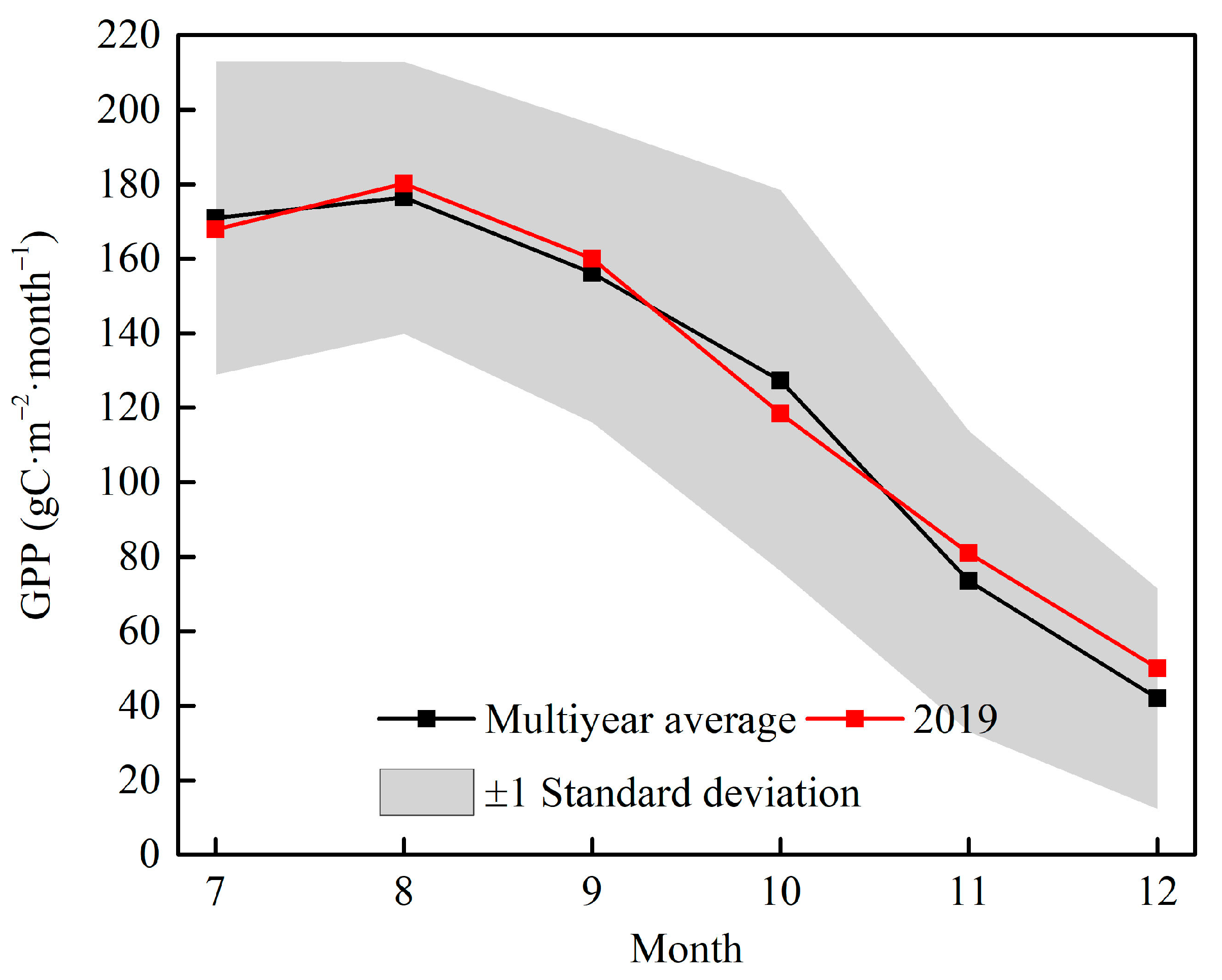
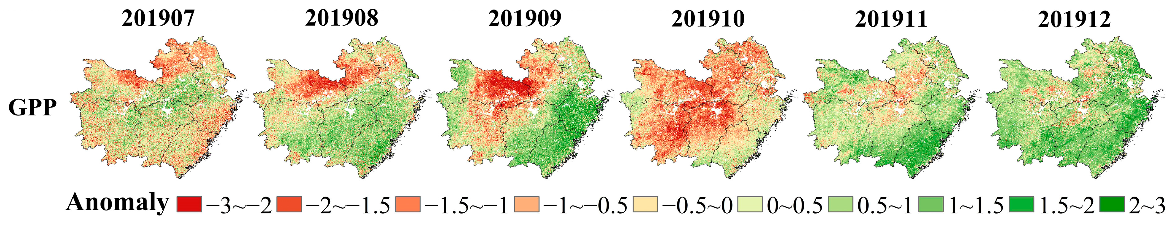
3.4. Spatial–Temporal Patterns of Standardized Anomalies of GPP during the 2019 Drought

As shown in Figure 11, the monthly variations of GPP during July–December 2019 were consistent with GOSIF and VIs in Figure 9, and generally exhibited a gradually decreasing trend. In addition, the GPP in July and October of 2019 was slightly lower than the monthly average during 2011–2020, especially in October (the difference is 8.8 gC·m−2·month−1); however, in other months of 2019, the GPP was higher, especially in November and December (the differences are 7.3 gC·m−2·month−1 and 8.2 gC·m−2·month−1, respectively).
Figure 12 shows the spatial distributions of the standardized anomalies for GPP from July to December 2019. We found that the negative GPP anomaly was more evident during August–October. In August, the region with a negative GPP anomaly was mainly distributed in the northern part of the MLRYR, especially the central and eastern parts of Hubei province and the northern part of Anhui province. In September, the negative anomaly areas were more prominent and had extended to some areas of Hunan and Jiangxi Provinces. In October, most regions of MLRYR exhibited negative anomalies, especially Hubei, Hunan, Jiangxi, Anhui, and Jiangsu provinces; however, the negative anomaly areas shrank gradually in November and December, especially in December. Combining with Figure 10, we found the distribution characteristics of the GPP standardized anomaly during the drought in 2019 are more similar to that of GOSIF, especially obvious in November and December.

3.5. Spatial Consistency between MODIS GPP and GOSIF, NDVI, EVI, and NIRv during the 2019 Drought

To further reveal the correlation between MODIS GPP and GOSIF, NDVI, EVI, and NIRv during the 2019 drought event, we analyzed the spatial consistency between GPP and GOSIF, NDVI, EVI, and NIRv (Figure 13), as well as the spatial consistency between standardized anomalies of GPP and GOSIF, NDVI, EVI, and NIRv (Table 2), respectively. As shown in Figure 13, the linear fitting R2 value between MODIS GPP and GOSIF, NDVI, EVI, and NIRv were 0.742, 0.646, 0.664, and 0.674, respectively; all were positively correlated. Similar to the results in Figure 5, the relationship between MODIS GPP and SIF is also polynomial dependent, while that between GPP and NDVI, EVI, and NIRv were different. As displayed in Table 2, similar to Figure 13, the relationship between standardized anomalies of GPP and SIF, NDVI, EVI, and NIRv at pixel scale was also positively correlated during July–December. In July and October 2019, the NDVI performed better, with R-values of 0.157 and 0.451, respectively. While in other months, SIF performed better, with the linear fitting R-values of 0.341, 0.525, 0.368, and 0.367. The above phenomenon further verified the good spatial consistency between SIF and GPP compared with other VIs and the superior ability of SIF in capturing and quantifying drought-induced GPP losses.

4. Discussion

4.1. Responses of SIF and VIs to Drought

From the change characteristics of SPEI, SMsurf, and SMroot in Figure 7 and Figure 8, the drought still existed in the MLRYR in November and December 2019. Although the drought in December 2019 was alleviated compared with that in November 2019, the standardized anomalies of SPEI and soil moisture were still negative and Tem, LST, and PAR were positive. Correspondingly, the standardized anomalies of NDVI, EVI, and NIRv still changed considerably during November and even December of 2019, while those of SIF did not change significantly (Figure 10). As SIF is a direct probe of photosynthesis, it can capture the physiological state information of vegetation directly. During November–December 2019 and the same period throughout the year in the MLRYR, the vegetation generally entered the senescence stage and its photosynthetic capacity declined. Despite being affected by drought during this period, vegetation senescence information played a dominant role in the SIF signal changes, which resulted in the little anomaly change of regional SIF; however, VIs (e.g., NDVI, EVI, and NIRv) are vegetation greenness indices [38], which are not as closely related to the physiological state of vegetation as SIF and cannot capture the changes of vegetation senescence stage sufficiently; therefore, VIs had an obvious delayed response in monitoring the physiological state of vegetation compared with SIF. This phenomenon is consistent with previous studies [6,7,8,33,39,40]. Moreover, the vegetation was sparse and the leaf area index (LAI) was low during this time period; the VIs were significantly affected by soil background [41], which determined the dominant role of drought in NDVI, EVI, and NIRv changes ultimately. The above explanation could also be responsible for the apparent negative standardized anomalies of NDVI, EVI, and NIRv in central MLRYR. The results were echoed by Wang et al. [15], who pointed out that the decrease in SIF was more significant than that of NDVI during the peak growth period in the Great Plains, while the reduction in NDVI continued and that of SIF eased during the senescence stage. Wang et al. [42] also indicated that SIF is better than NDVI in determining the end date of the vegetation growing season. Moreover, as shown in Figure 14, the relative higher coefficients in September 2019 and the lower coefficients in December 2019 between the standardized anomalies of SIF and those of drought indices can also give a reasonable and quantitative explanation for the responses of SIF and VIs to drought in this study. In general, when vegetation enters the senescence stage gradually in autumn and winter, the VIs better reflect meteorological drought conditions if the drought continues.

4.2. Impacts of Drought on GPP

This study investigated the MODIS GPP product accuracy by employing the monthly observed GPP datasets from the Qianyanzhou flux tower. The overall accuracy of MODIS GPP product data is good. Further studies should also combine with other GPP products [43,44] (e.g., the Global LAnd Surface Satellite (GLASS) GPP [45] and the Fluxcom GPP [46]) to explore the regional GPP variation accurately. Furthermore, it is notable that in Figure 12, the negative standardized anomalies areas for GPP during November and December in 2019 decreased significantly, which was consistent with that of GOSIF, while the standardized anomalies areas of VIs are still significant (Figure 10). This phenomenon indicated that the responsibility of NDVI to short-term precipitation is limited, which may lead to delayed expression of vegetation production recovery. As shown in Figure 7d, the most severe meteorological drought occurred in November 2019; while the reduction in GPP was not noticeable (Figure 12), this phenomenon could be explained by the difference between meteorological drought and agricultural drought. Although the VIs can indicate the agricultural drought potentially [47,48,49], considering the reduction in VIs was significant in November and December, which was not found for GOSIF, the actual agricultural drought that emphasizes yield reduction, or GPP losses may be less severe in the MLRYR [15]. Moreover, Liu et al. [24] also reported that the well-known 2019 drought event that occurred in the MLRYR had a much less severe impact on vegetation than expected; this is mainly due to the lack of Pre, leading to an increase in sunshine and heat resources, which in turn improved crop growth in most areas; therefore, compared with VIs, SIF can better monitor the vegetation’s physiological state changes (e.g., senescence) and GPP variations even when suffering from agricultural drought. In addition, due to the fact that the crop water demand (e.g., rice and wheat) in MLRYR can be satisfied by irrigation when drought occurs [24,50], the mitigation of drought effects on crop GPP by irrigation and groundwater storage [15] and the impacts of climatic impacts of irrigation on crop growth [50,51] deserve more attention and need further research in this region.

4.3. Relationship between GPP and SIF

This research verified that the GOSIF is most correlated with GPP compared with VIs in both spatial and temporal time scales and that the relationship between annual GOSIF and GPP is linear (Figure 4). A similar result was consistent with Ma et al. [22], who reported that the Vegetation Photosynthesis Model (VPM)-based GPP (namely GPPVPM) is compatible with GOME-2 SIF at multiple spatial–temporal scales in China, and the monthly GPPVPM and SIF showed a significant positive linear correlation in most areas. The linear correlation relationship provides a theoretical basis for the subsequent estimation of GPP by SIF at sites or ecosystem levels [52]; however, the correlation between monthly GOSIF and GPP during 2000–2020 presented a polynomial distribution in the MLRYR (Figure 5) and the polynomial fitting R2 is as high as 0.976. Similar results could be found in Figure 13a. Paul-Limoges et al. [53] found that SIF was more susceptible to the environmental conditions (e.g., drought and heat stresses, incoming photosynthetic photon flux density, vegetation types, etc.) than GPP; this is worthy of further study, aiming to provide the possibility of reliable estimation of GPP from the perspective of remote sensing observations. Wohlfahrt et al. [54] studied that SIF cannot track GPP variation well during a short-term heatwave in ENF, further revealing that the nonlinear and complex SIF–GPP relationship exists at different time scales. The research of He et al. [55] showed the broken linear SIF–GPP relationship at high-light levels since the GPP tends to saturate while SIF still increases, especially for C3 crops. Kim et al. [56] also reported a strongly nonlinear relationship (hyperbolic regression function) between GPP and SIF in a temperate Evergreen Needleleaf Forest (ENF) at daily and seasonal time scales, which was mainly due to the different physiological mechanisms. In addition, canopy structure and vegetation coverage of diverse communities may be the main influencing factors of spatial heterogeneity of the SIF–GPP relationship [36]. Huang et al. [57] indicated that the tides play an important role in regulating SIF–GPP relationships. Due to the tides, inundation attenuated the role of plant physiology and canopy structure in explaining the relationship between SIF and photosynthesis, thus negatively affecting SIF-based GPP estimates. Martini et al. [58] revealed that the heatwave reversed the photosynthesis–fluorescence relationship at canopy and leaf scales, and the highly non-linear relationship between GPP and SIF is formed by Non-Photochemical Quenching (NPQ), a dissipative mechanism that prevents the adverse effects of high light intensity. To preliminarily investigate the nonlinear relationship between monthly SIF-GPP in this research more clearly, the monthly GPP, SIF, NDVI, EVI, and NIRv variations in 2019 were analyzed, as shown in Figure 15; we see that the monthly variation characteristics of SIF, NDVI, EVI, and NIRv were similar. At the same time, the GPP increased significantly from February to May and decreased considerably from September to December, which was different from that of SIF and VIs. This phenomenon might be responsible for the nonlinear relationship between GPP and SIF. Moreover, we found a polynomial relationship between monthly GPP and SIF in both drought (2019) and non-drought years; however, the findings of Song et al. [36] claimed a constant SIF–GPP relationship under both drought and non-drought conditions, although the drought stress increased the spatial heterogeneity of the SIF–GPP relationship; therefore, it will be uncertain to explore the influence of environmental stress on the GPP–SIF relationship only from a satellite remote sensing scale. Furthermore, Liu et al. [59] found that the nonlinear relationship between SIF and GPP generally existed in eight major biomes (ENF, EBF, DBF, MF, SHR, SAV, GRA, and CRO), and the exponential regression model was the best method to capture the nonlinear relationship between SIF and GPP at the site level. Thus, significant errors will exist in estimating GPP or evaluating GPP loss caused by drought at regional scale only by relying on a simple fixed linear model between SIF and GPP [6,44]. In addition, whether different GPP products and SIF inversion data will affect the SIF–GPP relationship remains to be further studied. Subsequent studies can carry out field crop water stress experiments by adopting the high-resolution fiber optic spectrometer (e.g., QE-PRO spectrometer, Ocean Optics, Inc., Dunedin, FL, USA) and then investigate the effect of environmental stress on the SIF–GPP relationship through more refined experimental observation data.

5. Conclusions

In this research, the performance of SIF and vegetation indexes in monitoring and evaluating the effects of the well-known 2019 drought in the MLRYR on vegetation was compared and analyzed, aiming to provide a decision-making reference for regional drought remote sensing monitoring. The main results are presented as follows:
  • MODIS GPP can reflect the GPP variation in the MLRYR effectively. The GPP, GOSIF, NDVI, EVI, and NIRv all exhibited significant increasing trends during 2000–2020. When compared to VIs, the spatial distribution characteristics of GOSIF and GPP were most similar, and GOSIF was most correlated with GPP in both annual (linear correlation, R2 = 0.87) and monthly (polynomial correlation, R2 = 0.976) time scales.
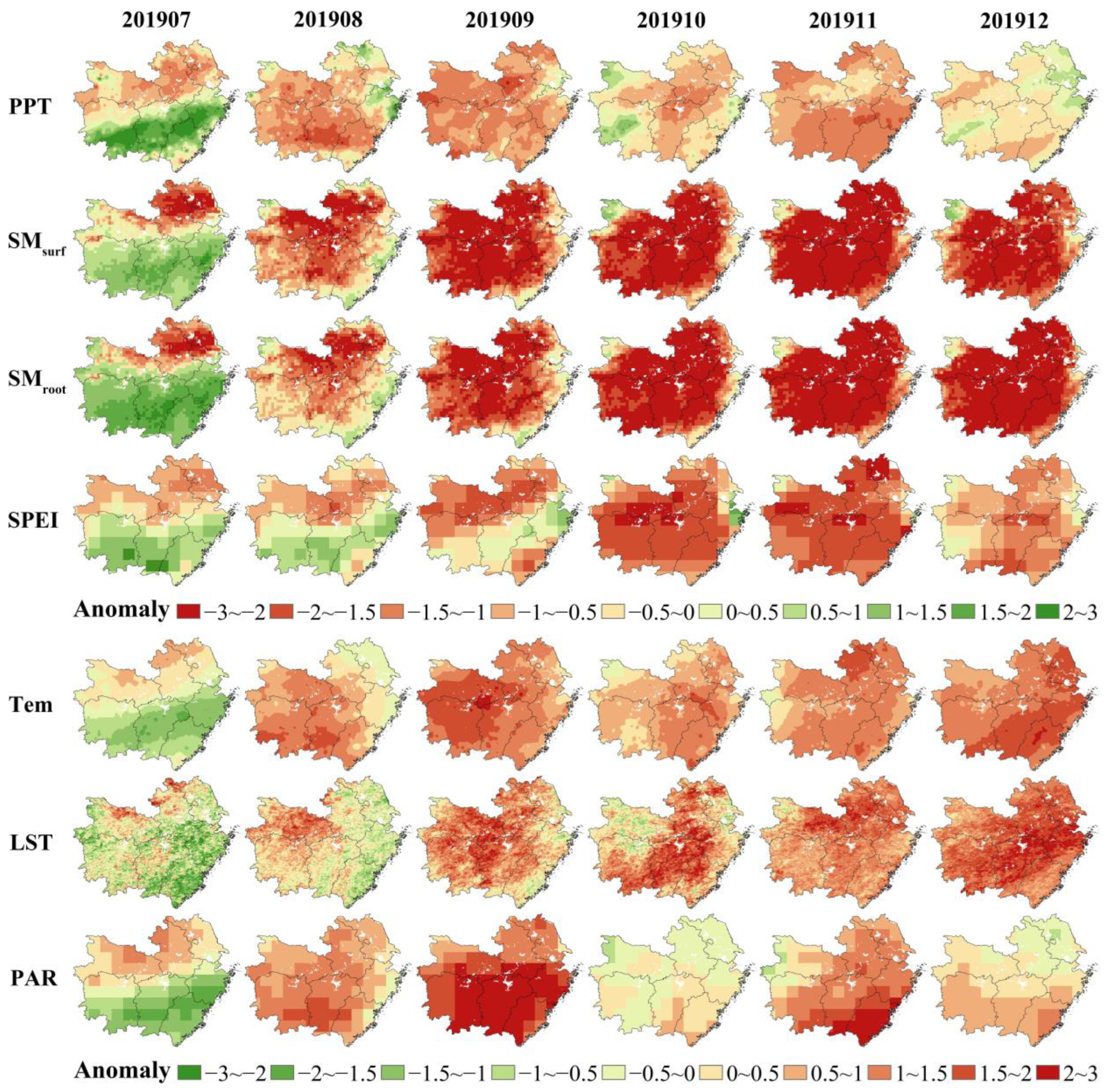
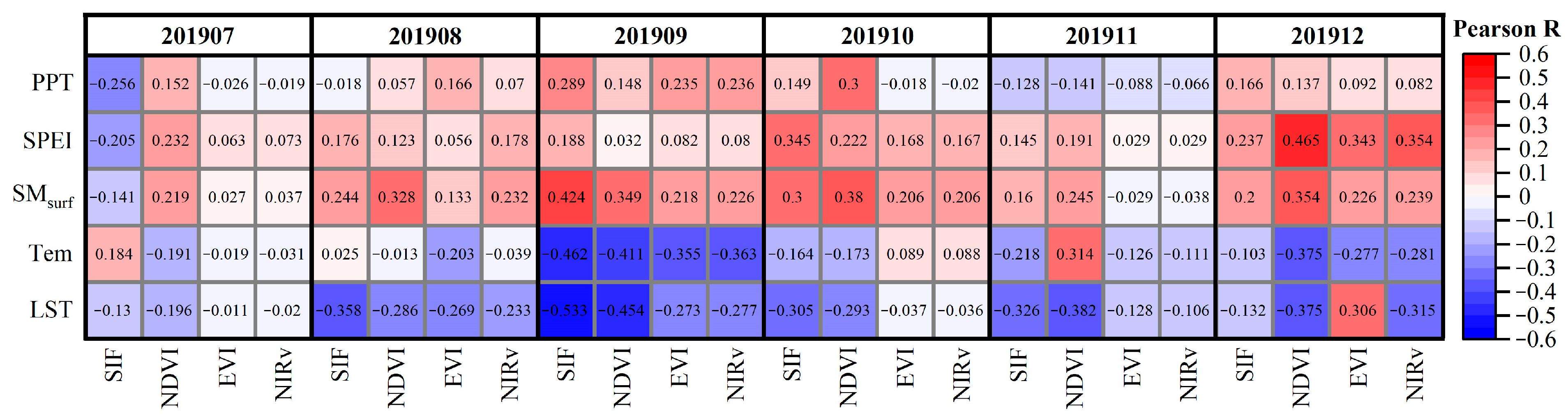
  • From July to December, the PPT, SMsurf, SMroot, and SPEI in 2019 were generally below the averages during 2011–2020 and reached their lowest point in November, while those of Tem, LST, and PAR, on the contrary, were higher. Similar results could also be verified from the standardized anomalies of the above variables on the spatial.
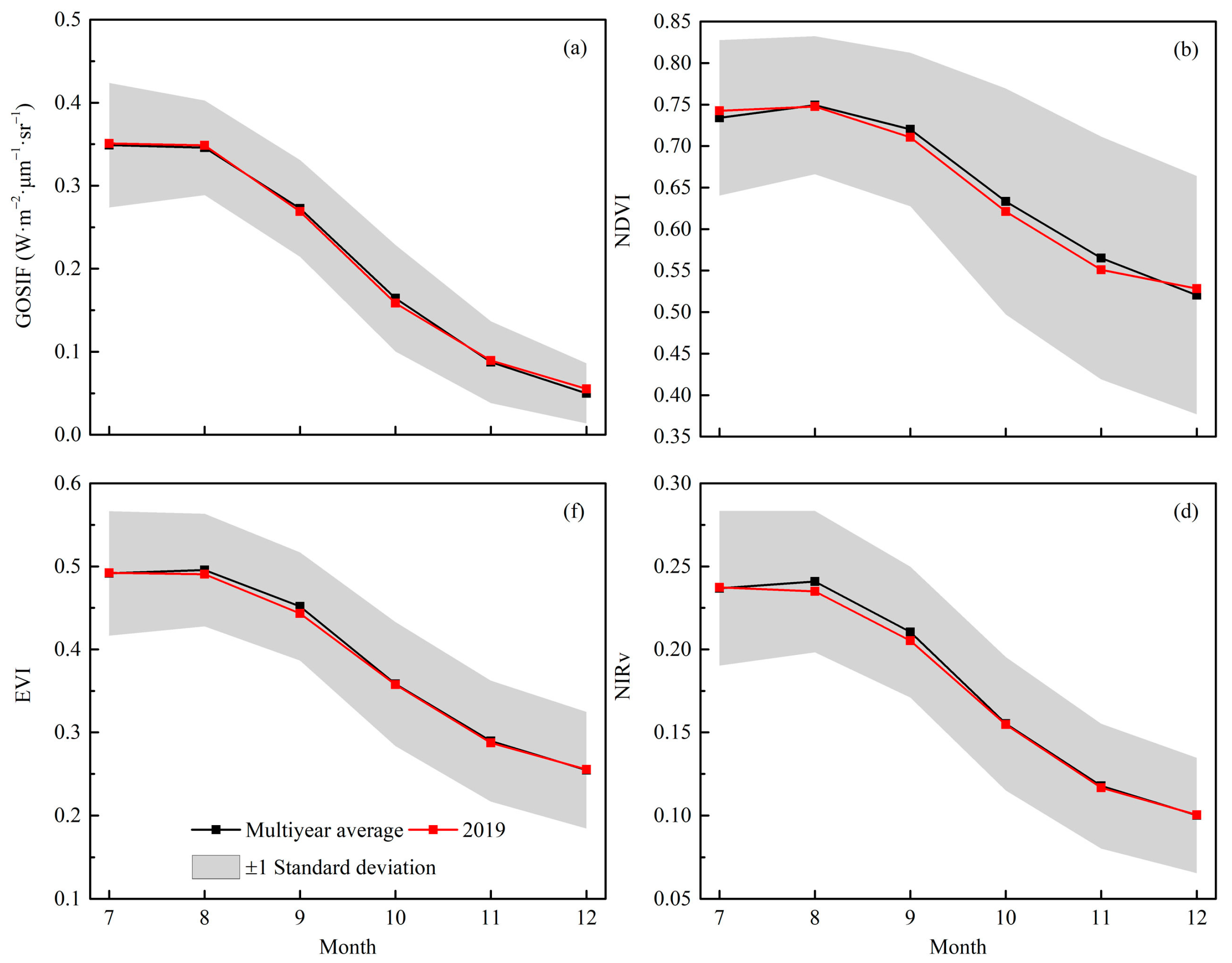
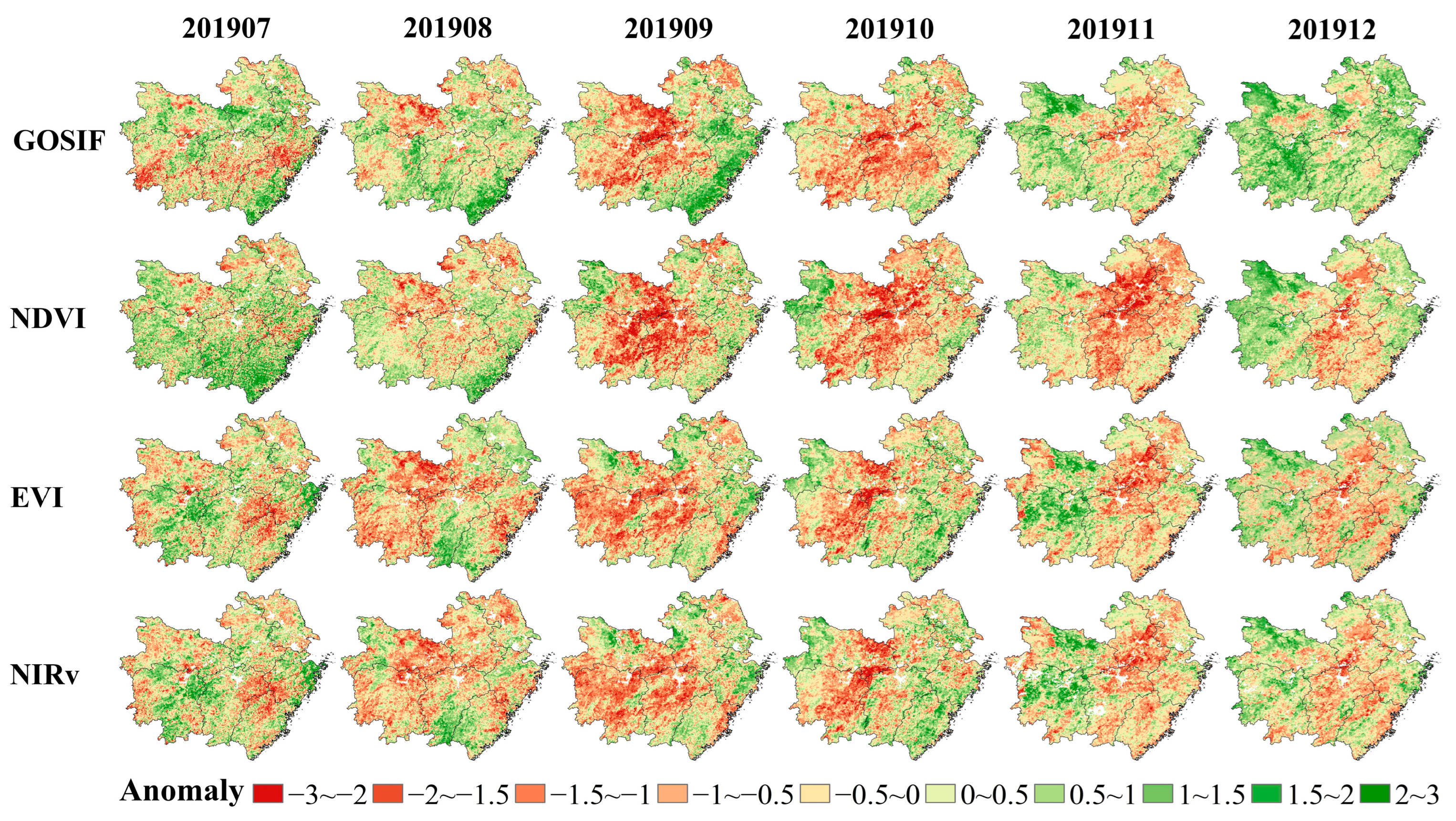
  • The differences between the monthly averages of 2019 and 2011–2020 for SIF and VIs are not significant on a temporal scale. Spatial distributions of standardized anomalies of SIF and VIs were consistent during August–October 2019. In November and December, however, the regional difference in SIF anomaly was small, and that of VIs still changed significantly.
  • When vegetation was entering the senescence stage in November and December, the VIs had an obvious delayed response in monitoring vegetation’s physiological state compared with SIF, while the VIs could better indicate meteorological drought conditions compared with SIF.
  • The distribution characteristic of the GPP standardized anomaly during the 2019 drought was more similar to that of GOSIF, especially obvious in November and December, which exhibited the superior ability of SIF in capturing and quantifying drought-induced GPP losses.
This study revealed that SIF has good performance in drought monitoring at the normal vegetation growth stage and can evaluate drought-induced GPP losses. Subsequent studies should focus on how to bring the above potential into play and then solve the scientific problem of how to apply SIF to monitor and evaluate the intensity of drought events systematically, e.g., the construction of a drought stress fluorescence monitoring index based on SIF.

Author Contributions

Conceptualization, M.L. and R.C.; Software, X.S., P.X., F.N. and C.W.; Validation, M.L., R.C. and X.S.; Formal Analysis, M.L. and R.C.; Data Curation, M.L., R.C., X.S., P.X., F.N. and C.W.; Writing—Original Draft Preparation, M.L. and R.C.; Supervision, M.L. and R.C.; Funding Acquisition, M.L., R.C. and Y.J.; Writing—Review and Editing, Y.J., S.S. and A.R.M.T.I. All authors have read and agreed to the published version of the manuscript.

Funding

This research was funded by the Anhui Provincial Natural Science Foundation (2108085QD157; 1908085QD171), National Natural Science Foundation of China (41905100), National Key Research and Development Program of China (2018YFD0300905), Anhui Agricultural University Science Foundation for Young Scholars (2018zd07), Anhui Agricultural University Introduction, and Stabilization of Talent Fund (yj2018-57).

Data Availability Statement

Not applicable.

Conflicts of Interest

The authors declare no conflict of interest.

References

  1. Tian, F.; Wu, J.; Liu, L.; Leng, S.; Yang, J.; Zhao, W.; Shen, Q. Exceptional Drought across Southeastern Australia Caused by Extreme Lack of Precipitation and Its Impacts on NDVI and SIF in 2018. Remote Sens. 2020, 12, 54. [Google Scholar] [CrossRef] [Green Version]
  2. Zhao, M.S.; Running, S.W. Drought-induced reduction in global terrestrial net primary production from 2000 through 2009. Science 2010, 329, 940. [Google Scholar] [CrossRef] [PubMed] [Green Version]
  3. He, M.; Kimball, J.S.; Yi, Y.; Running, S.; Guan, K.; Jensco, K.; Maxwell, B.; Maneta, M. Impacts of the 2017 flash drought in the US Northern plains informed by satellite-based evapotranspiration and solar-induced fluorescence. Environ. Res. Lett. 2019, 14, 074019. [Google Scholar] [CrossRef] [Green Version]
  4. IPCC. Climate Change 2014: Impacts, Adaptation, and Vulnerability. Contribution of Working Group II to the Fifth Assessment Report of the Intergovernmental Panel on Climate Change; Cambridge University Press: Cambridge, UK, 2014. [Google Scholar]
  5. West, H.; Quinn, N.; Horswell, M. Remote sensing for drought monitoring & impact assessment: Progress, past challenges and future opportunities. Remote Sens. Environ. 2019, 232, 111291. [Google Scholar]
  6. Chen, X.; Mo, X.; Zhang, Y.; Sun, Z.; Liu, Y.; Hu, S.; Liu, S. Drought detection and assessment with solar-induced chlorophyll fluorescence in summer maize growth period over North China Plain. Ecol. Indic. 2019, 104, 347–356. [Google Scholar] [CrossRef]
  7. Liu, L.; Yang, X.; Zhou, H.; Liu, S.; Zhou, L.; Li, X.; Yang, J.; Han, X.; Wu, J. Evaluating the utility of solar-induced chlorophyll fluorescence for drought monitoring by comparison with NDVI derived from wheat canopy. Sci. Total Environ. 2018, 625, 1208–1217. [Google Scholar] [CrossRef]
  8. Wang, X.; Qiu, B.; Li, W.; Zhang, Q. Impacts of drought and heatwave on the terrestrial ecosystemin China as revealed by satellite solar-induced chlorophyll fluorescence. Sci. Total Environ. 2019, 693, 133627. [Google Scholar] [CrossRef]
  9. Zhang, Z.; Wang, S.; Qiu, B.; Song, L.; Zhang, Y. Retrieval of sun-induced chlorophyll fluorescence and advancements in carbon cycle application. J. Remote Sens. 2019, 23, 37–52. [Google Scholar]
  10. Lu, X.; Liu, Z.; An, S.; Miralles, D.G.; Maes, W.; Liu, Y.; Tang, J. Potential of solar-induced chlorophyll fluorescence to estimate transpiration in a temperate forest. Agric. For. Meteorol. 2018, 252, 75–87. [Google Scholar] [CrossRef]
  11. Song, L.; Guanter, L.; Guan, K.; You, L.; Huete, A.; Ju, W.; Zhang, Y. Satellite sun-induced chlorophyll fluorescence detects early response of winter wheat to heat stress in the Indian Indo-Gangetic Plains. Glob. Chang. Biol. 2018, 24, 4023–4037. [Google Scholar] [CrossRef] [Green Version]
  12. Mohammed, G.H.; Colombo, R.; Middleton, E.M.; Rascher, U.; Tol, C.v.d.; Nedbal, L.; Goulas, Y.; Pérez-Priego, O.; Damm, A.; Meroni, M.; et al. Remote sensing of solar-induced chlorophyll fluorescence (SIF) in vegetation: 50 years of progress. Remote Sens. Environ. 2019, 231, 111177. [Google Scholar] [CrossRef] [PubMed]
  13. Yoshida, Y.; Joiner, J.; Tucker, C.; Berry, J.; Lee, J.E.; Walker, G.; Reichle, R.; Koster, R.; Lyapustin, A.; Wang, Y. The 2010 Russian drought impact on satellite measurements of solar-induced chlorophyll fluorescence: Insights from modeling and comparisons with parameters derived from satellite reflectances. Remote Sens. Environ. 2015, 166, 163–177. [Google Scholar] [CrossRef]
  14. Sun, Y.; Fu, R.; Dickinson, R.; Joiner, J.; Frankenberg, C.; Gu, L.; Xia, Y.; Fernando, N. Drought onset mechanisms revealed by satellite solar-induced chlorophyll fluorescence: Insights from two contrasting extreme events. J. Geophys. Res. Biogeosci. 2015, 120, 2427–2440. [Google Scholar] [CrossRef]
  15. Wang, S.; Huang, C.; Zhang, L.; Lin, Y.; Cen, Y.; Wu, T. Monitoring and Assessing the 2012 Drought in the Great Plains: Analyzing Satellite-Retrieved Solar-Induced Chlorophyll Fluorescence, Drought Indices, and Gross Primary Production. Remote Sens. 2016, 8, 61. [Google Scholar] [CrossRef] [Green Version]
  16. Jiao, W.; Chang, Q.; Wang, L. The Sensitivity of Satellite Solar-Induced Chlorophyll Fluorescence to Meteorological Drought. Earth’s Future 2019, 7, 558–573. [Google Scholar] [CrossRef] [Green Version]
  17. Wang, S.; Zhang, Y.; Ju, W.; Porcar-Castell, A.; Ye, S.; Zhang, Z.; Brümmer, C.; Urbaniak, M.; Mammarella, I.; Juszczak, R.; et al. Warmer spring alleviated the impacts of 2018 European summer heatwave and drought on vegetation photosynthesis. Agric. For. Meteorol. 2020, 295, 108195. [Google Scholar] [CrossRef]
  18. Zhang, L.; Qiao, N.; Huang, C.; Wang, S. Monitoring Drought Effects on Vegetation Productivity Using Satellite Solar-Induced Chlorophyll Fluorescence. Remote Sens. 2019, 11, 378. [Google Scholar] [CrossRef] [Green Version]
  19. Hlaváčová, M.; Klem, K.; Rapantová, B.; Novotná, K.; Urban, O.; Hlavinka, P.; Smutná, P.; Horáková, V.; Škarpa, P.; Pohanková, E.; et al. Interactive effects of high temperature and drought stress during stem elongation, anthesis and early grain filling on the yield formation and photosynthesis of winter wheat. Field Crops Res. 2018, 221, 182–195. [Google Scholar] [CrossRef]
  20. Yu, W.Y.; Ji, R.P.; Feng, R.; Zhao, X.L.; Zhang, Y.S. Response of water stress on photosynthetic characteristics and water use efficiency of maize leaves in different growth stage. Acta Ecol. Sin. 2015, 35, 2902–2909. [Google Scholar]
  21. Li, M.; Chu, R.; Yu, Q.; Islam, A.R.M.T.; Chou, S.; Shen, S. Evaluating Structural, Chlorophyll-Based and Photochemical Indices to Detect Summer Maize Responses to ContinuousWater Stress. Water 2018, 10, 500. [Google Scholar] [CrossRef] [Green Version]
  22. Ma, J.; Xiao, X.; Zhang, Y.; Doughty, R.; Chen, B.; Zhao, B. Spatial-temporal consistency between gross primary productivity and solar-induced chlorophyll fluorescence of vegetation in China during 2007–2014. Sci. Total Environ. 2018, 639, 1241–1253. [Google Scholar] [CrossRef] [PubMed]
  23. Sjöström, M.; Zhao, M.; Archibald, S.; Arneth, A.; Cappelaere, B.; Falk, U.; Grandcourt, A.d.; Hanan, N.; Kergoat, L.; Kutsch, W.; et al. Evaluation of MODIS gross primary productivity for Africa using eddy covariance data. Remote Sens. Environ. 2013, 131, 275–286. [Google Scholar] [CrossRef]
  24. Liu, L.; Huang, R.; Cheng, J.; Liu, W.; Chen, Y.; Shao, Q.; Duan, D.; Wei, P.; Chen, Y.; Huang, J. Monitoring Meteorological Drought in Southern China Using Remote Sensing Data. Remote Sens. 2021, 13, 3858. [Google Scholar] [CrossRef]
  25. Wu, S.; Hu, Z.; Wang, Z.; Cao, S.; Yang, Y.; Qu, X.; Zhao, W. Spatiotemporal variations in extreme precipitation on the middle and lower reaches of the Yangtze River Basin (1970–2018). Quat. Int. 2021, 592, 80–96. [Google Scholar] [CrossRef]
  26. Gao, Q.; Xu, M. Abnormal characteristics of continuous drought in summer and autumn in the middle and lower reaches of the Yangtze River in 2019. J. Meteorol. Environ. 2021, 37, 93–99. [Google Scholar]
  27. Ma, S.; Zhu, C.; Liu, J. Combined Impacts of Warm Central Equatorial Pacific Sea Surface Temperatures and Anthropogenic Warming on the 2019 Severe Drought in East China. Adv. Atmos. Sci. 2020, 37, 1149–1163. [Google Scholar] [CrossRef]
  28. National Climate Center. China Climate Bulletin; China Meteorological Administration: Beijing, China, 2019; pp. 35–36.
  29. Miralles, D.G.; Holmes, T.R.H.; Jeu, R.A.M.d.; Gash, J.H.; Meesters, A.G.C.A.; Dolman, A.J. Global land-surface evaporation estimated from satellite-based observations. Hydrol. Earth Syst. Sci. 2011, 15, 453–469. [Google Scholar] [CrossRef] [Green Version]
  30. Martens, B.; Miralles, D.G.; Lievens, H.; van der Schalie, R.; de Jeu, R.A.M.; Fernández-Prieto, D.; Beck, H.E.; Dorigo, W.A.; Verhoest, N.E.C. GLEAM v3: Satellite-based land evaporation and root-zone soil moisture. Geosci. Model Dev. 2017, 10, 1903–1925. [Google Scholar] [CrossRef] [Green Version]
  31. Vicente-Serrano, S.M.; Santiago, B.; López-Moreno, J.I. A Multi-scalar drought index sensitive to global warming: The Standardized Precipitation Evapotranspiration Index-SPEI. J. Clim. 2010, 23, 1696–1718. [Google Scholar] [CrossRef] [Green Version]
  32. Li, X.; Xiao, J. A global, 0.05-degree product of solar-induced chlorophyll fluorescence derived from OCO-2, MODIS, and reanalysis data. Remote Sens. 2019, 11, 517. [Google Scholar] [CrossRef] [Green Version]
  33. Liu, Y.; Dang, C.; Yue, H.; Lyu, C.; Dang, X. Enhanced drought detection and monitoring using sun-induced chlorophyll fluorescence over Hulun Buir Grassland, China. Sci. Total Environ. 2021, 770, 145271. [Google Scholar] [CrossRef] [PubMed]
  34. Badgley, G.; Field, C.B.; Berry, J.A. Canopy near-infrared reflectance and terrestrial photosynthesis. Sci. Adv. 2017, 3, e1602244. [Google Scholar] [CrossRef] [PubMed] [Green Version]
  35. Yang, J.; Tian, H.; Pan, S.; Chen, G.; Zhang, B.; Dangal, S. Amazon droughts and forest responses: Largely reduced forest photosynthesis but slightly increased canopy greenness during the extreme drought of 2015/2016. Glob. Chang. Biol. 2018, 24, 1919–1934. [Google Scholar] [CrossRef] [PubMed]
  36. Song, Y.; Wang, L.; Wang, J. Improved understanding of the spatially-heterogeneous relationship between satellite solar-induced chlorophyll fluorescence and ecosystem productivity. Ecol. Indic. 2021, 129, 107949. [Google Scholar] [CrossRef]
  37. Geng, G.; Yang, R.; Liu, L. Downscaled solar-induced chlorophyll fluorescence has great potential for monitoring the response of vegetation to drought in the Yellow River Basin, China: Insights from an extreme event. Ecol. Indic. 2022, 138, 108801. [Google Scholar] [CrossRef]
  38. Bai, Y.; Gao, J.; Zhang, B. Monitoring of Crops Growth Based on NDVI and EVI. Trans. Chin. Soc. Agric. Mach. 2019, 50, 153–161. [Google Scholar]
  39. Shekhar, A.; Chen, J.; Bhattacharjee, S.; Buras, A.; Castro, A.O.; Zang, C.S.; Rammig, A. Capturing the Impact of the 2018 European Drought and Heat across Different Vegetation Types Using OCO-2 Solar-Induced Fluorescence. Remote Sens. 2020, 12, 3249. [Google Scholar] [CrossRef]
  40. Xu, H.; Wang, X.; Zhao, C.; Yang, X. Assessing the response of vegetation photosynthesis to meteorological drought across northern China. Land Degrad. Dev. 2020, 32, 20–34. [Google Scholar] [CrossRef]
  41. Fang, Y.; Tian, Q. Soil effect removal of NDVI in farmland based on theory of mixing spectral. Remote Sens. Inf. 2017, 32, 8–13. [Google Scholar]
  42. Wang, F.; Chen, B.; Lin, X.; Zhang, H. Solar-induced chlorophyll fluorescence as an indicator for determining the end date of the vegetation growing season. Ecol. Indic. 2020, 109, 105755. [Google Scholar] [CrossRef]
  43. Wu, X.; Xiao, X.; Zhang, Y.; He, W.; Wolf, S.; Chen, J.; He, M.; Gough, C.M.; Qin, Y.; Zhou, Y.; et al. Spatiotemporal Consistency of Four Gross Primary Production Products and Solar-Induced Chlorophyll Fluorescence in Response to Climate Extremes Across CONUS in 2012. J. Geophys. Res. Biogeosci. 2018, 123, 3140–3161. [Google Scholar] [CrossRef]
  44. Chen, S.; Huang, Y.; Wang, G. Detecting drought-induced GPP spatiotemporal variabilities with sun-induced chlorophyll fluorescence during the 2009/2010 droughts in China. Ecol. Indic. 2021, 121, 107092. [Google Scholar] [CrossRef]
  45. Zhao, X.; Liang, S.; Liu, S.; Yuan, W.; Xiao, Z.; Liu, Q.; Cheng, J.; Zhang, X.; Tang, H.; Zhang, X.; et al. The Global Land Surface Satellite (GLASS) Remote Sensing Data Processing System and Products. Remote Sens. 2013, 5, 2436–2450. [Google Scholar] [CrossRef] [Green Version]
  46. Tramontana, G.; Jung, M.; Schwalm, C.R.; Ichii, K.; Camps-Valls, G.; Ráduly, B.; Reichstein, M.; Arain, M.A.; Cescatti, A.; Kiely, G.; et al. Predicting carbon dioxide and energy fluxes across global FLUXNET sites with regression algorithms. Biogeosciences 2016, 13, 4291–4313. [Google Scholar] [CrossRef] [Green Version]
  47. Sandholt, I.; Rasmussen, K.; Andersen, J. A simple interpretation of the surface temperature/vegetation index space for assessment of surface moisture status. Remote Sens. Environ. 2002, 79, 213–224. [Google Scholar] [CrossRef]
  48. Son, N.T.; Chen, C.F.; Chen, C.R.; Chang, L.Y.; Minh, V.Q. Monitoring agricultural drought in the Lower Mekong Basin using MODIS NDVI and land surface temperature data. Int. J. Appl. Earth Obs. Geoinf. 2012, 18, 417–427. [Google Scholar] [CrossRef]
  49. Lawal, S.; Hewitson, B.; Egbebiyi, T.S.; Adesuyi, A. On the suitability of using vegetation indices to monitor the response of Africa’s terrestrial ecoregions to drought. Sci. Total Environ. 2021, 792, 148282. [Google Scholar] [CrossRef]
  50. Ding, Y.; Wang, W.; Song, R.; Shao, Q.; Jiao, X.; Xing, W. Modeling spatial and temporal variability of the impact of climate change on rice irrigation water requirements in the middle and lower reaches of the Yangtze River, China. Agric. Water Manag. 2017, 193, 89–101. [Google Scholar] [CrossRef]
  51. Wang, W.; Liu, G.; Wei, J.; Chen, Z.; Ding, Y.; Zheng, J. The climatic effects of irrigation over the middle and lower reaches of the Yangtze River, China. Agric. For. Meteorol. 2021, 308–309, 108550. [Google Scholar] [CrossRef]
  52. Du, S.; Liu, L.; Liu, X.; Chen, J. First investigation of the relationship between solar-induced chlorophyll fluorescence observed by TanSat and gross primary productivity. IEEE J. Sel. Top. Appl. Earth Obs. Remote Sens. 2021, 14, 11892–11902. [Google Scholar] [CrossRef]
  53. Paul-Limoges, E.; Damm, A.; Hueni, A.; Liebisch, F.; Eugster, W.; Schaepman, M.E.; Buchmann, N. Effect of environmental conditions on sun-induced fluorescence in a mixed forest and a cropland. Remote Sens. Environ. 2018, 219, 310–323. [Google Scholar] [CrossRef]
  54. Wohlfahrt, G.; Gerdel, K.; Migliavacca, M.; Rotenberg, E.; Tatarinov, F.; Müller, J.; Hammerle, A.; Julitta, T.; Spielmann, F.M.; Yakir, D. Sun-induced fluorescence and gross primary productivity during a heat wave. Sci. Rep. 2018, 8, 14169. [Google Scholar] [CrossRef] [PubMed]
  55. He, L.; Magney, T.; Dutta, D.; Yin, Y.; Köhler, P.; Grossmann, K.; Stutz, J.; Dold, C.; Hatfield, J.; Guan, K.; et al. From the ground to space: Using solar-induced chlorophyll fluorescence (SIF) to estimate crop productivity. Geophys. Res. Lett. 2020, 47, e2020GL087474. [Google Scholar] [CrossRef]
  56. Kim, J.; Ryu, Y.; Dechant, B.; Lee, H.; Kim, H.S.; Kornfeld, A.; Berry, J.A. Solar-induced chlorophyll fluorescence is non-linearly related to canopy photosynthesis in a temperate evergreen needleleaf forest during the fall transition. Remote Sens. Environ. 2021, 258, 112362. [Google Scholar] [CrossRef]
  57. Huang, Y.; Zhou, C.; Du, M.; Wu, P.; Yuan, L.; Tang, J. Tidal influence on the relationship between solar-induced chlorophyll fluorescence and canopy photosynthesis in a coastal salt marsh. Remote Sens. Environ. 2022, 270, 112865. [Google Scholar] [CrossRef]
  58. Martini, D.; Sakowska, K.; Wohlfahrt, G.; Pacheco-Labrador, J.; van der Tol, C.; Porcar-Castell, A.; Magney, T.S.; Carrara, A.; Colombo, R.; El-Madany, T.S.; et al. Heatwave breaks down the linearity between sun-induced fluorescence and gross primary production. New Phytol. 2022, 233, 2415–2428. [Google Scholar] [CrossRef]
  59. Liu, Y.; Chen, J.M.; He, L.; Zhang, Z.; Wang, R.; Rogers, C.; Fan, W.; Oliveira, G.d.; Xie, X. Non-linearity between gross primary productivity and far-red solar-induced chlorophyll fluorescence emitted from canopies of major biomes. Remote Sens. Environ. 2022, 271, 112896. [Google Scholar] [CrossRef]
Figure 1. Land-use types and meteorological station distribution (a); location (b); elevation information (c); annual mean Tem (d) and PPT (e) during 2000–2020 of the study area. Note: HB, HN, JX, JS, AH, ZJ, and FJ are the abbreviations for Hubei, Hunan, Jiangxi, Jiangsu, Anhui, Zhejiang, and Fujian provinces, respectively.
Remotesensing 14 02569 g001
Figure 2. Comparison between the monthly observed GPP in Qianyanzhou flux tower and the monthly MODIS GPP (a) and their linear fitting (b) during 2003–2005.
Remotesensing 14 02569 g002
Figure 3. Spatial patterns of the annual mean values during 2000–2020: (a) MODIS GPP; (b) GOSIF; (c) NDVI; (d) EVI; (e) NIRv.
Remotesensing 14 02569 g003
Figure 4. Temporal variations of annual mean MODIS GPP and GOSIF, NDVI, EVI, and NIRv (a) and their linear fit (be) during 2000–2020.
Remotesensing 14 02569 g004
Figure 5. Temporal variations of monthly mean MODIS GPP and GOSIF, NDVI, EVI, NIRv (a) and their polynomial fit (be) during 2000–2020. Note: N indicates the data size.
Remotesensing 14 02569 g005
Figure 6. Temporal variations of Tem (a) and PPT (b) over the MLRYR from August to November during 1961–2020.
Remotesensing 14 02569 g006
Figure 7. Variations of (a) PPT, (b) SMsurf, (c) SMroot, (d) SPEI, (e) Tem, (f) LST, and (g) PAR from July to December 2019. Note: The black curves denote the multi-year monthly averages of these variables during 2011–2020; the red curves denote the monthly average of these variables in 2019; the grey shaded areas denote the ±1 standard deviation of the multi-year monthly averages.
Remotesensing 14 02569 g007
Figure 8. Spatial distributions of the standardized anomalies of PPT, SMsurf, SMroot, SPEI, Tem, LST, and PAR from July to December 2019.
Remotesensing 14 02569 g008
Figure 9. Variations of GOSIF (a), NDVI (b), EVI (c), and NIRv (d) from July to December 2019. Note: The black curves denote the multi-year monthly averages of these variables during 2011–2020; the red curves denote the monthly average of these variables in 2019; the grey shaded areas denote the ±1 standard deviation of the multi-year monthly averages.
Remotesensing 14 02569 g009
Figure 10. Spatial distributions of the standardized anomalies of GOSIF, NDVI, EVI, and NIRv from July to December 2019.
Remotesensing 14 02569 g010
Figure 11. Variation of MODIS GPP from July to December in 2019. Note: The black curve denotes the multi-year monthly average of GPP during 2011–2020; the red curve denotes the monthly average GPP in 2019; the grey shaded areas denote the ±1 standard deviation of the multi-year monthly averages.
Remotesensing 14 02569 g011
Figure 12. Spatial distributions of the standardized anomaly of GPP from July to December 2019.
Remotesensing 14 02569 g012
Figure 13. Scatter fitting between MODIS GPP and GOSIF (a), NDVI (b), EVI (c), and NIRv (d) during July–December 2019. Note: Each dot denotes the monthly value for each pixel (0.05° × 0.05°); N indicates the data size.
Remotesensing 14 02569 g013
Figure 14. Pearson correlation coefficients between the standardized anomalies of drought indices and that of SIF as well as VIs during July–December 2019.
Remotesensing 14 02569 g014
Figure 15. Monthly variations of MODIS GPP, GOSIF, NDVI, EVI, and NIRv in 2019.
Remotesensing 14 02569 g015
Table 1. The ranking division standard of the standardized precipitation evapotranspiration index (SPEI).
Value RangeSPEI ≤ −2−2 < SPEI ≤ −1.5−1.5 < SPEI ≤ −1−1 < SPEI ≤ −0.5SPEI > −0.5
Drought classificationExceptional droughtSevere droughtMiddle droughtModerate droughtNo drought
Table 2. Spatial consistency between standardized anomalies of MODIS GPP and that of SIF, NDVI, EVI, and NIRv during July–December in 2019.
VIsJulyAugustSeptemberOctoberNovemberDecember
SIF0.1380.3410.5250.4300.3680.367
NDVI0.1570.2710.3450.4510.3550.281
EVI0.1430.1590.1870.4130.2320.278
NIRv0.1420.2050.1910.4130.2200.282
Note: The bold font represents the most correlation factor.
Publisher’s Note: MDPI stays neutral with regard to jurisdictional claims in published maps and institutional affiliations.

