
Hyperspectral Image Classification Based on Class-Incremental Learning with Knowledge Distillation

Abstract
:
1. Introduction
2. Related Works
2.1. HSI Classification
2.2. Class-Incremental Learning
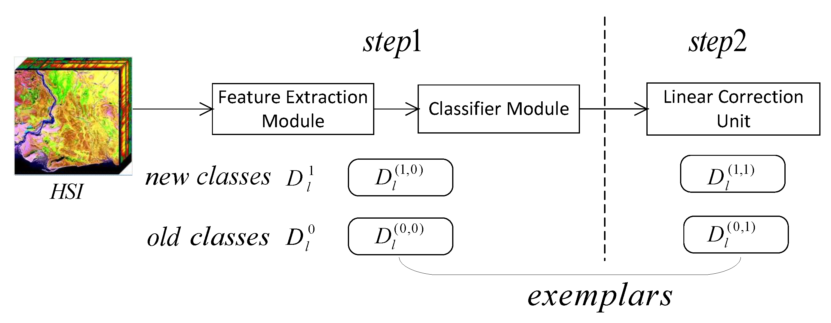
3. Methods
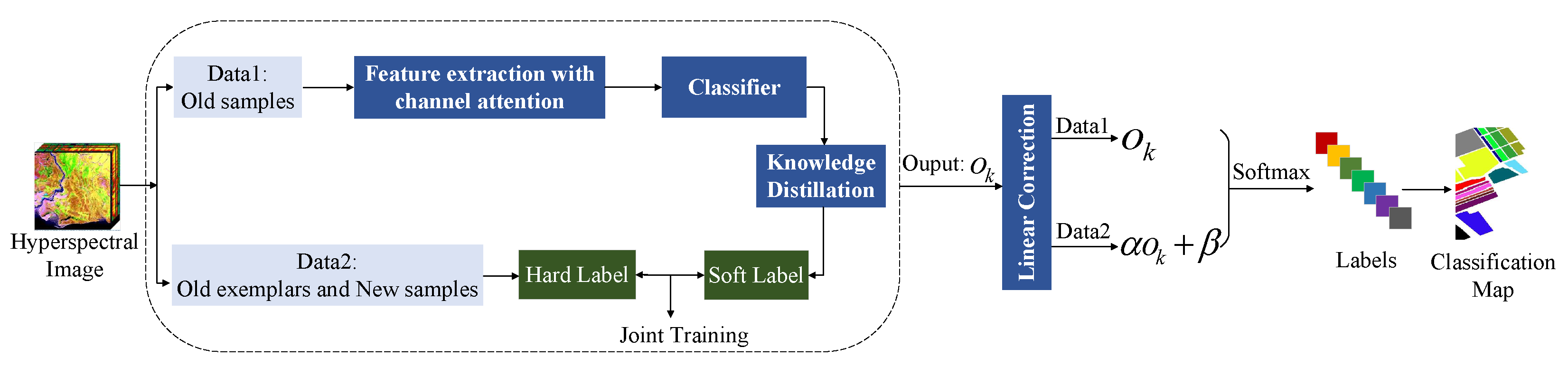
3.1. Framework
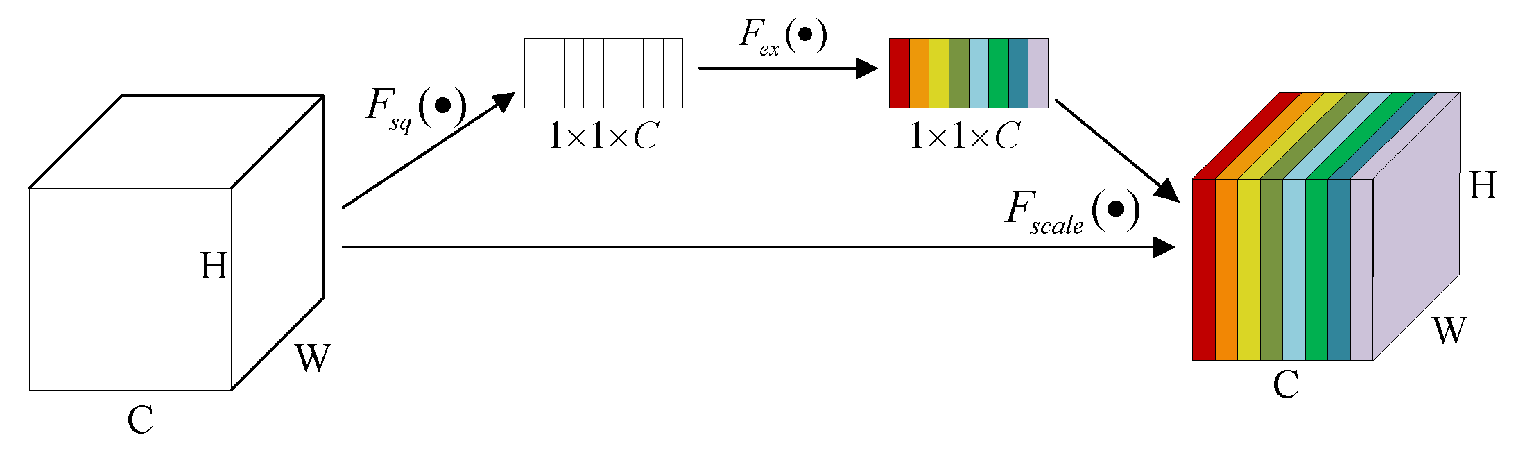
3.2. Channel Attention
3.3. Exemplars Management
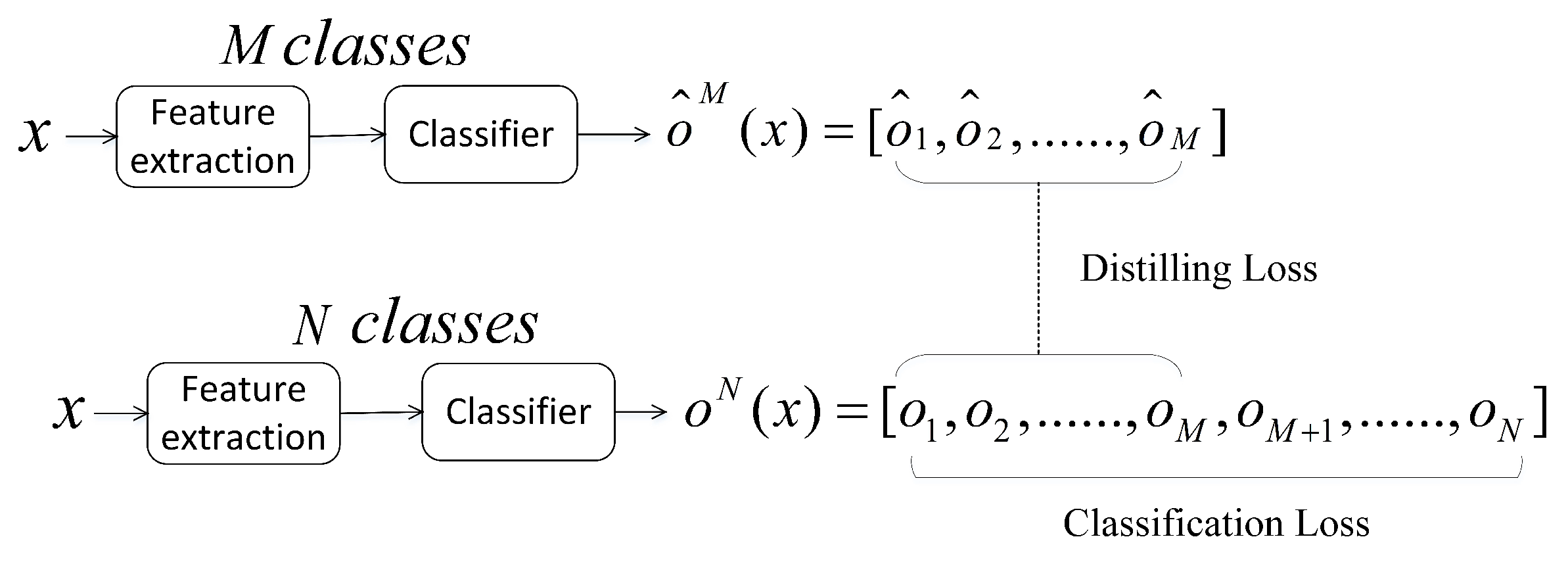
3.4. Knowledge Distillation
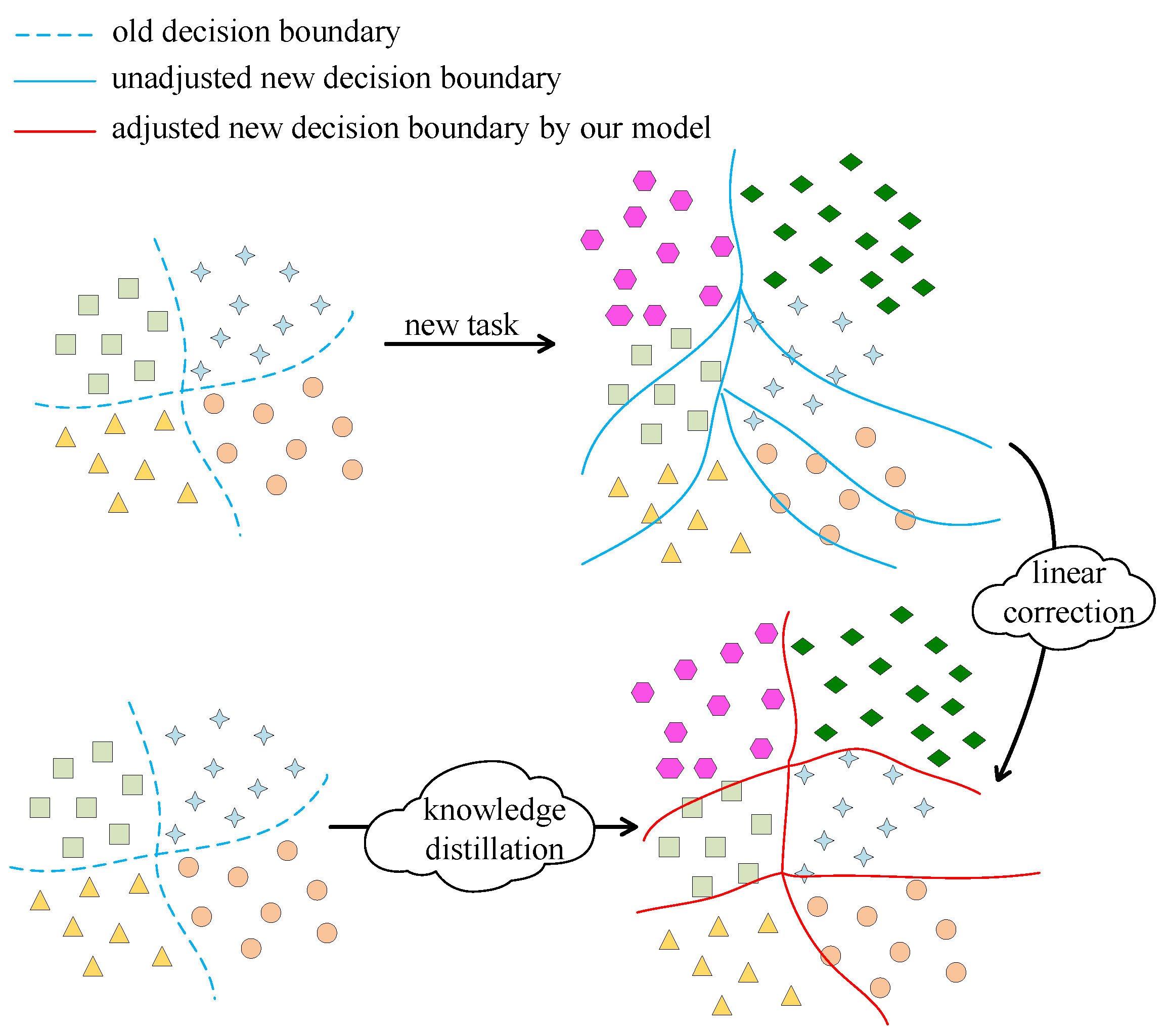
3.5. Linear Correction
| Algorithm 1 Class-Incremental Learning for HSI |
Input: ∈ // HSI data set L // learning phase P // the total number of old exemplars Output: OA, AA, // classification results of each phase |
4. Results
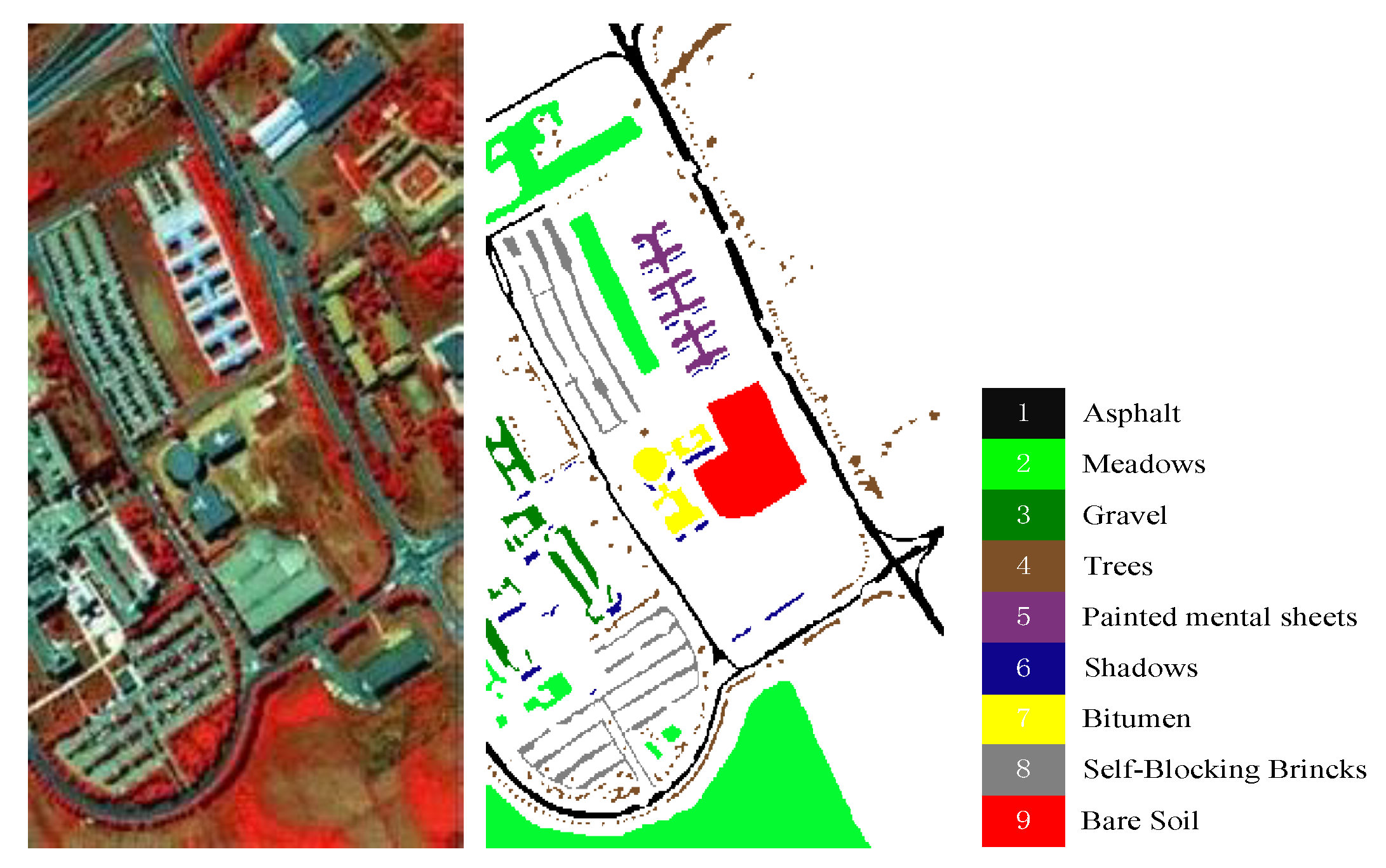
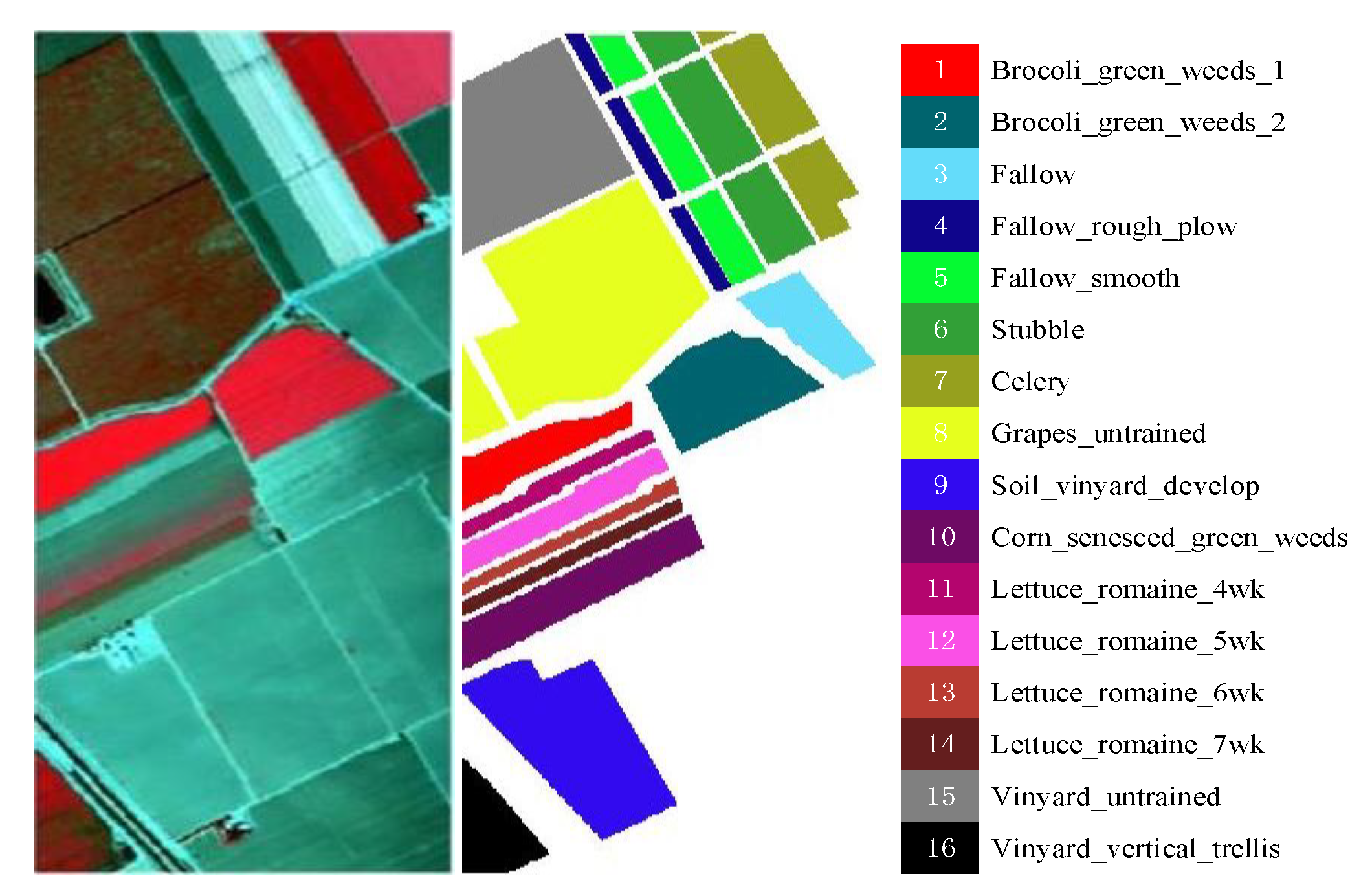
4.1. Data Description
4.2. Experimental Setup
4.3. Experimental Results
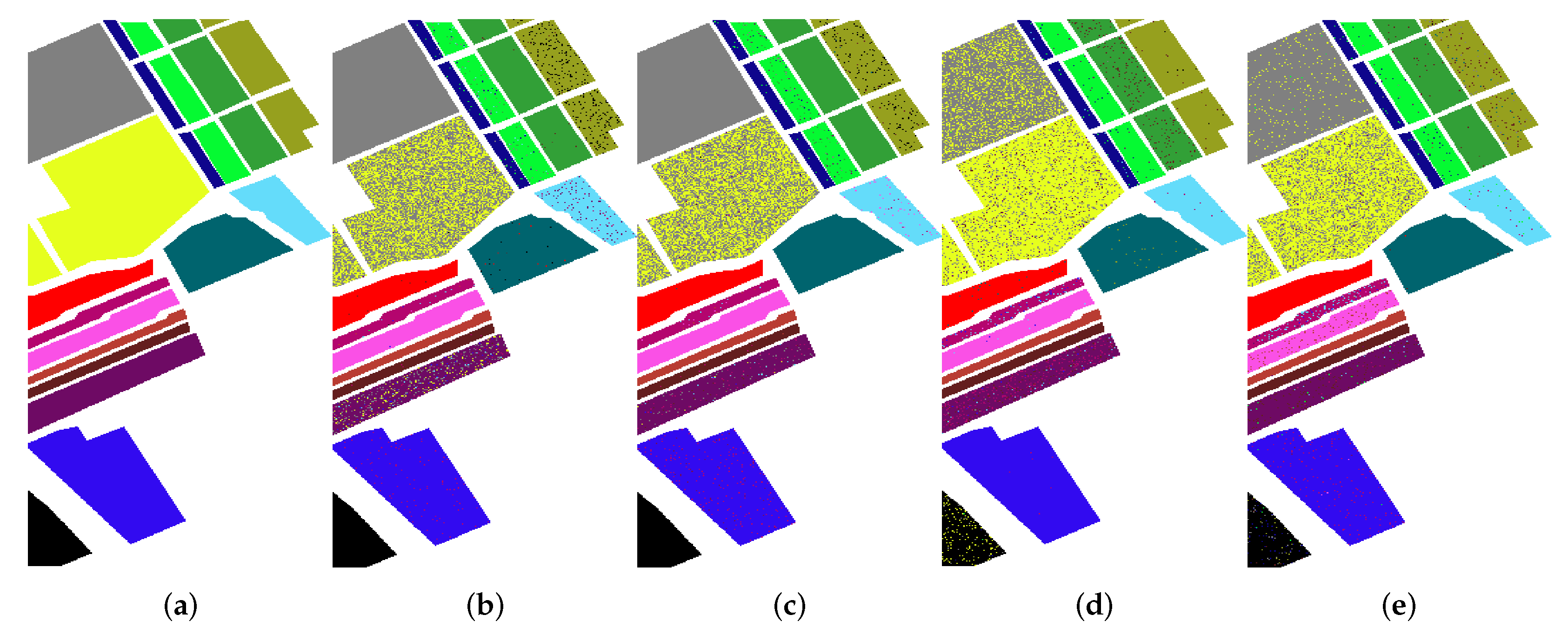
4.3.1. Ablation Experiments
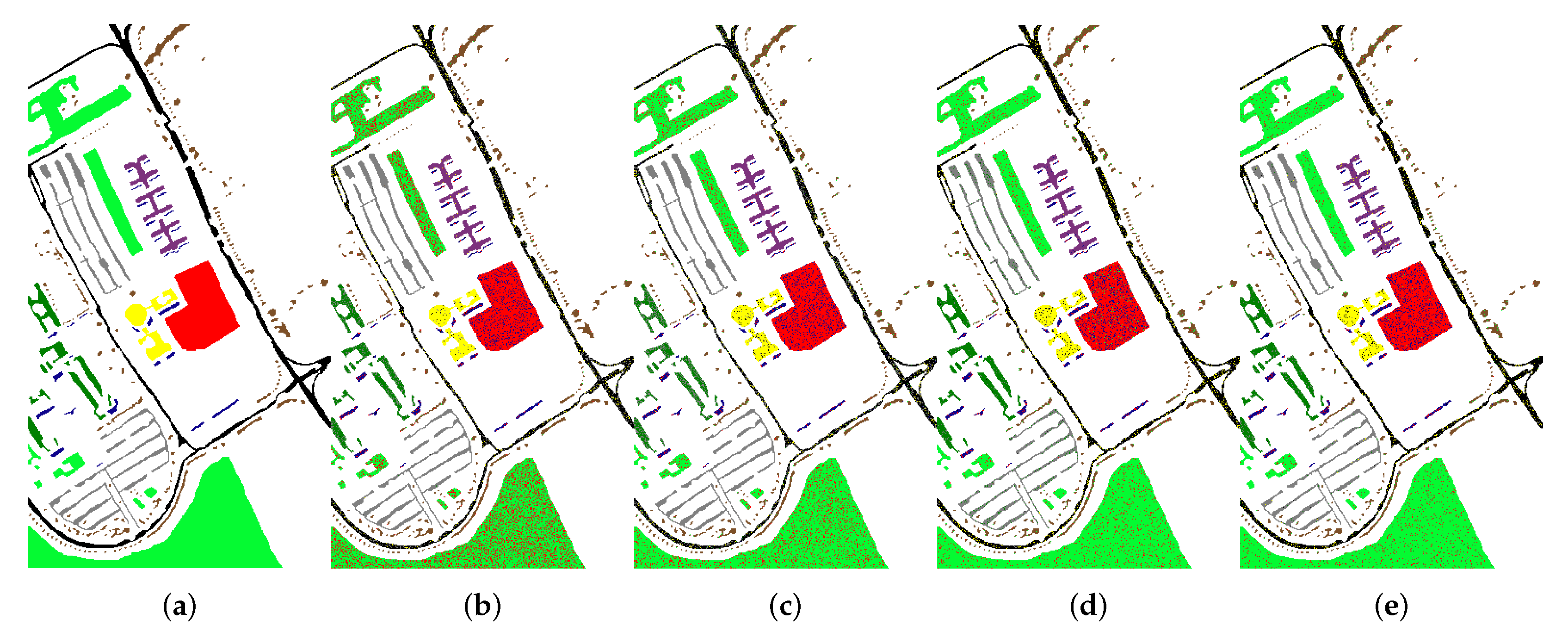
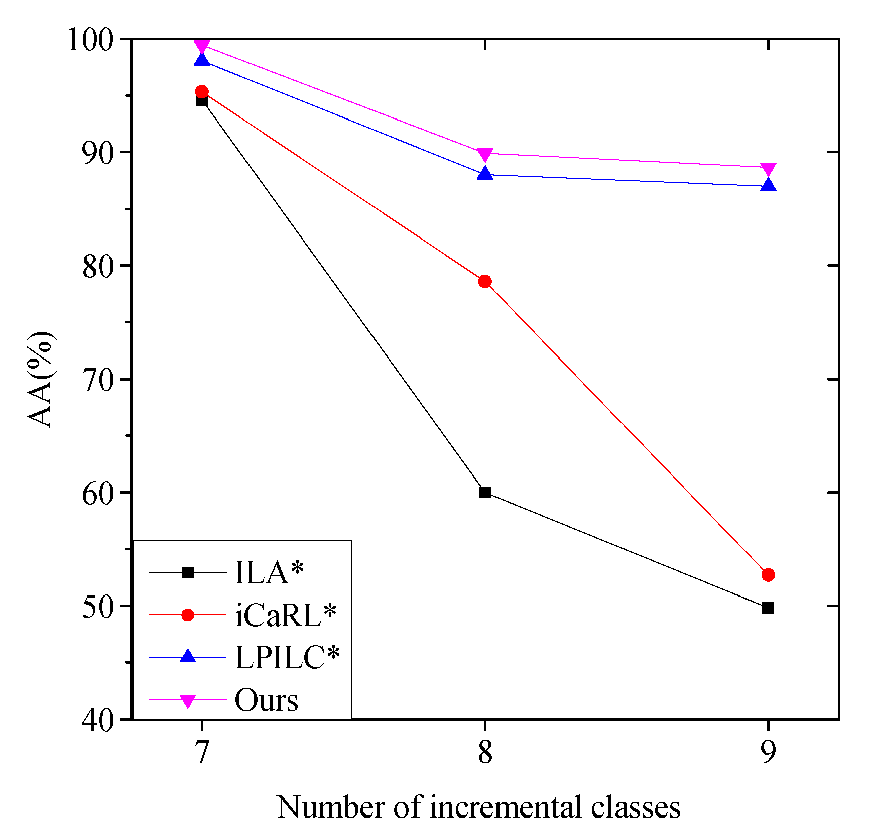
4.3.2. Comparison
5. Discussion
5.1. Parameters Analysis
5.1.1. Network Parameters
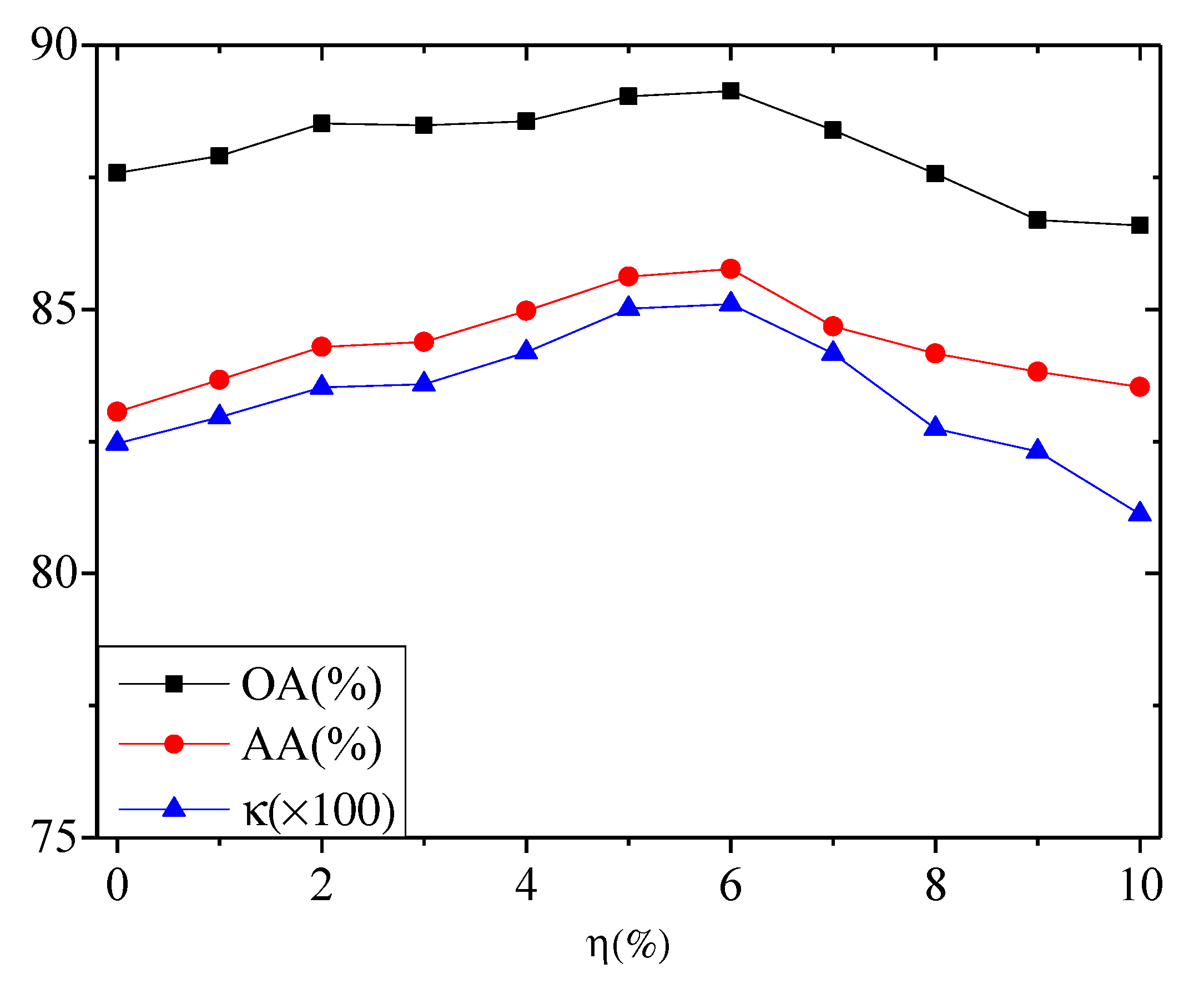
5.1.2. Hyperparameter
5.1.3. Sample Parameters
5.2. Memory Budget and Running Time
6. Conclusions
Author Contributions
Funding
Data Availability Statement
Acknowledgments
Conflicts of Interest
References
- Li, Z.; Huang, L.; He, J. A Multiscale Deep Middle-Level Feature Fusion Network for Hyperspectral Classification. Remote Sens. 2019, 11, 695. [Google Scholar] [CrossRef] [Green Version]
- Hsieh, T.H.; Kiang, J.F. Comparison of CNN Algorithms on Hyperspectral Image Classification in Agricultural Lands. Sensors 2020, 20, 1734. [Google Scholar] [CrossRef] [PubMed] [Green Version]
- Masoud, M.; Bahram, S.; Mohammad, R.; Fariba, M.; Yun, Z. Very Deep Convolutional Neural Networks for Complex Land Cover Mapping Using Multispectral Remote Sensing Imagery. Remote Sens. 2018, 10, 1119. [Google Scholar]
- Zhao, C.; Wang, Y.; Qi, B.; Wang, J. Global and Local Real-Time Anomaly Detectors for Hyperspectral Remote Sensing Imagery. Remote Sens. 2015, 7, 3966–3985. [Google Scholar] [CrossRef] [Green Version]
- Zhang, X.; Sun, Y.; Jiang, K.; Li, C.; Jiao, L.; Zhou, H. Spatial Sequential Recurrent Neural Network for Hyperspectral Image Classification. IEEE J. Sel. Top. Appl. Earth Observ. Remote Sens. 2018, 11, 4141–4155. [Google Scholar] [CrossRef] [Green Version]
- Liu, S.; Shi, Q.; Zhang, L. Few-Shot Hyperspectral Image Classification With Unknown Classes Using Multitask Deep Learning. IEEE Trans. Geosci. Remote Sens. 2020, 59, 5085–5102. [Google Scholar] [CrossRef]
- Melgani, F.; Bruzzone, L. Classification of Hyperspectral Remote Sensing Images with Support Vector Machines. IEEE Trans. Geosci. Remote Sens. 2004, 42, 1778–1790. [Google Scholar] [CrossRef] [Green Version]
- Plaza, J.; Plaza, A.J.; Barra, C. Multi-Channel Morphological Profiles for Classification of Hyperspectral Images Using Support Vector Machines. Sensors 2009, 9, 196–218. [Google Scholar] [CrossRef] [Green Version]
- Ma, W.; Gong, C.; Hu, Y.; Meng, P.; Xu, F.; Zhang, L.; Yang, J. The Hughes Phenomenon in Hyperspectral Classification Based on the Ground Spectrum of Grasslands in the Region Around Qinghai Lake. In International Symposium on Photoelectronic Detection and Imaging 2013: Imaging Spectrometer Technologies and Applications; International Society for Optics and Photonics: Washington, DC, USA, 2013; p. 89101G. [Google Scholar]
- Martinez-UsoMartinez-Uso, A.; Pla, F.; Sotoca, J.M.; Garcia-Sevilla, P. Clustering-Based Hyperspectral Band Selection Using Information Measures. IEEE Trans. Geosci. Remote Sens. 2007, 45, 4158–4171. [Google Scholar] [CrossRef]
- Licciardi, G.; Marpu, P.R.; Chanussot, J.; Benediktsson, J.A. Linear Versus Nonlinear PCA for the Classification of Hyperspectral Data Based on the Extended Morphological Profiles. IEEE Geosci. Remote Sens. Lett. 2012, 9, 447–451. [Google Scholar] [CrossRef] [Green Version]
- Li, H.; Xiao, G.; Xia, T.; Tang, Y.Y.; Li, L. Hyperspectral Image Classification Using Functional Data Analysis. IEEE Trans. Cybern. 2014, 44, 1544–1555. [Google Scholar] [PubMed]
- Bandos, T.V.; Bruzzone, L.; Camps-Valls, G. Classification of Hyperspectral Images With Regularized Linear Discriminant Analysis. IEEE Trans. Geosci. Remote Sens. 2009, 47, 862–873. [Google Scholar] [CrossRef]
- Fauvel, M.; Benediktsson, J.A.; Chanussot, J.; Sveinsson, J.R. Spectral and Spatial Classification of Hyperspectral Data Using SVMs and Morphological Profiles. IEEE Trans. Geosci. Remote Sens. 2008, 46, 3804–3814. [Google Scholar] [CrossRef] [Green Version]
- Patra, S.; Bhardwaj, K.; Bruzzone, L. A Spectral-Spatial Multicriteria Active Learning Technique for Hyperspectral Image Classification. IEEE J. Sel. Top. Appl. Earth Observ. Remote Sens. 2017, 10, 5213–5227. [Google Scholar] [CrossRef]
- Chen, Y.; Lin, Z.; Zhao, X.; Wang, G.; Gu, Y. Deep Learning-Based Classification of Hyperspectral Data. IEEE J. Sel. Top. Appl. Earth Observ. Remote Sens. 2014, 7, 2094–2107. [Google Scholar] [CrossRef]
- Cui, B.; Cui, J.; Hao, S.; Guo, N.; Lu, Y. Spectral-spatial hyperspectral image classification based on superpixel and multi-classifier fusion. Int. J. Remote. Sens. 2020, 41, 6157–6182. [Google Scholar] [CrossRef]
- Sk, A.; Kk, B.; Aa, C. A New CNN Training Approach with Application to Hyperspectral Image Classification. Digit. Signal Prog. 2021, 113, 103016. [Google Scholar]
- Li, Z.; Cui, X.; Wang, L.; Zhang, H.; Zhang, Y. Spectral and Spatial Global Context Attention for Hyperspectral Image Classification. Remote Sens. 2021, 13, 771. [Google Scholar] [CrossRef]
- French, R.M. Catastrophic forgetting in connectionist networks. Trends Cognit. Sci. 1999, 3, 128–135. [Google Scholar] [CrossRef]
- Wu, Y.; Chen, Y.; Wang, L.; Ye, Y.; Liu, Z.; Guo, Y.; Fu, Y. Large Scale Incremental Learning. In Proceedings of the IEEE/CVF Conference on Computer Vision and Pattern Recognition, Long Beach, CA, USA, 15–20 June 2019; Volume 1, pp. 374–382. [Google Scholar]
- Li, S.; Zhu, X.; Bao, J. Hierarchical Multi-Scale Convolutional Neural Networks for Hyperspectral Image Classification. Sensors 2019, 19, 1714. [Google Scholar] [CrossRef] [Green Version]
- Li, C.; Yang, S.X.; Yang, Y.; Gao, H.; Zhao, J.; Qu, X.; Wang, Y.; Yao, D.; Gao, J. Hyperspectral Remote Sensing Image Classification Based on Maximum Overlap Pooling Convolutional Neural Network. Sensors 2018, 18, 3587. [Google Scholar] [CrossRef] [Green Version]
- Tun, N.L.; Gavrilov, A.; Tun, N.M.; Trieu, D.M.; Aung, H. Hyperspectral Remote Sensing Images Classification Using Fully Convolutional Neural Network. In Proceedings of the 2021 IEEE Conference of Russian Young Researchers in Electrical and Electronic Engineering (ElConRus), St. Petersburg, Russia, 26–29 January 2021; pp. 2166–2170. [Google Scholar]
- Chen, Y.; Zhu, K.; Zhu, L.; He, X.; Ghamisi, P.; Benediktsson, J.A. Automatic Design of Convolutional Neural Network for Hyperspectral Image Classification. IEEE Trans. Geosci. Remote Sens. 2019, 57, 7048–7066. [Google Scholar] [CrossRef]
- Zhang, J.; Wei, F.; Feng, F.; Wang, C.y. Spatial–Spectral Feature Refinement for Hyperspectral Image Classification Based on Attention-Dense 3D-2D-CNN. Sensors 2020, 20, 5191. [Google Scholar] [CrossRef] [PubMed]
- Zhang, X.; Wang, Y.; Zhang, N.; Xu, D.; Luo, H.; Chen, B.; Ben, G. Spectral–Spatial Fractal Residual Convolutional Neural Network With Data Balance Augmentation for Hyperspectral Classification. IEEE Trans. Geosci. Remote Sens. 2021, 59, 10473–10487. [Google Scholar] [CrossRef]
- Ma, X.; Wang, H.; Geng, J. Spectral-Spatial Classification of Hyperspectral Image Based on Deep Auto-Encoder. IEEE J. Sel. Top. Appl. Earth Observ. Remote Sens. 2016, 9, 4073–4085. [Google Scholar] [CrossRef]
- Zhou, S.; Xue, Z.; Du, P. Semisupervised Stacked Autoencoder With Cotraining for Hyperspectral Image Classification. IEEE Trans. Geosci. Remote Sens. 2019, 57, 3813–3826. [Google Scholar] [CrossRef]
- Tao, C.; Pan, H.; Li, Y.; Zou, Z. Unsupervised Spectral-Spatial Feature Learning With Stacked Sparse Autoencoder for Hyperspectral Imagery Classification. IEEE Geosci. Remote Sens. Lett. 2015, 12, 2438–2442. [Google Scholar]
- Jinling, Z.; Lei, H.; Yingying, D.; Linsheng, H.; Shizhuang, W. A combination method of stacked autoencoder and 3D deep residual network for hyperspectral image classification. Int. J. Appl. Earth Obs. Geoinform. 2021, 102, 102459. [Google Scholar]
- Chen, Y.; Zhao, X.; Jia, X. Spectral-Spatial Classification of Hyperspectral Data Based on Deep Belief Network. IEEE J. Sel. Top. Appl. Earth Observ. Remote Sens. 2015, 8, 2381–2392. [Google Scholar] [CrossRef]
- Zhong, P.; Gong, Z.; Li, S.; Schonlieb, C.B. Learning to Diversify Deep Belief Networks for Hyperspectral Image Classification. IEEE Trans. Geosci. Remote Sens. 2017, 55, 3516–3530. [Google Scholar] [CrossRef]
- Arsa, D.M.S.; Jati, G.; Mantau, A.J.; Wasito, I. Dimensionality Reduction Using Deep Belief Network in Big Data Case Study: Hyperspectral Image Classification. In Proceedings of the 2016 International Workshop on Big Data and Information Security (IWBIS), Jakarta, Indonesia, 18–19 October 2016; pp. 71–76. [Google Scholar]
- Mughees, A.; Tao, L. Multiple Deep-Belief-Network-Based Spectral-Spatial Classification of Hyperspectral Images. Tsinghua Sci. Tech. 2019, 24, 183–194. [Google Scholar] [CrossRef]
- Chen, C.; Ma, Y.; Ren, G. Hyperspectral Classification Using Deep Belief Networks Based on Conjugate Gradient Update and Pixel-Centric Spectral Block Features. IEEE J. Sel. Top. Appl. Earth Observ. Remote Sens. 2020, 13, 4060–4069. [Google Scholar] [CrossRef]
- Liu, Y.; Cao, G.; Sun, Q.; Siegel, M. Hyperspectral Classification via Deep Networks and Superpixel Segmentation. Int. J. Remote Sens. 2015, 36, 3459–3482. [Google Scholar] [CrossRef]
- Chen, X.; Li, M.; Yang, X. Stacked Denoise Autoencoder Based Feature Extraction and Classification for Hyperspectral Images. J. Sens. 2015, 2016, 1–10. [Google Scholar]
- Rahaf, A.; Francesca, B.; Mohamed, E.; Marcus, R.; Tinne, T. Memory Aware Synapses: Learning what (not) to forget. In Proceedings of the European Conference on Computer Vision (ECCV), Munich, Germany, 8–14 September 2018; pp. 139–154. [Google Scholar]
- Li, Z.; Hoiem, D. Learning Without Forgetting. IEEE Trans. Pattern Anal. Mach. Intell. 2018, 40, 2935–2947. [Google Scholar] [CrossRef] [Green Version]
- Rannen, A.; Aljundi, R.; Blaschko, M.B.; Tuytelaars, T. Encoder Based Lifelong Learning. In Proceedings of the IEEE International Conference on Computer Vision, Venice, Italy, 22–29 October 2017; pp. 1329–1337. [Google Scholar]
- Zhu, F.; Zhang, X.Y.; Wang, C.; Yin, F.; Liu, C.L. Prototype Augmentation and Self-Supervision for Incremental Learning. In Proceedings of the IEEE/CVF Conference on Computer Vision and Pattern Recognition, Nashville, TN, USA, 20–25 June 2021; pp. 5867–5876. [Google Scholar]
- Jaehong, Y.; Eunho, Y.; Jungtae, L.; Hwang, S.J. Lifelong Learning with Dynamically Expandable Networks. arXiv 2017, arXiv:1708.01547. [Google Scholar]
- Mallya, A.; Davis, D.; Lazebnik, S. Piggyback: Adapting a Single Network to Multiple Tasks by Learning to Mask Weights. In Proceedings of the European Conference on Computer Vision, Munich, Germany, 8–14 September 2018; pp. 72–88. [Google Scholar]
- Serra, J.; Suris, D.; Miron, M.; Karatzoglou, A. Overcoming Catastrophic Forgetting with Hard Attention to the Task. Int. Conf. Mach. Learn. 2018, 80, 4548–4557. [Google Scholar]
- Achituve, I.; Navon, A.; Yemini, Y.; Chechik, G.; Fetaya, E. GP-Tree: A Gaussian Process Classifier for Few-Shot Incremental Learning. arXiv 2021, arXiv:2102.07868v4. [Google Scholar]
- Chaudhry, A.; Marc’Aurelio, R.; Rohrbach, M.; Elhoseiny, M. Efficient Lifelong Learning with A-GEM. arXiv 2019, arXiv:1812.00420. [Google Scholar]
- Rebuffi, S.A.; Kolesnikov, A.; Sperl, G.; Lampert, C.H. iCaRL: Incremental Classifier and Representation Learning. In Proceedings of the IEEE conference on Computer Vision and Pattern Recognition, Honolulu, HI, USA, 21–26 July 2017; pp. 5533–5542. [Google Scholar]
- Liu, Y.; Schiele, B.; Sun, Q. Adaptive Aggregation Networks for Class-Incremental Learning. In Proceedings of the IEEE/CVF Conference on Computer Vision and Pattern Recognition, Nashville, TN, USA, 20–25 June 2021; pp. 2544–2553. [Google Scholar]
- Yan, S.; Zhou, J.; Xie, J.; Zhang, S.; He, X. An EM Framework for Online Incremental Learning of Semantic Segmentation. arXiv 2021, arXiv:2108.03613. [Google Scholar]
- Cermelli, F.; Mancini, M.; Rota Bulo, S.; Ricci, E.; Caputo, B. Modeling the Background for Incremental Learning in Semantic Segmentation. In Proceedings of the IEEE/CVF Conference on Computer Vision and Pattern Recognition, Seattle, WA, USA, 13–19 June 2020; pp. 9230–9239. [Google Scholar]
- Guanglei, Y.; Enrico, F.; Dan, X.; Paolo, R.; Mingli, D.; Hao, T.; Xavier, A.P.; Elisa, R. Continual Attentive Fusion for Incremental Learning in Semantic Segmentation. arXiv 2022, arXiv:2202.00432. [Google Scholar]
- Fabio, C.; Massimiliano, M.; Samuel, R.B.; Elisa, R.; Barbara, C. Modeling the Background for Incremental and Weakly-Supervised Semantic Segmentation. arXiv 2022, arXiv:2201.13338. [Google Scholar]
- Tasar, O.; Tarabalka, Y.; Alliez, P. Incremental Learning for Semantic Segmentation of Large-Scale Remote Sensing Data. IEEE J. Sel. Top. Appl. Earth Observ. Remote Sens. 2019, 12, 3524–3537. [Google Scholar] [CrossRef] [Green Version]
- Bai, J.; Yuan, A.; Xiao, Z.; Zhou, H.; Wang, D.; Jiang, H.; Jiao, L. Class Incremental Learning With Few-Shots Based on Linear Programming for Hyperspectral Image Classification. IEEE Trans. Cybern. 2020, 1–12. [Google Scholar] [CrossRef]
- Hu, J.; Shen, L.; Albanie, S.; Sun, G.; Wu, E. Squeeze-and-Excitation Networks. In Proceedings of the IEEE Conference on Computer Vision and Pattern Recognition, Long Beach, CA, USA, 15–19 June 2019; pp. 7132–7141. [Google Scholar]
- Hou, S.; Pan, X.; Loy, C.C.; Wang, Z.; Lin, D. Learning a Unified Classifier Incrementally via Rebalancing. In Proceedings of the IEEE/CVF Conference on Computer Vision and Pattern Recognition (CVPR), Long Beach, CA, USA, 15–20 June 2019; pp. 831–839. [Google Scholar]
- Mariela, A.; Eduardo, G.; Rendón, E. Implementation of incremental learning in artificial neural networks. In Proceedings of the 3rd Global Conference on Artificial Intelligence (GCAI), Miami, FL, USA, 18–22 October 2017; pp. 221–232. [Google Scholar]


| Model | LC | Attention | ||
|---|---|---|---|---|
| 1 | ✓ | |||
| 2 | ✓ | ✓ | ||
| 3 | ✓ | ✓ | ✓ | |
| Ours | ✓ | ✓ | ✓ | ✓ |
| Model | Meas. | PaviaU | Salinas | Houston | |||||||||
|---|---|---|---|---|---|---|---|---|---|---|---|---|---|
| 1–5 | 1–7 | 1–9 | 1–8 | 1–10 | 1–12 | 1–14 | 1–16 | 1–9 | 1–11 | 1–13 | 1–15 | ||
| 1 | OA(%) | 99.90 | 92.05 | 75.30 | 99.89 | 96.52 | 95.93 | 95.47 | 80.81 | 99.23 | 86.85 | 80.31 | 75.64 |
| AA(%) | 99.87 | 89.24 | 79.08 | 99.77 | 95.95 | 95.64 | 95.31 | 89.67 | 99.33 | 87.54 | 80.18 | 77.53 | |
| (×100) | 99.84 | 88.20 | 69.24 | 99.87 | 95.62 | 94.80 | 94.63 | 77.79 | 99.12 | 85.02 | 77.53 | 73.16 | |
| 2 | OA(%) | 99.91 | 93.63 | 80.34 | 99.90 | 97.13 | 96.28 | 96.34 | 82.01 | 99.22 | 88.94 | 82.65 | 79.02 |
| AA(%) | 98.89 | 90.46 | 81.80 | 99.50 | 96.40 | 95.95 | 96.37 | 91.26 | 99.31 | 89.41 | 82.37 | 80.33 | |
| (×100) | 99.83 | 91.59 | 77.02 | 99.84 | 96.38 | 96.25 | 95.73 | 80.86 | 99.14 | 88.29 | 81.05 | 77.37 | |
| 3 | OA(%) | 99.91 | 96.85 | 88.18 | 99.90 | 97.22 | 96.43 | 96.18 | 86.25 | 99.22 | 91.24 | 86.70 | 86.27 |
| AA(%) | 99.88 | 93.86 | 85.57 | 99.79 | 97.06 | 96.19 | 96.65 | 93.08 | 99.32 | 90.42 | 84.29 | 85.93 | |
| (×100) | 99.85 | 95.15 | 84.28 | 99.81 | 96.48 | 96.36 | 96.25 | 85.49 | 99.10 | 90.27 | 84.95 | 84.31 | |
| Ours | OA(%) | 99.91 | 97.29 | 89.13 | 99.92 | 98.04 | 96.50 | 96.31 | 87.24 | 99.23 | 91.63 | 87.50 | 87.12 |
| AA(%) | 99.87 | 94.79 | 85.76 | 99.82 | 97.37 | 96.18 | 96.49 | 93.31 | 99.31 | 90.51 | 84.90 | 86.54 | |
| (×100) | 99.84 | 95.81 | 85.10 | 99.90 | 96.90 | 96.41 | 96.52 | 86.53 | 99.13 | 90.60 | 85.29 | 85.40 | |
| Class | LPILC | Ours |
|---|---|---|
| Asphalt | 98.56 | 97.91 |
| Meadows | 99.68 | 98.98 |
| Gravel | 94.25 | 92.65 |
| Trees | 92.4 | 95.74 |
| Painted Metal Sheets | 98.62 | 99.65 |
| Bare Soil | 99.37 | 98.10 |
| Bitumen | 93.96 | 92.42 |
| Self-Blocking Bricks | 95.04 | 86.57 |
| Shadows (new class) | 97.52 | 97.24 |
| Original OA(%) | 98.03 | 98.90 |
| New OA(%) | 97.52 | 97.24 |
| OA(%) | 98.02 | 96.59 |
| AA(%) | 96.60 | 95.47 |
| (×100) | 97.38 | 95.33 |
| Baseline | Parameter | Kernel Size | Measurement | Classes of PaviaU | ||
|---|---|---|---|---|---|---|
| 1–5 | 1–7 | 1–9 | ||||
| ResNet 6 | 2.41 M | 13 × 13 | OA(%) | 99.91 | 97.29 | 89.13 |
| AA(%) | 99.87 | 94.79 | 85.76 | |||
| (×100) | 99.84 | 95.81 | 85.10 | |||
| ResNet 8 | 5.96 M | 13 × 13 | OA(%) | 99.90 | 96.96 | 89.74 |
| AA(%) | 99.88 | 94.16 | 84.89 | |||
| (×100) | 99.82 | 94.76 | 85.13 | |||
| ResNet 6 | 2.41 M | 11 × 11 | OA(%) | 99.88 | 96.13 | 87.89 |
| AA(%) | 99.85 | 94.01 | 84.06 | |||
| (×100) | 99.81 | 94.38 | 83.92 | |||
| ResNet 6 | 2.41 M | 15 × 15 | OA(%) | 99.87 | 96.27 | 87.96 |
| AA(%) | 99.86 | 94.15 | 84.28 | |||
| (×100) | 99.80 | 94.40 | 84.57 | |||
| Split | Measurement | Classes of PaviaU | ||
|---|---|---|---|---|
| 1–5 | 1–7 | 1–9 | ||
| 9:1 | OA(%) | 99.90 | 96.87 | 88.32 |
| AA(%) | 99.87 | 94.05 | 84.88 | |
| (×100) | 99.83 | 95.84 | 83.96 | |
| 8:2 | OA(%) | 99.91 | 97.29 | 89.13 |
| AA(%) | 99.87 | 94.79 | 85.76 | |
| (×100) | 99.84 | 95.81 | 85.10 | |
| 7:3 | OA(%) | 99.90 | 97.04 | 88.87 |
| AA(%) | 99.88 | 94.27 | 84.82 | |
| (×100) | 99.83 | 95.43 | 83.75 | |
| 6:4 | OA(%) | 99.91 | 95.28 | 82.41 |
| AA(%) | 99.87 | 90.92 | 80.64 | |
| (×100) | 99.83 | 92.49 | 76.31 | |
| Phase | Method | Time | Data Memory |
|---|---|---|---|
| 0th | original | 1.28 min | 2.50 M |
| Ours | 1.28 min | 2.50 M | |
| 2nd | original | 1.47 min | 2.86 M |
| Ours | 0.86 min | 0.44 M | |
| 1st | original | 1.78 min | 3.36 M |
| Ours | 0.87 min | 0.58 M |
Publisher’s Note: MDPI stays neutral with regard to jurisdictional claims in published maps and institutional affiliations. |
© 2022 by the authors. Licensee MDPI, Basel, Switzerland. This article is an open access article distributed under the terms and conditions of the Creative Commons Attribution (CC BY) license (https://creativecommons.org/licenses/by/4.0/).
Share and Cite
Xu, M.; Zhao, Y.; Liang, Y.; Ma, X. Hyperspectral Image Classification Based on Class-Incremental Learning with Knowledge Distillation. Remote Sens. 2022, 14, 2556. https://doi.org/10.3390/rs14112556
Xu M, Zhao Y, Liang Y, Ma X. Hyperspectral Image Classification Based on Class-Incremental Learning with Knowledge Distillation. Remote Sensing. 2022; 14(11):2556. https://doi.org/10.3390/rs14112556
Chicago/Turabian StyleXu, Meng, Yuanyuan Zhao, Yajun Liang, and Xiaorui Ma. 2022. "Hyperspectral Image Classification Based on Class-Incremental Learning with Knowledge Distillation" Remote Sensing 14, no. 11: 2556. https://doi.org/10.3390/rs14112556
APA StyleXu, M., Zhao, Y., Liang, Y., & Ma, X. (2022). Hyperspectral Image Classification Based on Class-Incremental Learning with Knowledge Distillation. Remote Sensing, 14(11), 2556. https://doi.org/10.3390/rs14112556