Forest Fire Monitoring and Positioning Improvement at Subpixel Level: Application to Himawari-8 Fire Products

Abstract

Forest fires are among the biggest threats to forest ecosystems and forest resources, and can lead to ecological disasters and social crises. Therefore, it is imperative to detect and extinguish forest fires in time to reduce their negative impacts. Satellite remote sensing, especially meteorological satellites, has been a useful tool for forest-fire detection and monitoring because of its high temporal resolution over large areas. Researchers monitor forest fires directly at pixel level, which usually presents a mixture of forest and fire, but the low spatial resolution of such mixed pixels cannot accurately locate the exact position of the fire, and the optimal time window for fire suppression can thus be missed. In order to improve the positioning accuracy of the origin of forest fire (OriFF), we proposed a mixed-pixel unmixing integrated with pixel-swapping algorithm (MPU-PSA) model to monitor the OriFFs in time. We then applied the model to the Japanese Himawari-8 Geostationary Meteorological Satellite data to obtain forest-fire products at subpixel level. In this study, the ground truth data were provided by the Department of Emergency Management of Hunan Province, China. To validate the positioning accuracy of MPU-PSA for OriFFs, we applied the model to the Himawari-8 satellite data and then compared the derived fire results with fifteen reference forest-fire events that occurred in Hunan Province, China. The results show that the extracted forest-fire locations using the proposed method, referred to as forest fire locations at subpixel (FFLS) level, were far closer to the actual OriFFs than those from the modified Himawari-8 Wild Fire Product (M-HWFP). This improvement will help to reduce false fire claims in the Himawari-8 Wild Fire Product (HWFP). We conducted a comparative study of M-HWFP and FFLS products using three accuracy-evaluation indexes, i.e., Euclidean distance, RMSE, and MAE. The mean distances between M-HWFP fire locations and OriFFs and between FFLS fire locations and OriFFs were 3362.21 m and 1294.00 m, respectively. The mean RMSEs of the M-HWFP and FFLS products are 1225.52 m and 474.93 m, respectively. The mean MAEs of the M-HWFP and FFLS products are 992.12 m and 387.13 m, respectively. We concluded that the newly proposed MPU-PSA method can extract forest-fire locations at subpixel level, providing higher positioning accuracy of forest fires for their suppression.

1. Introduction

Forest fires, when not suppressed in time, can spread over large areas and sometimes may last for years or decades. There were a total of 116,171 active forest-fire events in China from 2001 to 2015 [1]. Forest-associated biomass burning could be, in part, responsible for the increase in greenhouse gases (GHG) in the atmosphere [2,3]. Forest fires are among the biggest threats to plant ecological systems and resources [1,4], and can cause ecological disasters and social crises. For instance, in Liangshan Yi Autonomous Prefecture, Sichuan Province, China, serious forest fires occurred three times during 2019–2021 causing 49 casualties [5,6,7], and the 2019–2020 Australia megafires lasted for five months from September 2019 to February 2020, killing or displacing nearly 3 billion animals [8].

A series of precautions should be taken to mitigate adverse fire impacts and reduce the likelihood of forest fires [9]. Effective forest-fire detection and monitoring has always been a strong focus of research [10,11,12,13,14]. Meteorological satellites can acquire data continuously over large areas and in high temporal resolution. Thus, they have been widely used for forest-fire detection and monitoring [13,15,16,17,18]. Over the past decades, based on the data from geostationary orbit (GEO) satellites or polar-orbiting satellites, researchers have proposed many forest-fire detection and monitoring algorithms. These can be divided into five categories [19]: (1) bi-spectral methods, such as that of Dozier [20], measuring the surface radiant temperature of subpixel spatial resolution; (2) modified bi-spectral methods, such as multiple endmember spectral mixture analysis (MESMA) [21], bi-spectral infrared detection (BIRD) [22], and the Giglio and Schroeder [23] method; (3) threshold methods, such as multi-channel threshold algorithms [24]; (4) spatial contextual methods, such as MODIS Collection 6 active fire algorithms [25]; and (5) multi-temporal fire detection methods, such as robust satellite techniques for FIRES detection and monitoring (RST-FIRES) algorithm [14]. However, due to the low spatial resolution of the satellites, researchers conduct forest-fire monitoring research directly at pixel scale, which can lead to significant fire-positioning error when the pixel shows a mixture of forest and fire [16,26,27,28,29,30]. Atkinson [31,32] first proposed the subpixel concept to find specific spatial distribution information in a mixed pixel. Forest-fire spatial location must be specified in a mixed pixel at the subpixel level.

For satellite data of low spatial resolution, mixed pixels are a common phenomenon [33,34,35]. They can be an obstacle in remote sensing applications in forest-fire detection, causing the estimated location of a forest fire to vary widely from the actual position, depending on spatial resolution. To overcome this obstacle, researchers proposed the traditional exponential model, which is often found to produce inconsistent results, since a mixed pixel includes both objective and non-objective materials [36]. A series of unmixing methods have been proposed, such as maximum-margin criterion and derivative weights (MDWSU) [37], minimum-volume transform (MVT) [38], vertex component analysis (VCA) [39], simplex growing algorithm (SGA) [40], minimum-volume-constrained nonnegative matrix factorization (MVC-NMF) [41], successive projection algorithm (SPA) [42], etc. He et al. [36] showed that spectral unmixing methods have advantages over the traditional exponential model due to their ability to decompose the mixed pixel into several fractional abundances. Shao and Lan [37] used the MDWSU technique to obtain more accurate endmembers and abundance estimates. Nascimento and Dias [39] performed a series of experiments using simulated and real data, and found that the VCA algorithm performs better than the pixel purity index (PPI) method, and better than or similar to the N-FINDR algorithms [43]. Miao and Qi [41] proposed the MVC-NMF method to extract unsupervised endmembers from highly mixed image data. Zhang et al. [42] proposed SPA, which can provide a general guideline to constrain the total number of endmembers.

However, spectral unmixing methods only solve the problem of endmember types and abundances, without determining endmember location in a mixed pixel. To solve this problem, Atkinson [31,32] proposed the subpixel concept for identifying precise spatial locations of endmembers in a mixed pixel based on unmixing analysis results [44]. On the basis of Atkinson’s study, many algorithms have been developed [45], such as spatial attraction model (SAM), double-calculated spatial attraction model (DSAM) [34], subpixel learning algorithms [46], subpixel edge-detection method [47], and so on. These subpixel techniques have found many applications [48,49,50,51]. For instance, the random forests and Spatial Attraction Model (RFSAM) was applied to remote sensing images to improve the accuracy of subpixel mapping of wetland flooding [52]. Li et al. [53] proposed the spatiotemporal subpixel land cover mapping (STSPM) method, demonstrating that it can predict land cover maps accurately. Ling et al. [54] proposed a new approach aimed at efficiently and accurately monitoring reservoir surface water area variations using daily moderate resolution imaging spectroradiometer (MODIS) images to explore subpixel scale information. Deng and Zhu [55] proposed the continuous subpixel monitoring (CSM) method and successfully applied it to mapping urban impervious surface area (ISA %) at subpixel scale and characterizing its dynamics in Broome County, New York.

However, there are very few applications of these subpixel algorithms to forest-fire location detection and fire monitoring [21]. In order to rapidly detect and monitor forest-fire locations to reduce damage and save lives and properties, ascertaining the exact locations of the origins of fires is important in order to gain quick access for firefighters. Subpixel algorithms can help locate fires with subpixel accuracy. However, current forest-fire monitoring methods using remote sensing data can locate forest fires only at pixel-size level. Location accuracy can be improved with subpixel-level detection.

The objective of this study is to develop a new algorithm to improve the detection of fire locations at subpixel level. To this end, we proposed a mixed pixel unmixing integrated with pixel-swapping algorithm (MPU-PSA) model, in which spectral unmixing analysis is performed using the Newton’s Method, then the unmixing analysis results are processed with the pixel-swapping algorithm to obtain OriFFs of forest fires. We then applied the new algorithm to the Himawari-8 L1 gridded data (HLGD) and Himawari-8 Wild Fire Product (HWFP), taking advantage of the high temporal resolution of the Himawari-8 satellite data to achieve more accurate forest-fire locations. The forest-fire information provided by the Department of Emergency Management of Hunan Province, China, was used as ground truth reference data. The result showed that the algorithm improved the location accuracy of the origin of forest fire (OriFF), saving time for forest-fire extinguishment.

2. Materials and Methods

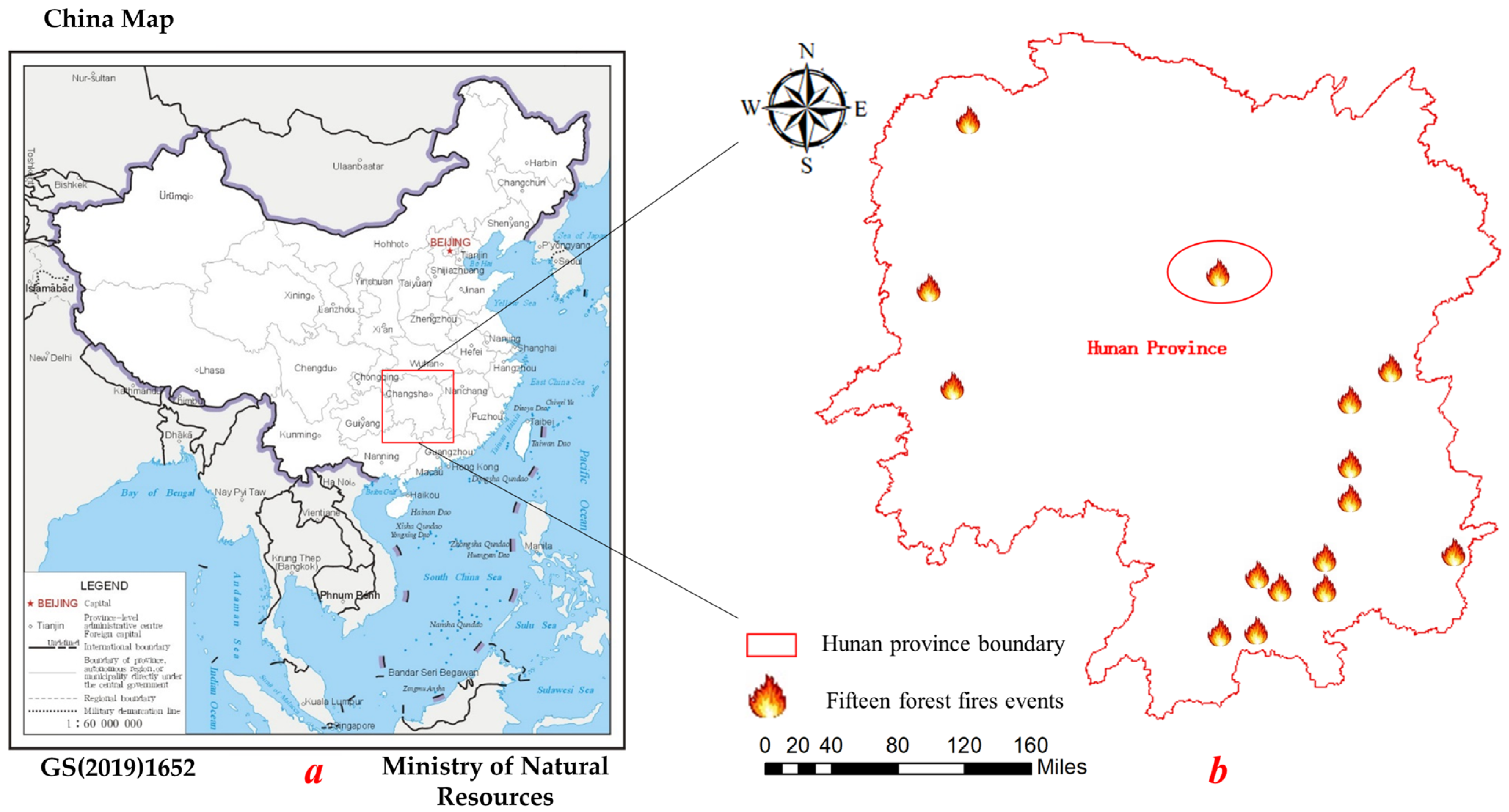
The present research used the following data: (a) satellite data, including Himawari-8, Sentinel 2, and Landsat 8 satellite data (Section 2.2); (b) ground truth data (Section 2.4). First, we ordered the Himawari-8 (https://www.eorc.jaxa.jp/ptree/, accessed on 10 December 2021) HLGD and HWFP data for the dates closest to the starting time of a forest fire. Then, band 7 and band 14 of the HLGD data were selected and fused to produce dataset B7_14 in Matlab R2016a (v 9.0, Mathworks, Natick, MA, USA). Wildfires detected in the HWFP data that did not match the ground truth forest-fire information were eliminated to generate the modified Himawari-8 Wild Fire Product (M-HWFP) dataset, but this remained at pixel level. Finally, the datasets B7_14 and M-HWFP were used as inputs to our proposed model to obtain the fire dataset forest-fire locations at subpixel (FFLS) level. Figure 1 shows the flowchart of data processing and analysis, which are explained in detail over the following sub-sections.

2.1. Study Area

Hunan Province is located in the middle Yangtze River, central China, within an area enclosed by 108°47′~114°15′ longitude and 24°38′~30°08′ latitude (Figure 2). Over a year, the temperature in Hunan Province typically varies from 7.78 °C to 33.33 °C. The rainiest month is June, with an average rainfall of 177.8 mm. The driest month is December, with an average rainfall of 35.56 mm. The relatively warm and humid weather results in lush vegetation and an evergreen landscape. Hunan province has a subtropical evergreen broad-leaved forest area with a forest coverage rate of 59.96%. Forest and wetland ecosystems are two major natural ecosystems. The ecological service function of the forest ecosystems in Hunan Province is worth 1.01 trillion Chinese Yuan. There are about 200 significant ecological zones around the world. Hunan province has two forest and wetland ecosystems (subtropical evergreen broad-leaved forest ecological zones in the Wuling Xuefeng Mountains and the Nanling Luoxiao Mountains), and they are known as the world’s most valuable ecological regions within their latitude zone. Due to the high forest coverage rate in Hunan Province, China, forest fires are significant potential hazards. Therefore, monitoring and rapidly suppressing forest fires is imperative for maintaining ecological integrity.

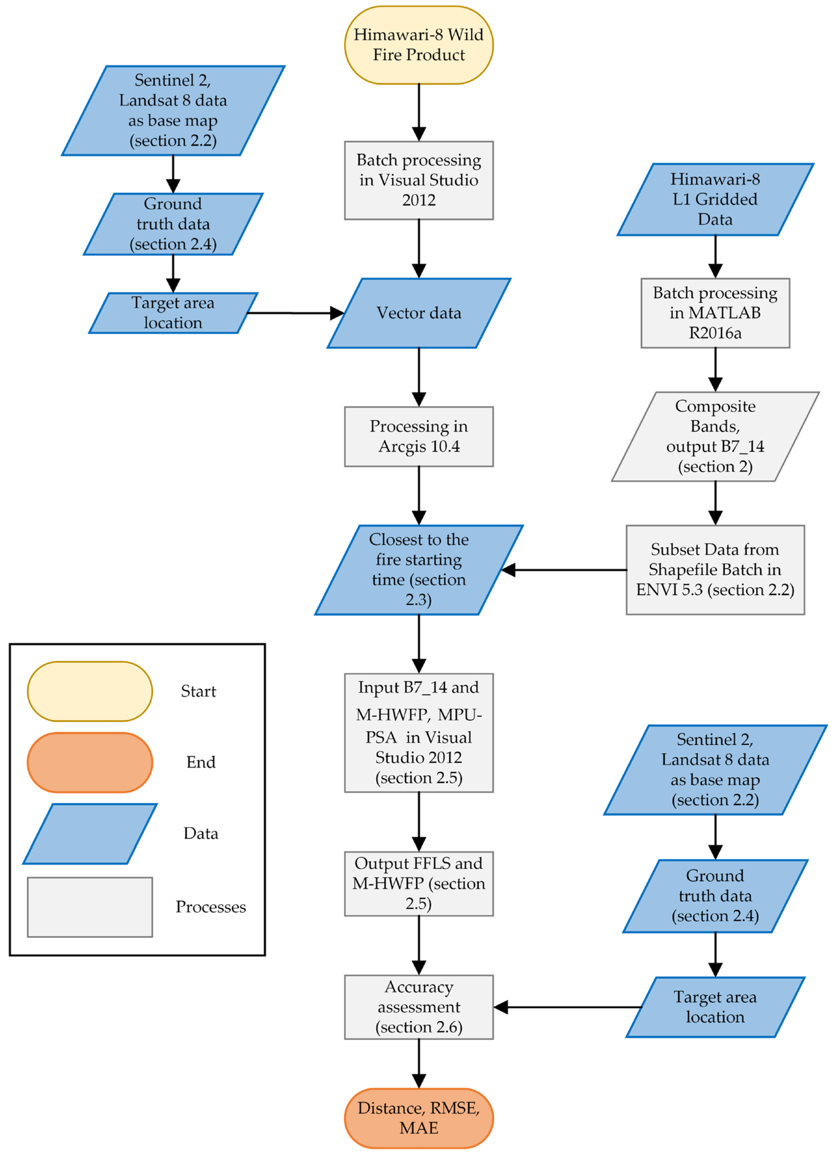
2.2. Satellite Data Processing

Himawari-8, Sentinel 2, and Landsat 8 satellite data were reprojected into a common Universal Transverse Mercator (UTM) projection with WGS84 as the datum so that all datasets could be overlaid within the same coordinate system. After each satellite dataset was clipped, the cloud cover was less than 10%. The Himawari-8 satellite data were used for detecting and monitoring the OriFF attribute at high temporal resolution (10 min). The Sentinel 2 and Landsat 8 images with higher spatial resolution were used as base maps to verify whether the hotspots detected in the Himawari-8 data were within the forest.

In this study, the HLGD data in Network Common Data Form (NetCDF) format and the HWFP data in comma-separated values (CSV) format were downloaded via File Transfer Protocol (FTP) in FileZilla Client 3.3.2 software. The Advanced Himawari Imager (AHI) carried by the Himawari-8 satellite scans the Pacific Ocean hemispheric region every 10 min, resulting in the production of 142 images over a specific scene per day [30,56]. The high temporal resolution of the Himawari-8 data makes it possible to semi-continuously monitor and detect forest fires, even though its spatial resolution is low. The JAXA Himawari Monitor User’s Guide is available on website https://www.eorc.jaxa.jp/ptree/userguide.html (accessed on 12 December 2021).

Table 1. Bands of Himawari-8 HLGD, Sentinel 2, and Landsat 8 imagery used in current study.

Satellite	Sensor	Band Number	Band Width (μm)	Spatial Resolution (m)
Himawari-8	AHI	7	3.74~3.96	2000
		14	11.10~11.30	2000
Sentinel 2	MSI	2	0.46~0.52	10
		3	0.54~0.58	10
		4	0.65~0.68	10
		8	0.79~0.90	10
Landsat 8	OLI	2	0.45~0.51	30
		3	0.53~0.59	30
		4	0.64~0.67	30
		5	0.85~0.88	30
		8	0.50~0.68	15

shows the characteristics of band 7 (3.85 μm) and band 14 (11.20 μm) selected for this study. These two bands are the most important bands used for forest-fire monitoring and detection [13,16,30]. This study acquired 2130 HLGD images and 2130 HWFP images for the fifteen forest-fire events used as reference fires. To reduce the influence of clouds, we filtered the clouds for each pixel when calculating the average background brightness temperature. Furthermore, to improve the running speed, we used the subset data from shapefile batch of ENVI 5.3 to clip HLGD.

The Sentinel 2 satellite data were downloaded from https://earthexplorer.usgs.gov/ (accessed on 15 December 2021) as Level 1C product. This product was orthorectified to top-of-atmosphere (TOA) reflectance. The Sentinel 2 satellite data were packaged into images according to the spatial resolution of 10 m (band 2, 3, 4, and 8), 20 m (bands 5, 6, 7, 8b, 11, and 12), and 60 m (bands 1, 9, and 10), respectively. The Sentinel 2 TOA reflectance data were processed to bottom-of-atmosphere (BOA) reflectance after radiometric calibration and atmospheric correction using Sen2cor (V2.8). Table 1 shows the characteristics of band 2 (Blue), band 3 (Green), band 4 (Red), and band 8 (NIR) selected for this study.

In this study, we used Landsat 8 OLI/TIRS C2 L1 data from https://earthexplorer.usgs.gov/ (accessed on 18 December 2021). The OLI/Landsat 8 multispectral and panchromatic data were processed to obtain the data-fusion result, using NNDiffuse Pan Sharpening in the ENVI 5.3 software. Table 1 shows the characteristics of band 2 (Blue), band 3 (Green), band 4 (Red), band 5 (NIR), and band 8 (Pan) of Landsat 8 selected for this study.

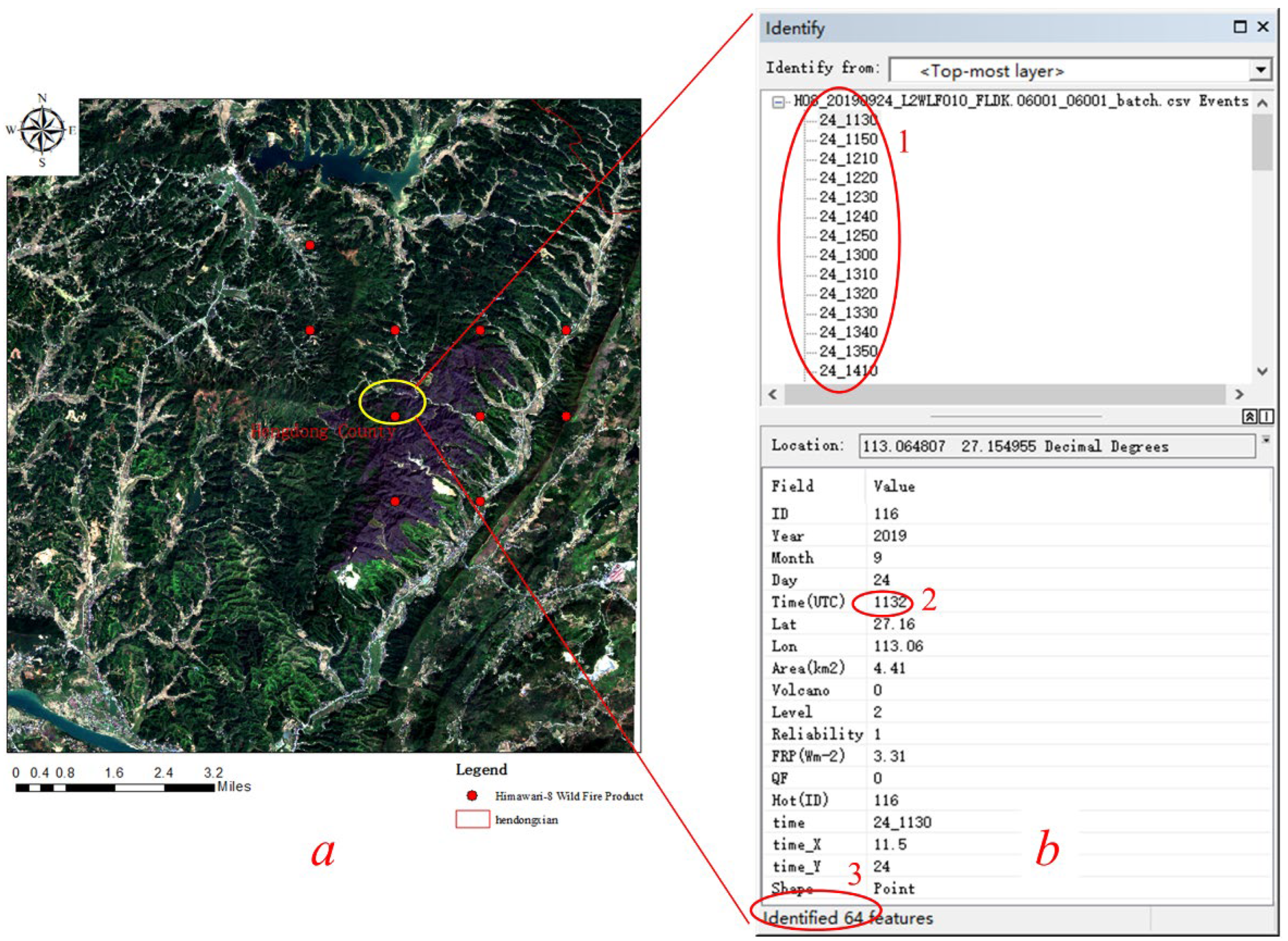
2.3. Input Data Preparation

Using Visual Studio 2012 software based on C# programming (https://github.com/HZXu1/MPU_PSA.git, accessed on 10 May 2022), we batch-processed the 142 HWFP daily images and extracted and saved hotspot information in a CSV file. Furthermore, all hotspot information of the 142 HWFP images, especially the earliest UTC time of every forest-fire event, was obtained using ArcGIS 10.4 software through the tabulated collected fire information (TCFI). For example, taking the first wildfire event (i.e., 1HeCo, which is the serial number of forest-fire event) (Figure 3), the red dot inside the yellow circle in the HWFP image gives the location of a hotspot in the IR images detected 64 times that day, as indicated in the third red circle (Figure 3b). False fires in the HWFP images were eliminated by comparing them to the TCFI data and burned area base map, and a Modified Himawari-8 Wild Fire Product (M-HWFP) was obtained. Combining the base map and TCFI data, we can see that the earliest monitoring time of the forest-fire event was 11:32 am (UTC time). Then, the M-HWFP data and the preprocessed HLGD data obtained at the timepoint closest to a fire’s starting time in a target area were used as input to the Visual Studio 2012 software based on C# programming.

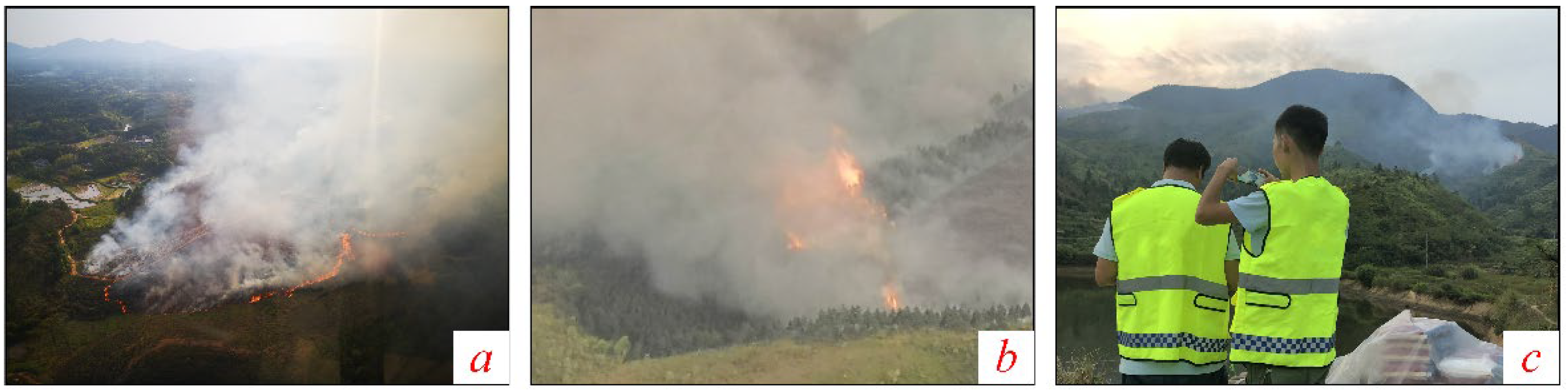
2.4. Ground Truth Data

Tabulated collected fire information (TCFI) as provided by the Department of Emergency Management of Hunan Province was used as ground truth data. Information about each fire event includes location, weather, starting and extinguishing times, damaged area, and cause. The Department of Emergency Management of Hunan Province confirms and reports forest-fire events when a forest fire occurs (Figure 4). Field measurements, including those pertaining to OriFF and damaged areas from a forest fire, were performed by well-trained personnel with global navigation satellite system survey equipment and unmanned aerial vehicles (UAV. The type of platform was Phantom 4 Pro V2.0, and the sensor was 1-inch CMOS with 20 million effective pixels. After the route was designed, the data were automatically collected and stored in the fuselage memory card). From the TCFI data between 2018 and 2021, the fifteen forest-fire events that resulted in the most environmental damage were selected as reference data.

2.5. The Proposed MPU-PSA Model

The proposed MPU-PSA model consists of two major procedures: (1) pixel-unmixing analysis using Newton’s method, and (2) derivation of forest-fire spatial distribution information using pixel-Swapping algorithm (PSA). We used the MPU-PSA method to improve determination of the spatial locations of forest fires at a subpixel scale. The M-HWFP and B7_14 datasets were processed using the MPU-PSA method to obtain the final result. Based on the Himawari-8 satellite data, each pixel was evenly divided into 5 × 5 subpixels. The spatial resolution of each subpixel was thus 400 m. The final result was forest-fire spatial distribution information in a mixed pixel.

2.5.1. Mixed Pixel-Unmixing (MPU) Analysis

The Planck function for emittance at wavelength λ of a blackbody at kinetic temperature T is shown in Equation (1):

$$M_{\lambda ,T}=\frac{2\pi h{\mathrm{c}}^2}{{\lambda }^5({\exp }^{h\mathrm{c}/kT\lambda }-1)}=\frac{{\mathrm{C}}_1}{{\lambda }^5({\exp }^{C_2/\lambda \cdot T}-1)}$$

(1)

The method for satellite identification of surface temperature fields at subpixel resolution was proposed by Dozier [20]. Assuming a mixed pixel is composed of active fire with high temperature in proportion P (where 0 ≤ P ≤ 1) and a background with normal temperature in the remaining proportion (1 − P), radiance of a mixed pixel can be expressed by the following Equation (2):

$$L_i=P\times L_{i,fire}+(1-P)\times L_{i,bg}=P\times \frac{{\mathrm{C}}_1}{\pi {\lambda }_{\mathrm{i}}{}^5({\exp }^{{C_2/{\lambda }_i\cdot T}_{i,fire}}-1)}+(1-P)\times \frac{{\mathrm{C}}_1}{\pi {\lambda }_i{}^5({\exp }^{{C_2/{\lambda }_i\cdot T}_{i,bg}}-1)}$$

(2)

where subscript i indicates the i-th band; $L_i$ is the radiance at i-th band (W·m⁻²·μm⁻¹·sr⁻¹); L_{i, fire} the target forest-fire radiance (W·m⁻²·μm⁻¹·sr⁻¹); L_{i, bg} the background (bg) radiance (W·m⁻²·μm⁻¹·sr⁻¹); C₁ and C₂ are the first (3.74 × 10⁻¹⁶ W·m²) and second (1.44 × 10⁻² m·K) Planck constants, respectively; λ_i is the wavelength (μm) of i-th band; and T_{i, fire} and T_i,bg are the temperature (K) of the target forest fire and the background, respectively. We chose band 7 and band 14 in this study, and the radiances of a mixed pixel for band 7 and band 14 were given as below according to Equation (2).

$$\{\begin{array}{c}{L}_7=P\times L_{7,fire}+(1-P)\times L_{7,bg}\\ L_{14}=P\times L_{14,fire}+(1-P)\times L_{14,bg}\end{array}$$

(3)

where

$$L_{7,fire}=\frac{{\mathrm{C}}_1}{\pi {\lambda }_7{}^5({\exp }^{{C_2/{\lambda }_7\cdot T}_{7,fire}}-1)},L_{7,bg}=\frac{{\mathrm{C}}_1}{\pi {\lambda }_7{}^5({\exp }^{{C_2/{\lambda }_7\cdot T}_{7,bg}}-1)},L_{14,fire}=\frac{{\mathrm{C}}_1}{\pi {\lambda }_{14}{}^5({\exp }^{{C_2/{\lambda }_{14}\cdot T}_{14,fire}}-1)},\mathrm{and}{L}_{14,bg}=\frac{{\mathrm{C}}_1}{\pi {\lambda }_{14}{}^5({\exp }^{{C_2/{\lambda }_{14}\cdot T}_{14,bg}}-1)}$$

Rearranging Equation (3), we obtained Equation (4), where we introduced two objective functions, $\mathrm{F}(P,T_{7fire})$ and $\mathrm{G}(P,T_{14fire})$:

$$\{\begin{array}{c}\mathrm{F}(P,T_{7,fire})=-L_7+P\times \frac{{\mathrm{C}}_1}{\pi {\lambda }_7{}^5({\exp }^{{C_2/{\lambda }_7\cdot T}_{7fire}}-1)}+(1-P)\times \frac{{\mathrm{C}}_1}{\pi {\lambda }_7{}^5({\exp }^{{C_2/{\lambda }_7\cdot T}_{7bg}}-1)}=0\\ \mathrm{G}(P,T_{14,fire})=-L_{14}+P\times \frac{{\mathrm{C}}_1}{\pi {\lambda }_{14}{}^5({\exp }^{{C_2/{\lambda }_{14}\cdot T}_{14,fire}}-1)}+(1-P)\times \frac{{\mathrm{C}}_1}{\pi {\lambda }_{14}{}^5({\exp }^{{C_2/{\lambda }_{14}\cdot T}_{14,bg}}-1)}=0\end{array}$$

(4)

Solutions for P, $T_{7,fire}$, and $T_{14,fire}$ were sought through solving $\mathrm{F}(P,T_{7fire})=0$ and $\mathrm{G}(P,T_{14fire})=0$. There are several methods to solve the above nonlinear equations. We used Newton’s method with iteration accuracy of 10⁻⁴ to obtain P and T_{i, fire} (i = 7 and 14).

2.5.2. Pixel-Swapping Algorithm (PSA)

Atkinson [44] proposed the PSA method, which was designed to process an image of land cover proportions in K = 2 classes. In this study, PSA needed to be carried out on the basis of forest-fire abundance information. Thus, the PSA method was applied based on the unmixing results of mixed pixels (Section 2.5.1). If 10 × 10 (=100) subpixels are to be mapped within each mixed pixel, a land cover class (with or without forest fire) with a proportion of 57 percent would mean that 57 subpixels were allocated to that class.

PSA is comprised of three basic steps. Firstly, for every subpixel, the attractiveness A($p_i^c$) of a subpixel p_i in c-th class is predicted as a distance-weighted function of its j = 1, 2, …, J neighbors:

$$A(p_i^c)={\displaystyle \sum _{j=1}^J{\lambda }_{ij}z(x_j^c)}$$

(5)

where z($x_j^c$) is the value of j-th subpixel belonging to c-th class, and λ_ij is a distance dependent weight predicted by Equation (6):

$${\lambda }_{ij}=\exp (\frac{-h_{ij}}{\alpha })$$

(6)

where h_ij is the distance between two subpixels, p_i and p_j, and a is the non-linear parameter of the exponential model. Secondly, once the attractiveness of each subpixel has been predicted based on the current arrangement of subpixel classes, the subpixel algorithm ranks the values on a pixel-by-pixel basis. For each pixel, the least attractive subpixel currently allocated to a “1” (i.e., a “1” surrounded mainly by “0”s) is stored (shown in Equation (7)):

$$\mathrm{candidate}\mathrm{A}=(x_i^c:A(p_i^c)=\min (A)|z(x_i^c)=1)$$

(7)

The most attractive subpixel currently allocated to a “0” (i.e., a “0” surrounded mainly by “1”s) is also stored (shown in Equation (8)):

$$\mathrm{candidate}\mathrm{B}=(x_j^c:A(p_j^c)=\max (A)|z(x_j^c)=0)$$

(8)

Lastly, classes of subpixels are swapped as follows: if the attractiveness of the least attractive subpixel is less than that of the most attractive subpixel, the classes are swapped for the subpixels in question (shown in Equation (9)):

$$\begin{array}{c}\mathrm{z}(x_i^c)=0\\ z(x_j^c)=1\end{array}\}if\begin{array}{c}\\ \end{array}{A}_i<A_j$$

(9)

If it is more attractive, no change is made.

2.6. Accuracy Assessment

In forestry firefighting, firefighters must arrive at the OriFF location as soon as possible to extinguish the fire. Therefore, it is important to know the distance between the estimated OriFF location and the actual OriFF location. It is necessary to compare the FFLS and M-HWFP datasets to decide which derived OriFF is closer to the actual OriFF. To this end, we added Euclidean distance as one of the accuracy-evaluation indexes. Moreover, using distance was able show more intuitively whether the M-HWFP data or the FFLS data had better OriFF estimation; and using distance could also reflect the positioning accuracy more intuitively. To evaluate the performance of the MPU-PSA for OriFF detection, fifteen forest-fire events with TCFI data were selected as references, in order to assess: (1) the accuracy of distance comparison analysis (distance from the M-HWFP-estimated OriFF or from the FFLS-estimated OriFF to the actual OriFF), and (2) accuracy-comparison analysis (forest-fire positioning accuracy comparison between M-HWFP and FFLS). Three widely used indexes were calculated for the evaluation: Euclidean distance, root mean square error (RMSE), and mean absolute error (MAE). The two metrics, RMSE and MAE, are measures of the difference between the values predicted by the model and those of the actual phenomenon [57]. The lower the RMSE and MAE, the better the precision and accuracy of the model [58]. The RMSE is significantly sensitive to large values and outliers, and the MAE is suitable to describe uniformly distributed errors [59,60]. Therefore, it is necessary to combine RMSE with MAE to evaluate the variation in model errors [61,62]. They can be formulated as follows:

$$d_{\mathrm{M-HWFP-OriFF}}=\sqrt{{(x_i-x_j)}^2+{(y_i-y_j)}^2}$$

(10)

$$d_{\mathrm{FFLS-OriFF}}=\sqrt{{(x_i-x_j)}^2+{(y_i-y_j)}^2}$$

(11)

To illustrate the better positioning accuracy of d_FFLS-OriFF, we introduced positioning-precision rate as given below:

$$\mathit{positioning-precision}\mathit{rate}=\frac{d_{\mathrm{M-HWFP-OriFF}}-d_{\mathrm{FFLS-OriFF}}}{d_{\mathrm{M-HWFP-OriFF}}}\%$$

(12)

where d_M-HWFP-OriFF is the Euclidean distance between the M-HWFP-estimated OriFF and the actual OriFF; d_FFLS-OriFF is the Euclidean distance between the FFLS-estimated OriFF and the actual OriFF; (x_i, y_i) and (x_j, y_j) are coordinates of samples in two-dimensional space. The second and third indices are RMSE and MAE, as given below:

$$\mathrm{RMSE}=\sqrt{\frac{1}{m}{\displaystyle \sum _{i=1}^m{(d_i-\stackrel{\wedge }{d_i})}^2}}$$

(13)

$$\mathrm{MAE}=\frac{1}{m}{\displaystyle \sum _{i=1}^m\left|(d_i-{\stackrel{\wedge }{d}}_i)\right|}$$

(14)

where $\stackrel{\wedge }{d}$_i represents the estimated fire locations in FFLS of fire event i that were obtained using the MPU-PSA method; d_i is the actual OriFF of fire event i from the TCFI data; and m (=15) is the number of all forest-fire events evaluated; RMSE and MAE were calculated for both M-HWFP and FFLS relative to the actual OriFFs.

3. Results

3.1. Forest-Fire Detection

For convenience, we used green triangles to represent the actual OriFFs, or the true forest-fire locations. We used purple dots to represent the M-HWFP-estimated OriFFs, and red rectangles to represent the FFLS-estimated OriFFs, which have subpixels of 400 m by 400 m. As shown in Figure 5, among the fifteen forest-fire events, red rectangles (i.e., locations of FFLS-estimated OriFFs) and green triangles (i.e., locations of actual OriFFs) of fourteen forest-fire events were surrounded by purple dots (i.e., locations of M-HWFP-estimated OriFFs). It can be clearly seen that the red rectangles are closer than the purple dots to the green triangles. Eight green triangles are closest to or even overlap with the subpixel results. The red line represents the county boundary. We can see that among the fourteen forest-fire events, nine occurred at the junction of counties. Combining this knowledge with geographic information system (GIS) analysis, we can infer that these places have denser forests or more forest fuel, factors which need further verification. In Figure 6, green triangles again represent the actual OriFF locations, purple dots represent forest-fire locations detected by Himawari-8 satellite, and red rectangles represent the locations of the FFLS-estimated OriFFs, as in Figure 5. Sentinel 2 was the first choice for the base map, but if there were no suitable Sentinel 2 data for the forest-fire event area, we used Landsat 8 instead. From Figure 6, it can be seen that among the forest vegetation, the area burnt by the fire can be easily recognized by visual interpretation.

Therefore, we can conclude that fire locations determined at subpixel level in FFLS were closer to the actual OriFF locations, while fire locations determined at pixel level in M-HWFP were further away from the actual OriFF locations. These results demonstrate that the MPU-PSA technique has the advantage of detecting fire locations at subpixel level, thus performs more accurately than traditional forest-fire detection method at pixel level.

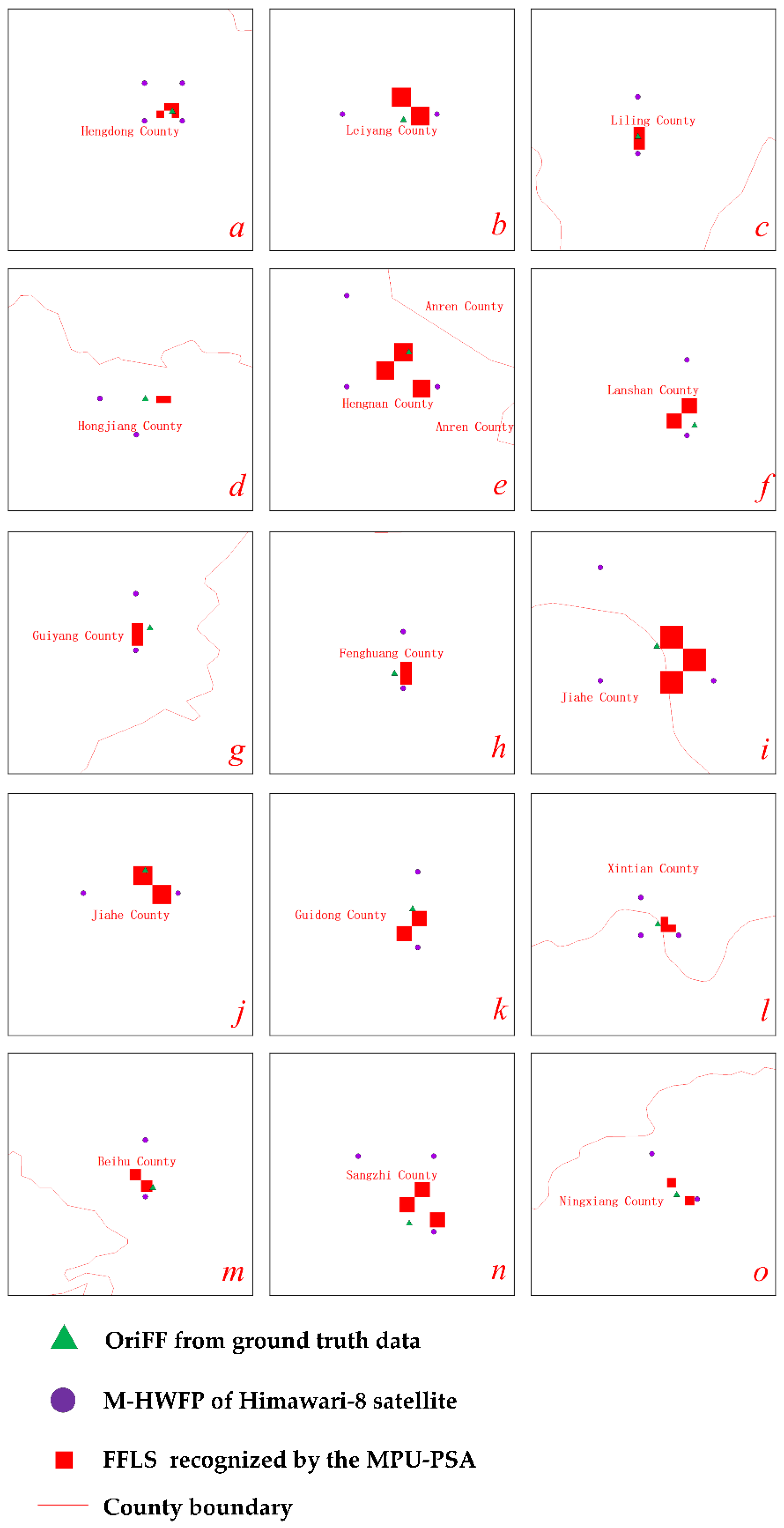
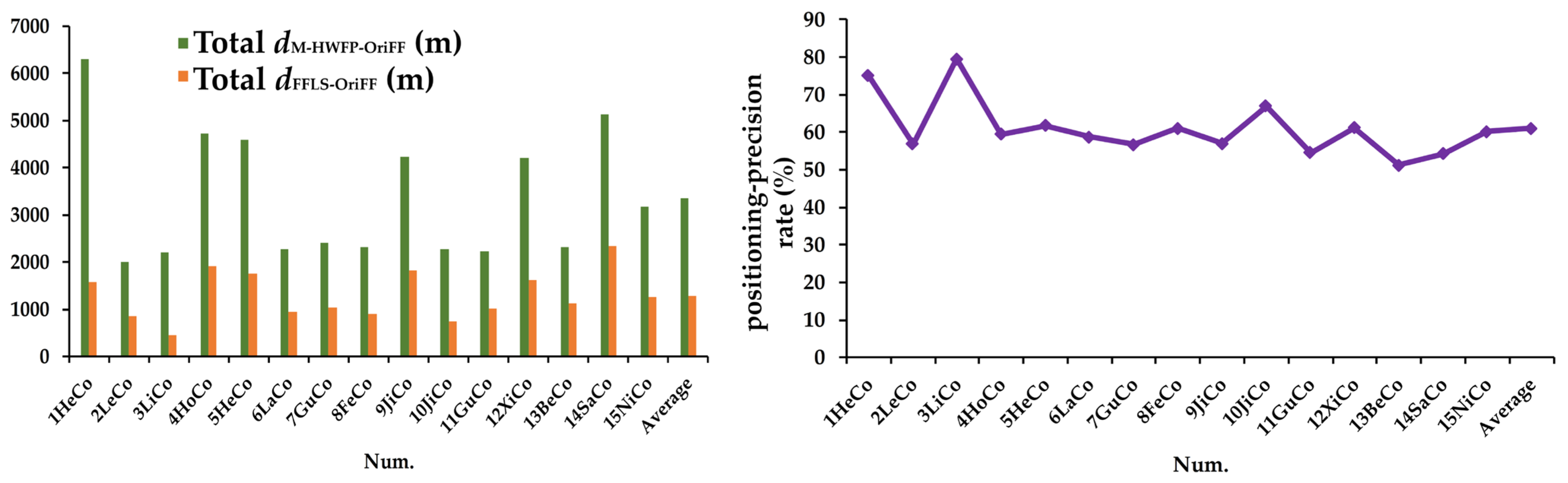
3.2. Comparison of M-HWFP and FFLS in Positioning Accuracy

Comparative analysis results from d_M-HWFP-OriFF and d_FFLS-OriFF indices data are shown in

Table 2. Positioning-accuracy comparison of M-HWFP to OriFF and FFLS to OriFF. PPR represents positioning-precision rate.

Num.	Easting and Northing						Total dM-HWFP-OriFF (m)	Total dFFLS-OriFF (m)	PPR (%)
	OriFF		M-HWFP		FFLS
	Easting (m)	Northing (m)	Easting (m)	Northing (m)	Easting (m)	Northing (m)
1HeCo	705,596.58	3,006,410.92	704,082.66	3,008,048.47	704,954.05	3,006,231.03	6294.90	1573.00	75.01
	705,596.58	3,006,410.92	706,064.56	3,008,081.20	705,343.10	3,006,680.72
	705,596.58	3,006,410.92	704,119.06	3,005,832.40	705,739.46	3,006,687.27
	705,596.58	3,006,410.92	706,101.31	3,005,865.10	705,746.79	3,006,244.13
2LeCo	702,756.60	2,923,687.72	701,458.01	2,923,778.10	702,698.15	2,924,196.13	2008.86	866.57	56.86
	702,756.60	2,923,687.72	703,453.15	2,923,809.56	703,104.11	2,923,759.34
3LiCo	731,319.58	3,035,796.60	731,290.37	3,037,348.07	731,360.44	3,035,955.75	2216.78	452.59	79.58
	731,319.58	3,035,796.60	731,332.09	3,035,131.68	731,368.78	3,035,512.54
4HoCo	389,661.48	3,015,656.00	387,151.62	3,015,747.42	390,419.76	3,015,657.80	4722.92	1912.50	59.51
	389,661.48	3,015,656.00	389,111.73	3,013,514.02	390,815.69	3,015,654.38
5HeCo	708,216.34	2,960,200.00	706,831.09	2,961,544.35	707,705.02	2,959,734.72	4592.03	1754.73	61.79
	708,216.34	2,960,200.00	706,867.31	2,959,328.37	708,095.58	2,960,184.38
	708,216.34	2,960,200.00	708,856.95	2,959,361.04	708,508.02	2,959,304.68
6LaCo	630,975.42	2,807,970.71	630,761.87	2,809,876.75	630,434.73	2,808,518.79	2281.77	942.67	58.69
	630,975.42	2,807,970.71	630,783.42	2,807,661.70	630,841.40	2,808,079.76
7GuCo	688,789.37	2,866,830.81	688,294.29	2,868,175.04	688,365.96	2,866,811.21	2419.37	1046.73	56.74
	688,789.37	2,866,830.81	688,326.07	2,865,959.45	688,372.32	2,866,368.16
8FeCo	369,975.51	3,102,917.48	370,279.78	3,104,551.89	370,363.30	3,102,703.42	2307.95	897.46	61.11
	369,975.51	3,102,917.48	370,255.77	3,102,336.03	370,368.09	3,103,146.51
9JiCo	631,515.70	2,846,529.30	630,393.03	2,847,533.50	631,671.98	2,846,185.04	4242.42	1821.94	57.05
	631,515.70	2,846,529.30	630,414.86	2,845,318.35	631,680.80	2,845,299.13
	631,515.70	2,846,529.30	632,421.46	2,845,338.26	632,077.63	2,845,746.08
10JiCo	645,860.26	2,839,339.22	644,533.72	2,838,818.48	645,793.16	2,839,244.63	2269.30	747.91	67.04
	645,860.26	2,839,339.22	646,541.41	2,838,840.48	646,199.49	2,838,806.07
11GuCo	790,268.92	2,875,627.18	790,351.29	2,876,689.63	790,025.81	2,874,871.95	2230.77	1013.74	54.56
	790,268.92	2,875,627.18	790,400.46	2,874,473.01	790,416.67	2,875,324.08
12XiCo	631,319.73	2,845,985.37	630,393.03	2,847,533.50	631,671.99	2,846,185.04	4206.16	1631.44	61.21
	631,319.73	2,845,985.37	630,414.86	2,845,318.35	631,676.40	2,845,742.08
	631319.73	2,845,985.37	632,421.46	2,845,338.26	632,077.64	2,845,746.07
13BeCo	687,060.14	2,844,208.01	686,604.09	2,845,990.97	686,280.65	2,844,182.18	2320.74	1130.68	51.28
	687,060.14	2,844,208.01	686,635.30	2,843,775.45	686,675.78	2,844,630.86
14SaCo	404,309.30	3,255,150.96	403,012.85	3,257,151.48	405,033.63	3,255,261.12	5136.11	2351.74	54.21
	404,309.30	3,255,150.96	404,952.70	3,257,135.00	404,653.13	3,256,150.69
	404,309.30	3,255,150.96	404,934.07	3,254,918.86	404,261.44	3,255,710.81
15NiCo	599,212.52	3,119,992.26	598,124.89	3,121,978.22	598,986.92	3,120,578.12	3183.05	1266.23	60.22
	599,212.52	3,119,992.26	600,106.15	3,119,778.82	599,779.36	3,119,698.53
Average							3362.21	1294.00	60.99

to illustrate the better performance of FFLS in comparison with M-HWFP in locating forest fires. M-HWFP provides the pixel-level fire locations, which were retrieved from the infrared band (IR) images of the Himawari-8 satellite using the method developed by JAXA/EORC [63,64]. Using the proposed method, we attempted to obtain more precise spatial locations of OriFFs than those obtained using traditional forest-fire detection methods, such as M-HWFP. Knowing the exact locations of forest fires is imperative in effective forestry firefighting, especially in virgin and dense forests among high mountains with bumpy or even no roads. As shown in Table 2, the coordinates of fire locations are projected coordinates with easting and northing in meters. Taking the first forest-fire event (i.e., 1HeCo) as an example, TCFI data showed that the forest fire started at 12:00 UTC on 24 September 2019, and the closest timepoint to forest-fire starting time recorded by Himawari-8 satellite was 11:30 UTC on 24 September 2019. In Table 2, d_M-HWFP-OriFF and d_FFLS-OriFF are 6294.90 m and 1573.00 m, respectively. Therefore, for the first forest-fire event (i.e., 1HeCo), the FFLS-estimated OriFF was closer to the actual OriFF than the M-HWFP-estimated OriFF, with a positioning-precision rate of 75.01%.

As shown in Figure 7 and Table 2, the positioning-precision rates of the fifteen forest-fire events all exceeded 50%. The mean d_M-HWFP-OriFF, d_FFLS-OriFF, and positioning-precision rate were 3362.21 m, 1294.00 m, and 60.99%, respectively. The largest positioning-precision rate was 79.58%, and the lowest positioning-precision rate was 51.28%. The positioning-precision rates of two forest-fire events exceeded 70.00%, and the positioning-precision rates of five forest-fire events exceeded 60.00%. The MPU-PSA method has an advantage in monitoring OriFFs over the traditional forest-fire detection method.

3.3. Accuracy Comparison between M-HWFP and FFLS

We chose two commonly used accuracy-evaluation indexes, RMSE and MAE, to evaluate the accuracy of M-HWFP and FFLS. Compared with M-HWFP, FFLS showed more accurate spatial location of OriFFs.

Table 3. Accuracy comparison of M-HWFP and FFLS.

Num.	RMSE			MAE
	M-HWFP (m)	FFLS (m)	Decrease of RMSE (%)	M-HWFP (m)	FFLS (m)	Decrease of MAE (%)
1HeCo	1486.79	381.95	74.31	1258.98	314.60	75.01
2LeCo	855.29	359.53	57.96	669.62	288.86	56.86
3LiCo	1193.77	234.63	80.35	1108.39	226.30	79.58
4HoCo	1673.17	690.51	58.73	1180.73	478.13	59.51
5HeCo	1218.20	525.25	56.88	918.41	350.95	61.79
6LaCo	1380.39	557.94	59.58	1140.88	471.34	58.69
7GuCo	1230.04	532.74	56.69	1209.69	523.37	56.74
8FeCo	891.70	317.33	64.41	576.99	224.36	61.11
9JiCo	1251.74	550.63	56.01	1060.61	455.49	57.06
10JiCo	740.75	287.33	61.21	453.86	149.58	67.04
11GuCo	596.27	295.13	50.50	318.68	144.82	54.56
12XiCo	1240.13	495.49	60.05	1051.54	407.86	61.21
13BeCo	1345.00	568.12	57.76	1160.37	565.34	51.28
14SaCo	1868.81	810.39	56.64	1712.04	783.91	54.21
15NiCo	1410.81	516.95	63.36	1061.02	422.08	60.22
Average	1225.52	474.93	60.96	992.12	387.13	60.99

shows RMSE and MAE values of M-HWFP and FFLS datasets for the fifteen forest-fire events. Taking the first forest-fire event (i.e., 1HeCo) as an example, M-HWFP has RMSE = 1486.79 m and MAE = 1258.98 m, while FFLS produced by the MPU-PSA method has RMSE = 381.95 m, decreased by 74.31%; and MAE = 314.60 m, decreased by 75.01%. As shown in Table 3, the largest decreases in RMSE and MAE were 80.35% and 79.58%, respectively; and the smallest decreases in RMSE and MAE were 50.50% and 51.28%, respectively. For the 15 reference forest-fire events, the decrease in RMSE and MAE exceeded 50.00%. There was one forest-fire event with an RMSE decrease exceeding 80.00%, and there were six forest-fire events with RMSE decrease exceeding 60.00%. There were two forest-fire events with an MAE decrease exceeding 70.00%, and seven forest-fire events with an MAE decrease exceeding 60.00%. Furthermore, the average RMSE and MAE of M-HWFP were 1225.52 m and 992.12 m, respectively, owing to the low spatial resolution of the Himawari-8 satellite. On the other hand, the average RMSE and MAE of FFLS were 474.93 m and 387.13 m, respectively. FFLS generally showed a more refined detection of spatial location of forest fires than M-HWFP.

4. Discussion

Traditionally, forest-fire detection has mainly relied on artificial ground patrols and watchtowers [65]. Slow acquisition of fire information, such as location and starting time, using the conventional methods often lead to delayed action and ultimately to forest-fire disasters. The advent of remote-sensing techniques, such as satellite-based [66,67], aerial-based [68], and ground-surveillance-camera-based [69] techniques, offers researchers alternative or even better methods for forest-fire detection and monitoring. Meteorological satellites are widely used in forest-fire detection and monitoring because of their high temporal resolution. For example, Jang et al. [13] detected most forest fires successfully based on the Himawari-8 satellite data. In this study, we could monitor and detect forest fires every 10 min using the Himawari-8 satellite data. The high temporal resolution makes it possible to detect forest fires in almost real time.

However, forest-fire monitoring at pixel scale can cause large errors in fire locations. The ability of subpixels to specify the distribution location of mixed pixel composition could somewhat improve this situation [31,32]. Burnt-area estimation at subpixel level using Advanced Very-High-Resolution Radiometer (AVHRR) data has a mean error of 6.5% [70]. In this study, we proposed the MPU-PSA method to detect OriFFs. Compared with M-HWFP, OriFF detection by the new method (MPU-PSA) has higher positioning accuracy. On the one hand, the subpixel result (i.e., FFLS) maintains the high temporal resolution of the Himawari-8 satellite but provides more accurate positions of forest fires. Identification of fire locations at subpixel level enhanced forest-fire monitoring. It is of great importance that forest fires are extinguished in a timely manner at their OriFF locations. The MPU-PSA method was successfully applied to fifteen forest fires in Hunan province, China. However, in future research, it should be a priority to carry out research to validate and conduct the MPU-PSA in other regions. Furthermore, it is necessary to further improve forest-fire positioning accuracy at subpixel scale by improving the algorithm.

5. Conclusions

In this study, we proposed a forest-fire detection model for forest-fire detection at subpixel level (MPU-PSA), and applied the model to the Himawari-8 satellite data for fire detection. The proposed model involves two main procedures: (1) pixel-unmixing analysis to obtain forest-fire distribution, and (2) adaptation of the pixel-swapping algorithm to generate the FFLS dataset for OriFF estimation. The MPU-PSA method was applied to fifteen forest-fire events occurring in Hunan Province, China. Compared with the M-HWFP product, the FFLS dataset has better positioning accuracy, which was reflected in three accuracy-evaluation indices: Euclidean Distance, RMSE, and MAE. Positioning error was significantly improved, decreasing from 3362.21 m to 1294.00 m (with the average positioning-precision rate being 60.99%). The mean RMSE decreased from 1225.52 m to 474.93 m (decrease rate = 60.96%), and the mean MAE decreased from 992.12 m to 387.13 m (decrease rate = 60.99%). All these results show that (1) the MPU-PSA method developed in this study can estimate forest-fire locations at subpixel level, which is more accurate than the conventional pixel-level method, especially for geostationary satellite products, such as the Himawari-8 Wild Fire Product, which has low spatial resolution but high temporal resolution, and (2) the FFLS product with geographic information can provide more accurate OriFF locations than the M-HWFP product. This new forest-fire detection technique can assist in forest-fire extinguishment by quickly and accurately detecting OriFF locations.

References

1. Administration, N.F. (Ed.) National Forest Fire Prevention Plan (2016–2025); FAO: Beijing, China, 2016. [Google Scholar]
2. Sannigrahi, S.; Pilla, F.; Basu, B.; Basu, A.S.; Sarkar, K.; Chakraborti, S.; Joshi, P.K.; Zhang, Q.; Wang, Y.; Bhatt, S.; et al. Examining the effects of forest fire on terrestrial carbon emission and ecosystem production in India using remote sensing approaches. Sci. Total Environ. 2020, 725, 138331. [Google Scholar] [CrossRef] [PubMed]
3. Fernandez-Carrillo, A.; McCaw, L.; Tanase, M.A. Estimating prescribed fire impacts and post-fire tree survival in eucalyptus forests of Western Australia with L-band SAR data. Remote Sens. Environ. 2019, 224, 133–144. [Google Scholar] [CrossRef]
4. Matin, M.A.; Chitale, V.S.; Murthy, M.S.R.; Uddin, K.; Bajracharya, B.; Pradhan, S. Understanding forest fire patterns and risk in Nepal using remote sensing, geographic information system and historical fire data. Int. J. Wildland Fire 2017, 26, 276–286. [Google Scholar] [CrossRef] [Green Version]
5. Forest Fire in Sichuan Province, China in 2019. 4 April 2019. Available online: http://www.lsz.gov.cn/ztzl/lszt/2019ztzl/mlxslhztbbd/yw/201904/t20190404_1171588.html (accessed on 24 December 2021). (In Chinese)
6. Forest Fire in Sichuan Province, China in 2020. 31 March 2020. Available online: http://www.xuezhangbb.com/news/tag/67379390 (accessed on 24 December 2021). (In Chinese).
7. Forest Fire in Sichuan Province, China in 2021. 20 April 2021. Available online: https://baike.baidu.com/item/4%C2%B720%E5%86%95%E5%AE%81%E6%A3%AE%E6%9E%97%E7%81%AB%E7%81%BE/56798303?fr=aladdin (accessed on 24 December 2021). (In Chinese).
8. Jolly, C.; Nimmo, D.; Dickman, C.; Legge, S.; Woinarski, J. Estimating Wildlife Mortality during the 2019–20 Bushfire Season; NESP Threatened Sprecies Recovery Hub Project 8.3.4 Report; NESP: Brisbane, Australia, 2021. [Google Scholar]
9. De Bem, P.P.; de Carvalho Júnior, O.A.; Matricardi, E.A.T.; Guimarães, R.F.; Gomes, R.A.T. Predicting wildfire vulnerability using logistic regression and artificial neural networks: A case study in Brazil’s Federal District. Int. J. Wildland Fire 2019, 28, 35–45. [Google Scholar] [CrossRef]
10. Cardil, A.; Monedero, S.; Ramirez, J.; Silva, C.A. Assessing and reinitializing wildland fire simulations through satellite active fire data. J. Environ. Manag. 2019, 231, 996–1003. [Google Scholar] [CrossRef]
11. Dwomoh, F.K.; Wimberly, M.C.; Cochrane, M.A.; Numata, I. Forest degradation promotes fire during drought in moist tropical forests of Ghana. For. Ecol. Manag. 2019, 440, 158–168. [Google Scholar] [CrossRef]
12. He, Y.; Chen, G.; De Santis, A.; Roberts, D.A.; Zhou, Y.; Meentemeyer, R.K. A disturbance weighting analysis model (DWAM) for mapping wildfire burn severity in the presence of forest disease. Remote Sens. Environ. 2019, 221, 108–121. [Google Scholar] [CrossRef]
13. Jang, E.; Kang, Y.; Im, J.; Lee, D.-W.; Yoon, J.; Kim, S.-K. Detection and Monitoring of Forest Fires Using Himawari-8 Geostationary Satellite Data in South Korea. Remote Sens. 2019, 11, 271. [Google Scholar] [CrossRef] [Green Version]
14. Filizzola, C.; Corrado, R.; Marchese, F.; Mazzeo, G.; Paciello, R.; Pergola, N.; Tramutoli, V. RST-FIRES, an exportable algorithm for early-fire detection and monitoring: Description, implementation, and field validation in the case of the MSG-SEVIRI sensor. Remote Sens. Environ. 2016, 186, 196–216. [Google Scholar] [CrossRef]
15. Tien Bui, D.; Hoang, N.D.; Samui, P. Spatial pattern analysis and prediction of forest fire using new machine learning approach of Multivariate Adaptive Regression Splines and Differential Flower Pollination optimization: A case study at Lao Cai province (Viet Nam). J. Environ. Manag. 2019, 237, 476–487. [Google Scholar] [CrossRef]
16. Xie, Z.; Song, W.; Ba, R.; Li, X.; Xia, L. A Spatiotemporal Contextual Model for Forest Fire Detection Using Himawari-8 Satellite Data. Remote Sens. 2018, 10, 1992. [Google Scholar] [CrossRef] [Green Version]
17. Vikram, R.; Sinha, D.; De, D.; Das, A.K. EEFFL: Energy efficient data forwarding for forest fire detection using localization technique in wireless sensor network. Wirel. Netw. 2020, 26, 5177–5205. [Google Scholar] [CrossRef]
18. Kaur, I.; Hüser, I.; Zhang, T.; Gehrke, B.; Kaiser, J. Correcting Swath-Dependent Bias of MODIS FRP Observations With Quantile Mapping. Remote Sens. 2019, 11, 1205. [Google Scholar] [CrossRef] [Green Version]
19. Hua, L.; Shao, G. The progress of operational forest fire monitoring with infrared remote sensing. J. For. Res. 2016, 28, 215–229. [Google Scholar] [CrossRef]
20. Dozier, J. A Method for Satellite Identification of Surface Temperature Fields of Subpixel Resolution. Remote Sens. Environ. 1981, 11, 221–229. [Google Scholar] [CrossRef]
21. Eckmann, T.; Roberts, D.; Still, C. Using multiple endmember spectral mixture analysis to retrieve subpixel fire properties from MODIS. Remote Sens. Environ. 2008, 112, 3773–3783. [Google Scholar] [CrossRef]
22. Zhukov, B.; Lorenz, E.; Oertel, D.; Wooster, M.; Roberts, G. Spaceborne detection and characterization of fires during the bi-spectral infrared detection (BIRD) experimental small satellite mission (2001–2004). Remote Sens. Environ. 2006, 100, 29–51. [Google Scholar] [CrossRef]
23. Giglio, L.; Schroeder, W. A global feasibility assessment of the bi-spectral fire temperature and area retrieval using MODIS data. Remote Sens. Environ. 2014, 152, 166–173. [Google Scholar] [CrossRef] [Green Version]
24. Kaufman, Y.J.; Tucker, C.J.; Fung, I.Y. Remote sensing of biomass burning in the tropics. J. Geophys. Res. 1990, 95, 9927–9939. [Google Scholar] [CrossRef]
25. Giglio, L.; Schroeder, W.; Justice, C.O. The collection 6 MODIS active fire detection algorithm and fire products. Remote Sens. Environ. 2016, 178, 31–41. [Google Scholar] [CrossRef] [Green Version]
26. Lin, Z.; Chen, F.; Niu, Z.; Li, B.; Yu, B.; Jia, H.; Zhang, M. An active fire detection algorithm based on multi-temporal FengYun-3C VIRR data. Remote Sens. Environ. 2018, 211, 376–387. [Google Scholar] [CrossRef]
27. Robinson, J.M. Fire from space: Global fire evaluation using infrared remote sensing. Int. J. Remote Sens. 2007, 12, 3–24. [Google Scholar] [CrossRef]
28. Roberts, G.; Wooster, M.J. Development of a multi-temporal Kalman filter approach to geostationary active fire detection & fire radiative power (FRP) estimation. Remote Sens. Environ. 2014, 152, 392–412. [Google Scholar] [CrossRef]
29. Moreno, M.V.; Laurent, P.; Ciais, P.; Mouillot, F. Assessing satellite-derived fire patches with functional diversity trait methods. Remote Sens. Environ. 2020, 247, 111897. [Google Scholar] [CrossRef]
30. Liu, X.; He, B.; Quan, X.; Yebra, M.; Qiu, S.; Yin, C.; Liao, Z.; Zhang, H. Near Real-Time Extracting Wildfire Spread Rate from Himawari-8 Satellite Data. Remote Sens. 2018, 10, 1654. [Google Scholar] [CrossRef] [Green Version]
31. Atkinson, P.M. Mapping Sub-Pixel Boundaries from Remotely Sensed Images; Taylor and Francis: London, UK, 1997; Volume 4, pp. 166–180. [Google Scholar]
32. Atkinson, P.M.; Cutler, M.E.J.; Lewis, H. Mapping sub-pixel proportional land cover with AVHRR imagery. Int. J. Remote Sens. 1997, 18, 917–935. [Google Scholar] [CrossRef]
33. Wang, Q.; Zhang, C.; Atkinson, P.M. Sub-pixel mapping with point constraints. Remote Sens. Environ. 2020, 244, 111817. [Google Scholar] [CrossRef]
34. Wu, S.; Ren, J.; Chen, Z.; Jin, W.; Liu, X.; Li, H.; Pan, H.; Guo, W. Influence of reconstruction scale, spatial resolution and pixel spatial relationships on the sub-pixel mapping accuracy of a double-calculated spatial attraction model. Remote Sens. Environ. 2018, 210, 345–361. [Google Scholar] [CrossRef]
35. Yu, W.; Li, J.; Liu, Q.; Zeng, Y.; Zhao, J.; Xu, B.; Yin, G. Global Land Cover Heterogeneity Characteristics at Moderate Resolution for Mixed Pixel Modeling and Inversion. Remote Sens. 2018, 10, 856. [Google Scholar] [CrossRef] [Green Version]
36. He, Y.; Yang, J.; Guo, X. Green Vegetation Cover Dynamics in a Heterogeneous Grassland: Spectral Unmixing of Landsat Time Series from 1999 to 2014. Remote Sens. 2020, 12, 3826. [Google Scholar] [CrossRef]
37. Shao, Y.; Lan, J. A Spectral Unmixing Method by Maximum Margin Criterion and Derivative Weights to Address Spectral Variability in Hyperspectral Imagery. Remote Sens. 2019, 11, 1045. [Google Scholar] [CrossRef] [Green Version]
38. Craig, M.D. Minimum-Volume Transforms for Remotely Sensed Data. IEEE Trans. Geosci. Remote Sens. 1994, 32, 542–552. [Google Scholar] [CrossRef]
39. Nascimento, J.M.P.; Dias, J.M.B. Vertex component analysis: A fast algorithm to unmix hyperspectral data. IEEE Trans. Geosci. Remote Sens. 2005, 43, 898–910. [Google Scholar] [CrossRef] [Green Version]
40. Chang, C.I.; Wu, C.C.; Liu, W.; Ouyang, Y.C. A New Growing Method for Simplex-Based Endmember Extraction Algorithm. IEEE Trans. Geosci. Remote Sens. 2006, 44, 2804–2819. [Google Scholar] [CrossRef]
41. Miao, L.; Qi, H. Endmember Extraction From Highly Mixed Data Using Minimum Volume Constrained Nonnegative Matrix Factorization. IEEE Trans. Geosci. Remote Sens. 2007, 45, 765–777. [Google Scholar] [CrossRef]
42. Zhang, J.; Rivard, B.; Rogge, D.M. The Successive Projection Algorithm (SPA), an Algorithm with a Spatial Constraint for the Automatic Search of Endmembers in Hyperspectral Data. Sensors 2008, 8, 1321–1342. [Google Scholar] [CrossRef] [PubMed] [Green Version]
43. Winter, M.E. N-FINDR: An algorithm for fast autonomous spectral end-member determination in hyperspectral data. In Proceedings of the SPIE Conference on lmacjincj Spectrometry V, Denver, CO, USA, 18–23 July 1999; pp. 266–275. [Google Scholar]
44. Atkinson, P.M. Sub-pixel Target Mapping from Soft-classified, Remotely Sensed Imagery. Photogramm. Eng. Remote Sens. 2005, 71, 839–846. [Google Scholar] [CrossRef] [Green Version]
45. Wang, Q.M.; Atkinson, P.M. The effect of the point spread function on sub-pixel mapping. Remote Sens. Environ. 2017, 193, 127–137. [Google Scholar] [CrossRef] [Green Version]
46. Kumar, U.; Ganguly, S.; Nemani, R.R.; Raja, K.S.; Milesi, C.; Sinha, R.; Michaelis, A.; Votava, P.; Hashimoto, H.; Li, S.; et al. Exploring Subpixel Learning Algorithms for Estimating Global Land Cover Fractions from Satellite Data Using High Performance Computing. Remote Sens. 2017, 9, 1105. [Google Scholar] [CrossRef] [Green Version]
47. Wang, Y.; Chen, Q.; Ding, M.; Li, J. High Precision Dimensional Measurement with Convolutional Neural Network and Bi-Directional Long Short-Term Memory (LSTM). Sensors 2019, 19, 5302. [Google Scholar] [CrossRef] [Green Version]
48. Hu, C. A novel ocean color index to detect floating algae in the global oceans. Remote Sens. Environ. 2009, 113, 2118–2129. [Google Scholar] [CrossRef]
49. Salomonson, V.V.; Appel, I. Estimating fractional snow cover from MODIS using the normalized difference snow index. Remote Sens. Environ. 2004, 89, 351–360. [Google Scholar] [CrossRef]
50. Salomonson, V.V.; Appel, I. Development of the Aqua MODIS NDSI fractional snow cover algorithm and validation results. IEEE Trans. Geosci. Remote Sens. 2006, 44, 1747–1756. [Google Scholar] [CrossRef]
51. He, Y.; Chen, G.; Potter, C.; Meentemeyer, R.K. Integrating multi-sensor remote sensing and species distribution modeling to map the spread of emerging forest disease and tree mortality. Remote Sens. Environ. 2019, 231, 111238. [Google Scholar] [CrossRef]
52. Li, L.; Chen, Y.; Xu, T.; Shi, K.; Liu, R.; Huang, C.; Lu, B.; Meng, L. Remote Sensing of Wetland Flooding at a Sub-Pixel Scale Based on Random Forests and Spatial Attraction Models. Remote Sens. 2019, 11, 1231. [Google Scholar] [CrossRef] [Green Version]
53. Li, X.; Chen, R.; Foody, G.M.; Wang, L.; Yang, X.; Du, Y.; Ling, F. Spatio-Temporal Sub-Pixel Land Cover Mapping of Remote Sensing Imagery Using Spatial Distribution Information From Same-Class Pixels. Remote Sens. 2020, 12, 503. [Google Scholar] [CrossRef] [Green Version]
54. Ling, F.; Li, X.; Foody, G.M.; Boyd, D.; Ge, Y.; Li, X.; Du, Y. Monitoring surface water area variations of reservoirs using daily MODIS images by exploring sub-pixel information. ISPRS J. Photogramm. Remote Sens. 2020, 168, 141–152. [Google Scholar] [CrossRef]
55. Deng, C.; Zhu, Z. Continuous subpixel monitoring of urban impervious surface using Landsat time series. Remote Sens. Environ. 2020, 238, 110929. [Google Scholar] [CrossRef]
56. Bessho, K.; Date, K.; Hayashi, M.; Ikeda, A.; Imai, T.; Inoue, H.; Kumagai, Y.; Miyakawa, T.; Murata, H.; Ohno, T.; et al. An Introduction to Himawari-8/9—Japan’s New-Generation Geostationary Meteorological Satellites. J. Meteorol. Soc. Japan. Ser. II 2016, 94, 151–183. [Google Scholar] [CrossRef] [Green Version]
57. Zhang, X.; Zhang, Q.; Zhang, G.; Nie, Z.; Gui, Z.; Que, H. A Novel Hybrid Data-Driven Model for Daily Land Surface Temperature Forecasting Using Long Short-Term Memory Neural Network Based on Ensemble Empirical Mode Decomposition. Int. J. Environ. Res. Public Health 2018, 15, 1032. [Google Scholar] [CrossRef] [Green Version]
58. Wang, F.; Yang, M.; Ma, L.; Zhang, T.; Qin, W.; Li, W.; Zhang, Y.; Sun, Z.; Wang, Z.; Li, F.; et al. Estimation of Above-Ground Biomass of Winter Wheat Based on Consumer-Grade Multi-Spectral UAV. Remote Sens. 2022, 14, 1251. [Google Scholar] [CrossRef]
59. Vafaei, S.; Soosani, J.; Adeli, K.; Fadaei, H.; Naghavi, H.; Pham, T.; Tien Bui, D. Improving Accuracy Estimation of Forest Aboveground Biomass Based on Incorporation of ALOS-2 PALSAR-2 and Sentinel-2A Imagery and Machine Learning: A Case Study of the Hyrcanian Forest Area (Iran). Remote Sens. 2018, 10, 172. [Google Scholar] [CrossRef] [Green Version]
60. Chai, T.; Draxler, R.R. Root mean square error (RMSE) or mean absolute error (MAE)?—Arguments against avoiding RMSE in the literature. Geosci. Model Dev. 2014, 7, 1247–1250. [Google Scholar] [CrossRef] [Green Version]
61. Li, H.; Kato, T.; Hayashi, M.; Wu, L. Estimation of Forest Aboveground Biomass of Two Major Conifers in Ibaraki Prefecture, Japan, from PALSAR-2 and Sentinel-2 Data. Remote Sens. 2022, 14, 468. [Google Scholar] [CrossRef]
62. An, G.; Xing, M.; He, B.; Liao, C.; Huang, X.; Shang, J.; Kang, H. Using Machine Learning for Estimating Rice Chlorophyll Content from In Situ Hyperspectral Data. Remote Sens. 2020, 12, 3104. [Google Scholar] [CrossRef]
63. Kurihara, Y.; Tanada, K.; Murakami, H.; Kachi, M. Australian bushfire captured by AHI/Himawari-8 and SGLI/GCOM-C. In Proceedings of the JpGU-AGU Joint Meeting 2020, Chiba, Japan, 24–28 May 2020. [Google Scholar]
64. JAXA Himawari Monitor User’s Guide. Available online: https://www.eorc.jaxa.jp/ptree/userguide.html (accessed on 26 December 2021).
65. Wu, X.; Gao, N.; Zheng, X.; Tao, X.; He, Y.; Liu, Z.; Wang, Y. Self-Powered and Green Ionic-Type Thermoelectric Paper Chips for Early Fire Alarming. ACS Appl. Mater. Interfaces 2020, 12, 27691–27699. [Google Scholar] [CrossRef] [PubMed]
66. Yao, J.; Raffuse, S.M.; Brauer, M.; Williamson, G.J.; Bowman, D.M.J.S.; Johnston, F.H.; Henderson, S.B. Predicting the minimum height of forest fire smoke within the atmosphere using machine learning and data from the CALIPSO satellite. Remote Sens. Environ. 2018, 206, 98–106. [Google Scholar] [CrossRef]
67. Li, X.; Song, W.; Lian, L.; Wei, X. Forest Fire Smoke Detection Using Back-Propagation Neural Network Based on MODIS Data. Remote Sens. 2015, 7, 4473–4498. [Google Scholar] [CrossRef] [Green Version]
68. Ciullo, V.; Rossi, L.; Pieri, A. Experimental Fire Measurement with UAV Multimodal Stereovision. Remote Sens. 2020, 12, 3546. [Google Scholar] [CrossRef]
69. Rosas-Romero, R. Remote detection of forest fires from video signals with classifiers based on K-SVD learned dictionaries. Eng. Appl. Artif. Intell. 2014, 33, 53. [Google Scholar] [CrossRef]
70. Ruescas, A.B.; Sobrino, J.A.; Julien, Y.; Jiménez-Muñoz, J.C.; Sòria, G.; Hidalgo, V.; Atitar, M.; Franch, B.; Cuenca, J.; Mattar, C. Mapping sub-pixel burnt percentage using AVHRR data. Application to the Alcalaten area in Spain. Int. J. Remote Sens. 2010, 31, 5315–5330. [Google Scholar] [CrossRef]
Figure 1. Flowchart of the analysis performed in the current study. M-HWFP represents modified Himawari-8 Wild Fire Product. MPU-PSA represents mixed-pixel unmixing integrated with pixel-swapping algorithm. FFLS represents forest-fire locations at subpixel. RMSE represents root mean square error. MAE represents mean absolute error.
Remotesensing 14 02460 g001
Figure 2. Location of the study area. (a) Study boundary within China for which data were downloaded http://bzdt.ch.mnr.gov.cn/ (accessed on 10 December 2021), (b) the 15 forest-fire events in Hunan Province, China as reference data.
Remotesensing 14 02460 g002
Figure 3. Determination of M-HWFP and preprocessed HLGD datasets pertaining to the time closest to a forest fire’s starting time in a target area. (a) Red points represent hotspots derived from the HWFP data. (b) UTC times when the forest-fire events were detected by Himawari-8 satellite are shown in the first red circle; the earliest UTC times when the forest-fire events were detected by Himawari-8 satellite are shown in the 2nd red circle; the number of times a forest-fire event was detected in a day is shown in the 3rd red circle.
Remotesensing 14 02460 g003
Figure 4. Field measurements to confirm and report forest-fire information. (a,b) Forest-fire sites located in Hunan Province, China. (c) Well-trained personal confirmed and reported forest-fire information.
Remotesensing 14 02460 g004
Figure 5. Positioning-accuracy comparison between M-HWFP and FFLS in detecting fire locations in various counties. OriFF represents origin of forest fire. The location-detection of the forest fires occurred in (a) Hengdong County (1HeCo), (b) Leiyang County (2LeCo), (c) Liling County (3LiCo), (d) Hongjiang County (4HoCo), (e) the junction of Hengnan County and Anren County (5HeCo), (f) Lanshan County (6LaCo), (g) Guiyang County (7GuCo), (h) Fenghuang County (8FeCo), (i) Jiahe County (9JiCo), (j) Jiahe County (10JiCo), (k) Guidong County (11GuCo), (l) Xintian County (12XiCo), (m) Beihu County (13BeCo), (n) Sangzhi County (14SaCo), and (o) Ningxiang County (15NiCo).
Remotesensing 14 02460 g005
Figure 6. Locations of fifteen forest-fire events detected at subpixel level by the new MPU-PSA method. The improved location-detection of the forest fires occurred in (a) Hengdong County (1HeCo), (b) Leiyang County (2LeCo), (c) Liling County (3LiCo), (d) Hongjiang County (4HoCo), (e) the junction of Hengnan County and Anren County (5HeCo), (f) Lanshan County (6LaCo), (g) Guiyang County (7GuCo), (h) Fenghuang County (8FeCo), (i) Jiahe County (9JiCo), (j) Jiahe County (10JiCo), (k) Guidong County (11GuCo), (l) Xintian County (12XiCo), (m) Beihu County (13BeCo), (n) Sangzhi County (14SaCo), and (o) Ningxiang County (15NiCo).
Remotesensing 14 02460 g006
Figure 7. Positioning-accuracy comparison of M-HWFP to OriFF and FFLS to OriFF.
Remotesensing 14 02460 g007