Article

Leveraging Machine Learning and Geo-Tagged Citizen Science Data to Disentangle the Factors of Avian Mortality Events at the Species Level

1
Department of Geography and Environmental Sustainability, University of Oklahoma, Norman, OK 73019, USA
2
Wyoming Geographic Information Science Center, University of Wyoming, Laramie, WY 82071, USA
3
Department of Geography, University of Georgia, Athens, GA 30602, USA
4
Division of Landscape Architecture, College of Architecture, University of Oklahoma, Norman, OK 73019, USA
5
Department of Occupational and Environmental Health, The University of Oklahoma Health Sciences Center, University of Oklahoma, Oklahoma City, OK 73126, USA
6
Atmospheric Sciences and Global Change Division, Pacific Northwest National Laboratory, Richland, WA 99352, USA
*
Author to whom correspondence should be addressed.
Remote Sens. 2022, 14(10), 2369; https://doi.org/10.3390/rs14102369
Submission received: 25 February 2022 / Revised: 20 April 2022 / Accepted: 11 May 2022 / Published: 14 May 2022
(This article belongs to the Section Environmental Remote Sensing)

Abstract

:
Abrupt environmental changes can affect the population structures of living species and cause habitat loss and fragmentations in the ecosystem. During August–October 2020, remarkably high mortality events of avian species were reported across the western and central United States, likely resulting from winter storms and wildfires. However, the differences of mortality events among various species responding to the abrupt environmental changes remain poorly understood. In this study, we focused on three species, Wilson’s Warbler, Barn Owl, and Common Murre, with the highest mortality events that had been recorded by citizen scientists. We leveraged the citizen science data and multiple remotely sensed earth observations and employed the ensemble random forest models to disentangle the species responses to winter storm and wildfire. We found that the mortality events of Wilson’s Warbler were primarily impacted by early winter storms, with more deaths identified in areas with a higher average daily snow cover. The Barn Owl’s mortalities were more identified in places with severe wildfire-induced air pollution. Both winter storms and wildfire had relatively mild effects on the mortality of Common Murre, which might be more related to anomalously warm water. Our findings highlight the species-specific responses to environmental changes, which can provide significant insights into the resilience of ecosystems to environmental change and avian conservations. Additionally, the study emphasized the efficiency and effectiveness of monitoring large-scale abrupt environmental changes and conservation using remotely sensed and citizen science data.

1. Introduction

Understanding species-level responses to climate change has become integral in conservation science. Previous research has primarily focused on how species and ecosystems respond to long-term climate changes [1,2,3], including global warming [4] and seasonal shifts [5]. However, species response to unprepared environmental changes in frequency, such as severe weather and natural hazards, still remains poorly understood, limiting conservation plans and strategies for the ecosystem [6].
The occurrence of extreme weather and natural hazards, such as storms, hurricanes, floods, wildfires, and heatwaves, in part due to anthropogenic climate change, has increased in recent decades. Those events often have greater impacts on ecosystems than long-term environmental changes. For example, prolonged droughts have resulted in koala population collapse [7], and the recent massive wildfires have put the entire species at risk of extinction [8]; early storms can drive altitudinal migration in tropical birds [9]; and hurricane events not only rearrange the structure of land cover and vegetation but also disrupt the population size and compositions of terrestrial animals [10].
In late summer and early fall of 2020, citizen scientists reported numerous sightings of massive bird deaths across the western and central United States (US) [11]. During the same period, 44,714 wildfires were recorded across the western and central US, burning 7.8 million acres of land [12]. Additionally, an abnormally early winter storm moved into the same region in early September, dropping the temperature by over 30 degrees Fahrenheit (°F) in one day.
Both wildfire and winter storm can negatively impact avian health, as well as trigger early migration. Wildfires directly impact species’ mortality, as well as cause habitat disturbance, loss, and fragmentations. Wildfire-induced smoke is composed of a mixture of air pollutants, including carbon monoxide (CO), sulfur dioxide (SO2), nitrogen dioxide (NO2), and particulate matters (PM) with a diameter less than 2.5 µm (PM2.5), can decrease visibility and have significant impacts on the respiratory systems of avian species. Additionally, unseasonal snowstorms might also force birds to depart on their migration earlier than anticipated.
Previous research has suggested that the primary biological cause of the bird death is long-term starvation, given the depleted fat deposits, empty stomachs, and shrunken flying muscles detected in collected carcasses [13]. The cold weather and loss of habitats due to wildfires can be the important factors that disrupted birds’ accessibility to food resources and that forced the early migration. Our recent work detected this evidence based on the spatial distributions of the avian mortality events [14]. However, the previous study focused on the overall spatial patterns of how avian species responded to the environmental changes without consideration of species-level differences. With 226 species reported by citizen scientists in this massive mortality event, some species were more heavily impacted, with more reported mortalities than others. This fact indicates that the various species might respond to the abrupt environmental changes in different ways. The top three species that were reported with the most mortality events observed by citizen scientists include Wilson’s Warbler (Cardellina pusilla), the Barn Owl (Tyto alba), and Common Murre (Uria aalge).
Wilson’s Warbler consists of three subspecies: C. p. pusilla (breeds in eastern North America), C. p. pileolata, and C. p. chryseola (breeds in western North America) [15]. Cardellina pusilla pusilla usually winters in Costa Rica, east Texas, and Mexico, while the western group spends winter in southwest and central Mexico and Central America [16,17]. The Barn Owl is a non-migratory avian predator widely distributed across most of North America with old-field habitat (abandoned or long-term fallow agricultural land dominated by herbaceous plants and shrubs) and grassland and without extensive snow cover [18]. Common Murres often inhabit the eastern coast of the US [19] throughout the year, but the highest encounter rates occur during August and September [20]. Besides the event in 2020, another large mortality outbreak of Common Murres was reported in 2015 in California, suggested to have been primarily caused by a large amount of anomalously warm water [21]. These three species have different biology, ecology, and physiology, suggesting their potential differences in responding to the abrupt environmental changes under the two natural hazards, i.e., early winter storms and wildfires.
In large-scale conservation initiatives, data collection can be challenging. Crowdsourcing geospatial data refers to generating geospatial content by non-professionals using mapping systems available on the internet, which offers potential for integrating information on a large landscape efficiently. Recent developments in cloud computing, collaborative mapping, and user-generated content platforms have spawned in geographic visualization (geo-visualization or mapping and visualizing the world), and may bridge many research gaps, including ecosystem monitoring [22].
Additionally, remote sensing, which can collect data with a wide variety of spatial resolutions and the temporal scales from minutes to nearly decades, has swept the fields of ecology, biodiversity, and conservation [23]. Recent instruments have been developed research-ready products, including toxic gases, smoke, and land cover [24,25,26], which provide more potential for applying earth observations to different conservation strategies. For example, the new Sentinel-5P Tropospheric Monitoring Instrument (TROPOMI), which measures multiple toxic gases has been increasingly used in monitoring air quality recently [27]. The increasing number of research-ready remotely sensed products can be employed for monitoring large-scale ecosystems and developing conservation strategies. Such application is indeed essential in ecological and conservation studies involving natural hazards and abrupt environmental changes which occur unpredictably [28].
Other than the new data collection approaches, machine learning methods have also been increasingly employed in ecological and conservation studies, which often involve multiple earth observations for predictions [29]. Random forest (RF) is an ensemble learning algorithm that aggregates numerous classification trees to compute a classification, which often provides accurate predictions, especially in ecological and conservation studies [30,31]. Given the limited knowledge about species-level responses to abrupt environmental changes, we leveraged a machine learning algorithm (the RF model), citizen science data, and earth observation data to disentangle the effects of the environmental drivers from two natural hazards (winter storm and wildfire) on the spatial patterns of the mortality events of the three most impacted avian species in the western and central US in 2020. Specifically, we investigated the abrupt changes in environmental factors, including the snow cover, temperature, precipitation, wildfire-induced air pollutants, distance to wildfires, and wildfire event density. We estimated and compared how each of those three species respond to environmental changes.

2. Materials and Methods

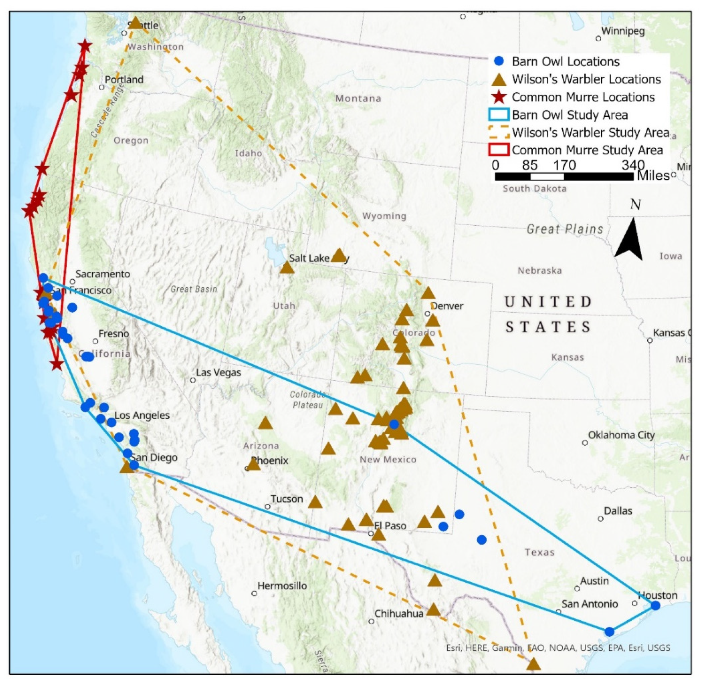
2.1. Citizen Science Avian Mortality Data and Study Area

We adopted the citizen science data of the three avian species with the highest reported death events from the southwest Avian Mortality Project under the iNaturalist platform: https://www.inaturalist.org/projects/southwest-avian-mortality-project (accessed on 20 December 2020). The quality grade of this dataset is “research-grade” and “Needs ID”. The data were collected from August–October 2020 by citizen scientists with each observation containing the photos, unique identity, genus, species, geographical locations, etc. There were 1357 avian mortality observations the study period involving 226 species during. Here, we focused on the three species that received the major impacts with the highest mortality observations, which are Wilson’s Warbler, Barn Owl, and Common Murre. There were 96, 40, and 33 mortality observations for Wilson’s Warbler, Barn Owl, and Common Murre, respectively (Figure 1). Each mortality event may represent multiple carcasses. However, considering the missing information on carcass counts in many observations, the difficulty in quantifying the numbers of carcasses in some photos, and the unknown species abundance, we focused on the occurrence of the mortality events for each species rather than the number of deaths. The study area for each species was defined as the minimum convex polygon of the observations with 10 km buffers (Figure 1) [32]. Additionally, it is also noteworthy that the New Mexico Department of Game & Fish [13] investigated most of the collected dead samples and found that those mortalities were not related to diseases.

2.2. Earth Observation Data

We considered 20 covariates from multiple remotely sensed and grid datasets to account for the potential effects from the two abrupt environmental changes in August–October 2020 (Table 1). For the effects of wildfires, we included distance to the closest wildfire events, wildfire densities, the average daily maximum smoke level, and toxic gases. Distance to the closest wildfires and wildfire densities were computed by using “Euclidean Distance” and “Kernel Density” tools, respectively, in ArcGIS Pro 2.9 (ESRI Inc., Redlands, CA, USA) based on the wildfire location data [33]. The wildfire location data were obtained from the National Interagency Fire Center and screened for the wildfire events that lasted over a week between August and October 2020. We averaged the daily maximum smoke data during the study period, which was downloaded from the National Oceanic and Atmospheric Administration (NOAA) Hazard Mapping System Fire and Smoke Product.
We also incorporated high-resolution imagery of a series of toxic gas concentrations, including CO, NO2, and SO2. In this study, we also calculated the averages of the daily concentration of toxic gases, including CO, NO2, and SO2, which were accessed from Sentinel-5P TROPOMI near-real-time (NRTI) Level-3 data. NO2, CO, and SO2 enter the atmosphere as a result of anthropogenic activities and natural processes. Those retrieval-assimilation modeling systems use the three-dimensional global TM5-MP chemistry transport model at a resolution of 1 × 1 degree as an essential element [34]. The tool of Harpconvert [35] was used to grid the Level-3 data of Sentinel-5P TROPOMI by using the bin_spatial operation. Moreover, the source data were filtered to remove pixels with QA values less than 75% for NO2 and 50% for CO and SO2. Sentinel-5P TROPOMO datasets were acquired and aggregated to study period in Google Earth Engine (GEE). The Sentinel-5P Near Real-Time products with 1.1 km × 1.1 km resolution are the relative high-resolution data sources that are currently used to observe and monitor NO2, CO, and other toxic gases and aerosols [36,37].
To consider the early winter storm, we accessed the daily maximum snow covers during August–October, 2020 from the Moderate Imaging Spectroradiometer (MODIS) snow product—the MOD10A1 V6 Snow Cover Daily Global 500 m product from GEE. Additionally, we included the climatic measurements, such as maximum temperature, precipitation, and humidity, assessed from the Gridded Surface Meteorological (gridMET) dataset from National Integrated Drought Information System (NIDIS) with a resolution of 1/24th degree using the “ClimateR” package via R v.4.1.1 [38].
We considered land cover types (2019 National Land Cover Dataset; NLCD) and tree canopy coverage, accessed via GEE, to account for habitat selection of different species. We reclassified NLCD into shrub, forest, developed, grass, agriculture, and water land cover types, following [14,33]. Since the Common Murre spend most of their time in the water, we also included ocean temperature within a 100-km buffer to consider the ocean temperature in their potential habitat range [39]. The buffer was selected based on the core home range size for common murres [40,41]. Ocean temperature at a depth of 0 m was acquired from Hybrid Coordinate Ocean Model (HYCOM) with spatial resolution of 0.08 degrees via GEE [42]. Moreover, since there could be more records of citizen science data in highly human populated areas or the areas that are more accessible to humans, we also included the population data and distance to roads from the US Census Bureau (2020). All raster grids were preprocessed and resampled to the spatial resolution of ~4.5 km × 4.5 km using GEE to ensure the resolution of all layers match up with the climatic variables (maximum resolution of the variables).

2.3. Ensemble Random Forest Model

An ensemble Random Forest (RF) modeling was employed to identify how environmental changes affect the spatial distributions of the mortality of Wilson’s Warbler, Barn Owl, and Common Murre. RF derived from classification and regression trees generates a combination of trees using randomly selected bootstrap samples of the internal training data which were used to build the model. The number of bootstrap samples equals the number of trees (ntrees) selected. Each node of a tree is split by randomly selected sampling predictors (mtry is the number of them), and then the best split is selected. Model errors are estimated by predicting on an internal testing set (out-of-bag sample, OOB), which are the observations that were not selected to construct trees, to validate the model. The predictions are then aggregated for each ensemble tree. Despite the integrated internal validation based on OOB data in the RF algorithm, external validation using the data completely withheld from the model is often adopted to assess model performance and predictive accuracy.
We first filtered the spatial locations of the mortality observations for each species using the ~4.5 km × 4.5 km grids (i.e., the spatial resolution of environmental layers) to avoid model overfitting [43]. For each species, we randomly generated 300, 130, and 110 pseudo-absence data within the study area of Wilson’s Warbler, Barn Owl, and Common Murre, respectively (Figure S1). Similar to how we filtered the presence data, those pseudo-absence data were also restricted to locate at least 4.5 km apart from each other. We then used three strategies with presence and pseudo-absence radio as 1:1, 1:2, and 1:3 to randomly draw the pseudo-absence data with replacement for RF model development. We used three strategies because the generation of pseudo-absence data might influence the results, and those ratios have been suggested in a pretty good performance in machine learning algorithms [44]. For each strategy, we generated 20 random draws (a total of 60).
We built separate RF models for each of the three species using “random forest” R-package in R v4.1.1 [38]. We employed an ensemble modeling approach to integrate information from 60 RF models that were developed using 60 sets of presence and pseudo-absence data for each species. For each RF model, we applied the common 80/20 random split for external training and testing sets. The external training sets were used to build RF models, while the external testing sets were used for model validation and performance estimation. To reduce the potential impacts of multicollinearity issues, we filtered the variables by testing Pearson’s coefficient (Figures S2–S4). For any pair of covariates with the absolute values of Pearson’s coefficient greater than 0.7 (|r| > 0.7), we included the one with high contributions in the model [45]. Then, variables with averaged contributions to the 60 models greater than 2% were included in the final ensemble models. We summarized he final combination of variables included in the RF models for each species in Table 2. For the development of RF models, since both theoretical and empirical research suggested that the classification accuracy is less sensitive to ntree than mtry [46,47], we tuned the mtry to identify the optimal parameters by controlling ntree = 500 (default and one of the common settings). The optimal set of parameters for each species, including mtry, nodesize (node size), and sampsize (number of sample to draw in strata), was identified using the “tuneRanger” R-package [48]. See the optimal set of parameters that we used to run the final models in Table S1. The 60 individual RF models for each species were finally combined into an ensemble prediction to capture the spatial distribution of potential mortality that could be found for Wilson’s Warbler, Barn Owl, and Common Murre in the western and central United States. Additionally, we also computed the uncertainty in model prediction by considering the 95% confidence intervals in predicted ensemble probabilities of mortality occurrence at each pixel [49]. To estimate the model performance, we calculated the Area Under the Receiver Operating Characteristic (ROC) Curve (AUC) for both external training and testing sets. Variable contributions in the RF models were assessed via partial dependence plots.

3. Results

3.1. Wilson’s Warbler’s Mortality

The ensemble RF modeling suggested that high-risk mortality corridors for Wilson’s Warbler were identified from north-central Colorado to north-central New Mexico (Figure 2). Other high probability areas included south-central New Mexico, western-central and southern California, and south-central Washington. Prediction uncertainty ranging from 0–0.30 was scaled to a range of 0–1, with the highest results surrounding north-central New Mexico and southern Texas. The RF modeling showed exceptional performance with a predictive accuracy (AUC) of 0.96 and 0.97 for external training and testing sets, respectively (Table 2). Since the data were collected by citizen scientists, the probability of observing a mortality event was higher in urban areas and close to roads compared to other regions (Figure 3). Additionally, more deaths were reported in areas with higher average daily maximum snow cover. Regarding the effects of wildfires, the probability of mortality events first decreased, then increased with the increasing intensity of fire density, CO, and SO2 concentration, as well as maximum smoke level.

3.2. Barn Owl’s Mortality

The ensemble RF models used to describe the spatial distributions of the Barn Owl had an overall good performance and predictive power with external training AUC of 0.95 and external testing AUC of 0.93 (Table 2). Mortality events were primarily predicted to occur in western California, despite the relatively high uncertainty (Figure 4). Similar to Wilson’s Warbler, we found the high probability of Barn Owl mortality events in urban areas with higher populations and closer to roads (Figure 5). Additionally, the probability of Barn Owl mortality first decreased and then increased with the increasing maximum smoke level and SO2 concentrations, which are two important variables influencing model accuracy. Additionally, more mortalities were detected in the areas with high level of snow covers.

3.3. Common Murre’s Mortality

The ensemble RF models with an AUC at 0.98 (Table 2) outputted the high probability of the mortality of the Common Murre at the coastline of central California and northern Oregon (Figure 6). Prediction uncertainty ranging from 0–0.20 was the highest in the southern corner of the study area. Daily maximum temperature, tree canopy, and precipitation are the three most influential variables in the models, showing the negative correlations (Figure 7). Regarding the potential effects of wildfires and wildfire-induced air pollution, we found that the Common Murre deaths were likely to be in areas with low wildfire density and low levels of air pollution (daily maximum smoke and NO2). The findings also suggested that the probability for observing Common Murre deaths surged to highest in areas where the surrounding seawater temperature was highest.

4. Discussion

Unprepared environmental changes, such as severe weathers and other natural hazards, can have a catastrophic impact on species by causing direct mortality, habitat loss and fragmentations, and loss of food resources. In August–October 2020, massive bird mortalities were observed by citizen scientists across the western and central United States, accompanied by two abrupt environmental changes, i.e., extensive wildfires and an early winter storm. Different species occupying different niches in ecosystems may respond to such environmental impacts in different ways. In this study, we focused on the top three avian species that have been recorded with the highest mortality in August–October 2020 and investigated the effects of wildfires and the winter storm on the spatial distributions of the mortality events among different species.
Our findings revealed that Wilson’s Warbler had the highest mean decrease in accuracy metric for snow cover (14.1%) in the ensemble RF modeling, compared to the other two species, suggesting that the Wilson’s Warbler responded more significantly to the snow cover than others. The mean decrease accuracy measures the importance of a variable in the RF models by estimating the changes in predictive accuracy between the randomly permuted values and the original observations of the variable [50]. Wilson’s Warbler mortality events were more likely found in areas with high average snow cover. It has been suggested that most insectivore songbirds were under poor or severely emaciated body conditions, with physical exertion which has no nourishment to support recovery [13]. Some malfunctions included kidney failure, empty stomach and intestines, fat deposits, and irritated lung tissues. Abnormally early winter storms could trigger bird migration instincts before they are physically ready. Snow cover also mildly contributed to the RF model accuracy of the Barn Owl (mean decrease in accuracy metric of 2.1%), but was not included in the final RF models for the Common Murre due to the low mean decrease in accuracy metric (<2%). Our findings also aligned with some previous studies, which indicated that the Barn Owl often inhabit areas with no extensive snow cover [51,52]. The Barn Owl is often particularly sensitive to winter-induced starvation due to long-term food deprivation in the cold. Therefore, the short-term winter storms might affect the Barn Owls population because of unpreparedness; however, it often has lower impacts than long, extreme winters.
Our modeling results indicated that Barn Owls reacted to wildfire-induced toxic gases more significantly than Wilson’s Warbler and the Common Murre. The average concentration of NO2, SO2, and average daily maximum smoke level were three of the most influential covariates in the ensemble RF models for Barn Owls, with a mean decrease in accuracy metrics at 30.9%, 24.5%, and 9.4%, respectively. Most likely, the Barn Owl mortality events were detected at areas with high air pollution. The average daily maximum smoke level was also detected as one of the important covariates in the RF models for Wilson’s Warbler but with negative correlations. Additionally, toxic gases were identified as the least influential factors for predicting the spatial distributions of Common Murre. Birds can be particularly vulnerable to air pollutants. Although New Mexico Department of Game & Fish (2020) [13] did not find biological evidence that mortalities of these avian species were primarily caused by wildfire-induced toxic gases, there still could be the potential of mild effects on bird health. The avian respiratory system is characterized by unidirectional airflow and cross-current gas exchanges to support more efficient respiration than most terrestrial animals [53]. Therefore, avian species are more vulnerable to high concentrations of air pollutants than other mammals [54]. Wildfires and wildfire-induced smoke can also negatively impact the food security of avian species by destroying habitats and reducing visibility, making foraging difficult.
We found more avian mortality events were recorded close to urban areas to the data acquisition process and population density. The avian mortality datasets were collected by citizen scientists, leading to potential difficulties in accessing areas close to wildfires. Additionally, we found that avian mortality events were more likely to occur close to urban areas with high population densities and easily accessible areas (i.e., close to roads), where citizen scientists were more likely to be present [55].
Yang et al. [14] explored the environmental drivers on the overall patterns of avian mortalities; however, the species-specific investigations in this study allowed consideration of the different biology and ecology of each bird species to disentangle and compare their differences in responses to abrupt environmental changes. Particularly, we found that the mortality of Common Murre may not be significantly related to neither wildfires nor winter storms. Their deaths may be more related to a large patch of anomalously warm water (i.e., surgency in mortality probability with high sea water temperature), which was also reported in [21] as the primary driver of mortality events of the Common Murre in 2015.
Our study also has several limitations. First, we only modeled the presence of mortality observations rather than the number of deaths. Thus, one observation might include multiple carcasses. This is due to the missing information on carcass counts in observations, the difficulty in quantifying the numbers of carcasses in some photos, and the unknown species abundance. Thus, the spatial prediction might not represent the severity of the events. Second, although the New Mexico Department of Game & Fish have examined most of the mortality samples and found those deaths were not related to diseases [13], there were still chances that some mortality events were natural deaths or related to causes other than what we included here (e.g., atmospheric effects such as lightning). Third, the quality of citizen science data has historically been concerned in academic research, since the data are often collected by non-professionals. However, there are some “superusers” who often make significant contributions to the mapping project or some amateurs can act as data quality filters to correct information collected by other contributors [56]. Additionally, many online platforms have employed a multiuser environmental validation process, indicating a possible “wiki” principle of data validation [57]. Finally, we controlled the ntree in the RF models. Although the impacts of different ntree to model output can low, different settings of ntree might still affect the prediction slightly.

5. Conclusions

Despite evidence that suggests potential determinations of the massive avian mortality outbreaks are associated with the abrupt environmental changes caused by natural hazards, the species-specific responses to such crises have not been explicitly understood. In this study, we investigated the responses of the three species (i.e., Wilson’s Warbler, Barn Owl, and Common Murre) with the highest reported mortality in the citizen science database to two abrupt environmental changes (wildfires and winter storms) using multiple remotely sensed and grid datasets and ensemble RF models. Our models performed relatively robust with AUC metrics > 0.9 for all three species. Our findings suggested that the mortality of Wilson’s Warbler was mainly determined by early winter storms, with more deaths identified in areas with high average maximum daily snow cover. Barn Owls responded to the effects of both environmental events but were most prominently impacted by the effects of wildfire-induced air pollution. Mortalities of the Common Murre may be more heavily influenced by increasing ocean water temperatures, rather than the effects of wildfires or winter storms. This study emphasized the importance of investigating the species-specific systems and their different responses to abrupt environmental changes, which could help understand the resilience of the avian community to unexpected environmental changes. This study also highlighted the application of remote sensing technology to large-scale conservation studies and natural hazards monitoring. Furthermore, the framework in this study that leveraged geo-tagged citizen science data, remotely sensed data, and machine learning algorithm can be employed to effectively understand other ecosystems patterns and processes.

Supplementary Materials

The following supporting information can be downloaded at: https://www.mdpi.com/article/10.3390/rs14102369/s1.

Author Contributions

A.Y. and D.Y. designed the study; M.R., A.Y. and D.Y. processed the data; A.Y. implemented the analyses and wrote the first draft of the manuscript. All authors contributed to manuscript writing and editing. All authors have read and agreed to the published version of the manuscript.

Funding

The computational resource of research is supported by Microsoft AI for Earth Microsoft Azure Compute Grant, no. 00010003601. MBR is funded by the Department of Geography and Environmental Sustainability at the University of Oklahoma.

Data Availability Statement

The research data of this study can be archived from Figshare at: https://doi.org/10.6084/m9.figshare.19184261.v1.

Conflicts of Interest

The authors declare no conflict of interest.

References

  1. Walther, G.-R.; Post, E.; Convey, P.; Menzel, A.; Parmesan, C.; Beebee, T.J.; Fromentin, J.-M.; Hoegh-Guldberg, O.; Bairlein, F. Ecological Responses to Recent Climate Change. Nature 2002, 416, 389–395. [Google Scholar] [CrossRef] [PubMed]
  2. Walther, G.-R. Community and Ecosystem Responses to Recent Climate Change. Philos. Trans. R. Soc. B Biol. Sci. 2010, 365, 2019–2024. [Google Scholar] [CrossRef] [PubMed]
  3. Hannah, L.; Flint, L.; Syphard, A.D.; Moritz, M.A.; Buckley, L.B.; McCullough, I.M. Fine-Grain Modeling of Species’ Response to Climate Change: Holdouts, Stepping-Stones, and Microrefugia. Trends Ecol. Evol. 2014, 29, 390–397. [Google Scholar] [CrossRef] [PubMed]
  4. Freeman, B.G.; Lee-Yaw, J.A.; Sunday, J.M.; Hargreaves, A.L. Expanding, Shifting and Shrinking: The Impact of Global Warming on Species’ Elevational Distributions. Glob. Ecol. Biogeogr. 2018, 27, 1268–1276. [Google Scholar] [CrossRef]
  5. Caula, S.; Marty, P.; Martin, J.-L. Seasonal Variation in Species Composition of an Urban Bird Community in Mediterranean France. Landsc. Urban Plan. 2008, 87, 1–9. [Google Scholar] [CrossRef]
  6. Jones, K.R.; Watson, J.E.; Possingham, H.P.; Klein, C.J. Incorporating Climate Change into Spatial Conservation Prioritisation: A Review. Biol. Conserv. 2016, 194, 121–130. [Google Scholar] [CrossRef] [Green Version]
  7. Seabrook, L.; McAlpine, C.; Baxter, G.; Rhodes, J.; Bradley, A.; Lunney, D. Drought-Driven Change in Wildlife Distribution and Numbers: A Case Study of Koalas in South West Queensland. Wildl. Res. 2011, 38, 509–524. [Google Scholar] [CrossRef]
  8. Lam, S.S.; Waugh, C.; Peng, W.; Sonne, C. Wildfire Puts Koalas at Risk of Extinction. Science 2020, 367, 750. [Google Scholar] [CrossRef]
  9. Boyle, W.A.; Norris, D.R.; Guglielmo, C.G. Storms Drive Altitudinal Migration in a Tropical Bird. Proc. R. Soc. B Biol. Sci. 2010, 277, 2511–2519. [Google Scholar] [CrossRef] [Green Version]
  10. Waide, R.B. Summary of the Response of Animal Populations to Hurricanes in the Caribbean. Biotropica 1991, 23, 508–512. [Google Scholar] [CrossRef]
  11. Johnson, K. The Southwest Is Facing an ‘Unprecedented’ Migratory Bird Die-Off. Audubon Mag. 2020. Available online: https://www.audubon.org/news/the-southwest-facing-unprecedented-migratory-bird-die (accessed on 21 September 2021).
  12. Insurance Information Institute Facts + Statistics: Wildfires 2020. Available online: https://www.iii.org/fact-statistic/facts-statistics-wildfires (accessed on 21 September 2021).
  13. New Mexico Department of Game & Fish Starvation. Unexpected Weather to Blame in Mass Migratory Songbird Mortality. 2020. Available online: https://www.wildlife.state.nm.us/starvation-unexpected-weather-to-blame-in-mass-migratory-songbird-mortality/ (accessed on 21 September 2021).
  14. Yang, D.; Yang, A.; Yang, J.; Xu, R.; Qiu, H. Unprecedented Migratory Bird Die-off: A Citizen-based Analysis on the Spatiotemporal Patterns of Mass Mortality Events in the Western United States. GeoHealth 2021, 5, e2021GH000395. [Google Scholar] [CrossRef] [PubMed]
  15. Ruiz-Sánchez, A.; Renton, K.; Landgrave-Ramírez, R.; Mora-Aguilar, E.F.; Rojas-Soto, O. Ecological Niche Variation in the Wilson’s Warbler Cardellina Pusilla Complex. J. Avian Biol. 2015, 46, 516–527. [Google Scholar] [CrossRef]
  16. Curson, J.; Quinn, D.; Beadle, D. Warblers of the Americas: An Identification Guide; Houghton Mifflin Harcourt: Boston, MA, USA, 1994; ISBN 0-395-70998-9. [Google Scholar]
  17. Dunn, J.L.; Garrett, K. A Field Guide to Warblers of North America; Houghton Mifflin Harcourt: Boston, MA, USA, 1997; Volume 49, ISBN 0-395-78321-6. [Google Scholar]
  18. Huang, A.C.; Elliott, J.E.; Cheng, K.M.; Ritland, K.; Ritland, C.E.; Thomsen, S.K.; Hindmarch, S.; Martin, K. Barn Owls (Tyto Alba) in Western North America: Phylogeographic Structure, Connectivity, and Genetic Diversity. Conserv. Genet. 2016, 17, 357–367. [Google Scholar] [CrossRef]
  19. Briggs, K.T.; Tyler, W.B.; Lewis, D.B.; Carlson, D.R. Bird Communities at Sea off California: 1975 to 1983; Cooper Ornithological Society Inc.: Lawrence, KS, USA, 1987; ISBN 0-935868-36-4. [Google Scholar]
  20. Roletto, J.; Mortenson, J.; Harrald, I.; Hall, J.; Grella, L. Beached Bird Surveys and Chronic Oil Pollution in Central California. Mar. Ornithol. 2003, 31, 21–28. [Google Scholar]
  21. Gibble, C.; Duerr, R.; Bodenstein, B.; Lindquist, K.; Lindsey, J.; Beck, J.; Henkel, L.; Roletto, J.; Harvey, J.; Kudela, R. Investigation of a Largescale Common Murre (Uria Aalge) Mortality Event in California, USA, in 2015. J. Wildl. Dis. 2018, 54, 569–574. [Google Scholar] [CrossRef]
  22. Ballatore, A.; Mooney, P. Conceptualising the Geographic World: The Dimensions of Negotiation in Crowdsourced Cartography. Int. J. Geogr. Inf. Sci. 2015, 29, 2310–2327. [Google Scholar] [CrossRef] [Green Version]
  23. Wang, K.; Franklin, S.E.; Guo, X.; Cattet, M. Remote Sensing of Ecology, Biodiversity and Conservation: A Review from the Perspective of Remote Sensing Specialists. Sensors 2010, 10, 9647–9667. [Google Scholar] [CrossRef]
  24. Pettorelli, N.; Safi, K.; Turner, W. Satellite Remote Sensing, Biodiversity Research and Conservation of the Future. Philos. Trans. R. Soc. B Biol. Sci. 2014, 369, 20130190. [Google Scholar] [CrossRef]
  25. Guanter, L.; Bacour, C.; Schneider, A.; Aben, I.; van Kempen, T.A.; Maignan, F.; Retscher, C.; Köhler, P.; Frankenberg, C.; Joiner, J. The TROPOSIF Global Sun-Induced Fluorescence Dataset from the Sentinel-5P TROPOMI Mission. Earth Syst. Sci. Data 2021, 13, 5423–5440. [Google Scholar] [CrossRef]
  26. Buchhorn, M.; Lesiv, M.; Tsendbazar, N.-E.; Herold, M.; Bertels, L.; Smets, B. Copernicus Global Land Cover Layers—Collection 2. Remote Sens. 2020, 12, 1044. [Google Scholar] [CrossRef] [Green Version]
  27. Vîrghileanu, M.; Săvulescu, I.; Mihai, B.-A.; Nistor, C.; Dobre, R. Nitrogen Dioxide (NO2) Pollution Monitoring with Sentinel-5P Satellite Imagery over Europe during the Coronavirus Pandemic Outbreak. Remote Sens. 2020, 12, 3575. [Google Scholar] [CrossRef]
  28. Bello, O.M.; Aina, Y.A. Satellite Remote Sensing as a Tool in Disaster Management and Sustainable Development: Towards a Synergistic Approach. Procedia-Soc. Behav. Sci. 2014, 120, 365–373. [Google Scholar] [CrossRef] [Green Version]
  29. Kampichler, C.; Wieland, R.; Calmé, S.; Weissenberger, H.; Arriaga-Weiss, S. Classification in Conservation Biology: A Comparison of Five Machine-Learning Methods. Ecol. Inform. 2010, 5, 441–450. [Google Scholar] [CrossRef]
  30. Breiman, L. Random Forests. Mach. Learn. 2001, 45, 5–32. [Google Scholar] [CrossRef] [Green Version]
  31. Kracalik, I.T.; Kenu, E.; Ayamdooh, E.N.; Allegye-Cudjoe, E.; Polkuu, P.N.; Frimpong, J.A.; Nyarko, K.M.; Bower, W.A.; Traxler, R.; Blackburn, J.K. Modeling the Environmental Suitability of Anthrax in Ghana and Estimating Populations at Risk: Implications for Vaccination and Control. PLoS Negl. Trop. Dis. 2017, 11, e0005885. [Google Scholar] [CrossRef]
  32. Burgman, M.A.; Fox, J.C. Bias in Species Range Estimates from Minimum Convex Polygons: Implications for Conservation and Options for Improved Planning; Cambridge University Press: Cambridge, UK, 2003; Volume 6, pp. 19–28. [Google Scholar]
  33. Yang, A.; Yang, J.; Di Yang, R.X.; He, Y.; Aragon, A.; Qiu, H. Human Mobility to Parks Under the COVID-19 Pandemic and Wildfire Seasons in the Western and Central United States. GeoHealth 2021, 5, e2021GH000494. [Google Scholar] [CrossRef]
  34. Geffen, V.; Boersma, K.F.; Eskes, H.; Sneep, M.; Linden, T.; Zara, M.; Pepijn Veefkind, J. S5p TROPOMI NO2 Slant Column Retrieval: Method, Stability, Uncertainties and Comparisons with OMI. Atmos. Meas. Tech. 2020, 13, 1315–1335. [Google Scholar] [CrossRef] [Green Version]
  35. Harpconvert. Available online: http://stcorp.github.io/harp/doc/html/harpconvert.html (accessed on 13 February 2021).
  36. Verhoelst, T.; Compernolle, S.; Pinardi, G.; Lambert, J.-C.; Eskes, H.J.; Eichmann, K.-U.; Fjæraa, A.M.; Granville, J.; Niemeijer, S.; Cede, A. Ground-Based Validation of the Copernicus Sentinel-5p TROPOMI NO 2 Measurements with the NDACC ZSL-DOAS, MAX-DOAS and Pandonia Global Networks. Atmos. Meas. Tech. 2021, 14, 481–510. [Google Scholar] [CrossRef]
  37. Levelt, P.F.; Stein Zweers, D.C.; Aben, I.; Bauwens, M.; Borsdorff, T.; De Smedt, I.; Eskes, H.J.; Lerot, C.; Loyola, D.G.; Romahn, F. Air Quality Impacts of COVID-19 Lockdown Measures Detected from Space Using High Spatial Resolution Observations of Multiple Trace Gases from Sentinel-5P/TROPOMI. Atmos. Chem. Phys. Discuss. 2021, 1–53. [Google Scholar] [CrossRef]
  38. R Core Team. R: A Language and Environment for Statistical Computing; R Foundation for Statistical Computing: Vienna, Austria, 2021. [Google Scholar]
  39. Buren, A.D.; Koen-Alonso, M.; Montevecchi, W.A. Linking Predator Diet and Prey Availability: Common Murres and Capelin in the Northwest Atlantic. Mar. Ecol. Prog. Ser. 2012, 445, 25–35. [Google Scholar] [CrossRef]
  40. McFarlane Tranquilla, L.A.; Montevecchi, W.A.; Fifield, D.A.; Hedd, A.; Gaston, A.J.; Robertson, G.J.; Phillips, R.A. Individual Winter Movement Strategies in Two Species of Murre (Uria Spp.) in the Northwest Atlantic. PLoS ONE 2014, 9, e90583. [Google Scholar] [CrossRef] [PubMed]
  41. McFarlane Tranquilla, L.; Montevecchi, W.; Hedd, A.; Regular, P.; Robertson, G.; Fifield, D.; Devillers, R. Ecological Segregation among Thick-Billed Murres (Uria Lomvia) and Common Murres (Uria Aalge) in the Northwest Atlantic Persists through the Nonbreeding Season. Can. J. Zool. 2015, 93, 447–460. [Google Scholar] [CrossRef]
  42. Cummings, J.A.; Smedstad, O.M. Variational Data Assimilation for the Global Ocean. In Data Assimilation for Atmospheric, Oceanic and Hydrologic Applications; Springer: Berlin/Heidelberg, Germany, 2013; Volume II, pp. 303–343. [Google Scholar]
  43. Yang, A.; Gomez, J.P.; Blackburn, J.K. Exploring Environmental Coverages of Species: A New Variable Contribution Estimation Methodology for Rulesets from the Genetic Algorithm for Rule-Set Prediction. PeerJ 2020, 8, e8968. [Google Scholar] [CrossRef] [PubMed]
  44. Barbet-Massin, M.; Jiguet, F.; Albert, C.H.; Thuiller, W. Selecting Pseudo-absences for Species Distribution Models: How, Where and How Many? Methods Ecol. Evol. 2012, 3, 327–338. [Google Scholar] [CrossRef]
  45. Yang, A.; Proffitt, K.M.; Asher, V.; Ryan, S.J.; Blackburn, J.K. Sex-Specific Elk Resource Selection during the Anthrax Risk Period. J. Wildl. Manag. 2021, 85, 145–155. [Google Scholar] [CrossRef]
  46. Kulkarni, V.Y.; Sinha, P.K. Pruning of Random Forest Classifiers: A Survey and Future Directions. In Proceedings of the 2012 International Conference on Data Science & Engineering (ICDSE), Cochin, India, 18–20 July 2012; Institute of Electrical and Electronics Engineers: Piscataway, NJ, USA, 2012; pp. 64–68. [Google Scholar]
  47. Ghosh, A.; Sharma, R.; Joshi, P. Random Forest Classification of Urban Landscape Using Landsat Archive and Ancillary Data: Combining Seasonal Maps with Decision Level Fusion. Appl. Geogr. 2014, 48, 31–41. [Google Scholar] [CrossRef]
  48. Probst, P.; Wright, M.N.; Boulesteix, A. Hyperparameters and Tuning Strategies for Random Forest. Wiley Interdiscip. Rev. Data Min. Knowl. Discov. 2019, 9, e1301. [Google Scholar] [CrossRef] [Green Version]
  49. Deribe, K.; Cano, J.; Newport, M.J.; Golding, N.; Pullan, R.L.; Sime, H.; Gebretsadik, A.; Assefa, A.; Kebede, A.; Hailu, A. Mapping and Modelling the Geographical Distribution and Environmental Limits of Podoconiosis in Ethiopia. PLoS Negl. Trop. Dis. 2015, 9, e0003946. [Google Scholar] [CrossRef]
  50. Louppe, G.; Wehenkel, L.; Sutera, A.; Geurts, P. Understanding Variable Importances in Forests of Randomized Trees. In Proceedings of the Advances in Neural Information Processing Systems, Stateline, NV, USA, 5–10 December 2013. [Google Scholar]
  51. Marti, C.D.; Wagner, P.W. Winter Mortality in Common Barn-Owls and Its Effect on Population Density and Reproduction. Condor 1985, 87, 111–115. [Google Scholar] [CrossRef] [Green Version]
  52. Handrich, Y.; Nicolas, L.; Maho, Y.L. Winter Starvation in Captive Common Barn-Owls: Physiological States and Reversible Limits. Auk 1993, 110, 458–469. [Google Scholar] [CrossRef]
  53. Sanderfoot, O.V.; Holloway, T. Air Pollution Impacts on Avian Species via Inhalation Exposure and Associated Outcomes. Environ. Res. Lett. 2017, 12, 083002. [Google Scholar] [CrossRef] [Green Version]
  54. Brown, R.E.; Brain, J.D.; Wang, N. The Avian Respiratory System: A Unique Model for Studies of Respiratory Toxicosis and for Monitoring Air Quality. Environ. Health Perspect. 1997, 105, 188–200. [Google Scholar] [CrossRef] [PubMed]
  55. Davis, A.; Taylor, C.E.; Martin, J.M. Are Pro-Ecological Values Enough? Determining the Drivers and Extent of Participation in Citizen Science Programs. Hum. Dimens. Wildl. 2019, 24, 501–514. [Google Scholar] [CrossRef]
  56. Yang, D.; Yang, A.; Qiu, H.; Zhou, Y.; Herrero, H.; Fu, C.-S.; Yu, Q.; Tang, J. A Citizen-Contributed GIS Approach for Evaluating the Impacts of Land Use on Hurricane-Harvey-Induced Flooding in Houston Area. Land 2019, 8, 25. [Google Scholar] [CrossRef] [Green Version]
  57. Ballatore, A.; Jokar Arsanjani, J. Placing Wikimapia: An Exploratory Analysis. Int. J. Geogr. Inf. Sci. 2019, 33, 1633–1650. [Google Scholar] [CrossRef]
Figure 1. Citizen science observations for the mortality of Wilson’s Warbler (triangle), Barn Owl (circle), and Common Murre (star) in the western and central United States in 2020. Each symbol may represent multiple carcasses.
Remotesensing 14 02369 g001
Figure 2. Spatial distributions of the predicted mortality events and the uncertainty in predictions for Wilson’s Warbler in the western and central United States in 2020.
Remotesensing 14 02369 g002
Figure 3. Partial dependency plots of covariates used in the RF model to estimate the spatial distribution of the mortality of Wilson’s Warbler. The gray shading area indicates the confidence intervals derived from the model iterations. We report the mean decrease accuracy for each of the variables in the parentheses.
Remotesensing 14 02369 g003
Figure 4. Spatial distributions of the predicted mortality events and the uncertainty in predictions for Barn Owl in the western and central United States in 2020.
Remotesensing 14 02369 g004
Figure 5. Partial dependency plots of covariates used in the RF model to estimate the spatial distribution of the mortality of the Barn Owl. The gray shading area indicates the confidence intervals derived from the model iterations. We report the mean decrease accuracy for each of the variables in the parentheses.
Remotesensing 14 02369 g005
Figure 6. Spatial distributions of the predicted mortality events and the uncertainty in predictions for Common Murre in the western and central United States in 2020.
Remotesensing 14 02369 g006
Figure 7. Partial dependency plots of covariates used in the RF model to estimate the spatial distribution of the mortality of the Common Murre. The gray shading area indicates the confidence intervals derived from the model iterations. We report the mean decrease accuracy for each of the variables in the parentheses.
Remotesensing 14 02369 g007
Table 1. The details and sources of the covariates that were considered to describe the potential effects on the spatial distributions of the mortality of the three species.
FactorsCovariates DescriptionsSources
Wildfire effectsDistance to wildfire (km)The distance to the closest wildfiresNational Interagency Fire Center
Wildfire density (km2)Density of wildfires
Maximum smokeThe average of the daily maximum smoke levelNOAA Hazard Mapping System Fire and Smoke Product
Carbon monoxide (CO) (mol/m2)Average of daily CO concentrationSentinel-5P TROPOMI near-real-time (NRTI) Level-3
Sulfur dioxide (SO2) (mol/m2)Average of daily SO2 concentration
Nitrogen dioxide (NO2) (mol/m2)Average of daily NO2 concentration
Winter stormSnow cover Percentage of daily maximum snow cover MOD10A1 V6 Snow Cover Daily Global 500 m
Climatic conditions that might reflect bothMaximum Temperature (Celsius)Average of daily maximum temperaturegridMET dataset via “ClimateR” package
Precipitation (mm)Average of daily precipitation
Humidity (kg/kg)Average of daily humidity
Burn IndexAverage of burn index
Wind (m/s)Average of daily wind speed
Evapotranspiration (mm)Average of daily evapotranspiration
HabitatForest, shrub, developed, agriculture, grass, and waterBinary indicator for forest, shrub, developed, agriculture, grass, and water land2019 National Land Cover Dataset a
Ocean temperature (Celsius)Average of the daily maximum ocean temperature within a buffer of 100 kmHybrid Coordinate Ocean Model
Tree canopy (%)Percentage of tree canopy coverageMulti-Resolution Land Characteristics (MRLC) Consortium
Anthropogenic effects on observationCounty populationPopulation of the county where the observation was reportedCensus Bureau
Distance to roads (km)Euclidean distance to primary and secondary roadsTIGER/Line Census Data
a Here, we assumed that there were not that many changes in land cover types between 2020 and 2019.
Table 2. Random forest model structure to describe the spatial distribution of the mortality of Wilson’s Warbler, Barn Owl, and Common Murre. For each model, we reported the AUC for external training and testing sets to assess model performance and predictive accuracy, respectively. We reported the 95 confidence intervals for the AUC values in parentheses.
SpeciesModel StructureExternal Training AUCExternal Testing AUC
Wilson’s WarblerMaximum temperature + Precipitation + Burn index + Distance to roads + Maximum smoke + CO + SO2 + Forest + Wind + Developed + County population + Snow cover + Shrub + Evapotranspiration + Humidity + Wildfire Density 0.96 (0.96, 0.97)0.97 (0.96, 0.98)
Barn OwlTree canopy + Precipitation + Distance to roads + Maximum smoke + SO2 + NO2 + Forest + Wind + Developed + County population + Snow cover0.95 (0.94, 0.95)0.93 (0.90, 0.95)
Common MurreMaximum temperature + Tree canopy + Precipitation + Burn index + Ocean temperature + Distance to roads + Wildfire density + Maximum smoke + SO2 + NO20.98 (0.97, 0.99)0.98 (0.97, 0.99)
Publisher’s Note: MDPI stays neutral with regard to jurisdictional claims in published maps and institutional affiliations.

