Abstract
During the oil extraction procedure, natural gases escape from wells, and the process of recuperating such gases requires important investments from oil and gas companies. That is why, most often, they favor burning them with flares. This practice, which is frequently employed by oil-producing companies, is a major cause of greenhouse gas emissions. Under growing demands from the World Bank and environmental defenders, many producer countries are devoted to decreasing gas flaring. For this reason, several researchers in the oil and gas industry, academia, and governments are working to propose new methods for estimating flared gas volumes, and among the most used techniques are those that exploit remote sensing data, particularly Visible Infrared Imaging Radiometer Suite (VIIRS) Nighttime Light (NTL) ones. Indeed, it is possible to extract, from such data, some physical parameters of flames produced by gas flares. In this investigation, a linear spectral unmixing-based approach, which addresses the spectral variability phenomenon, was designed to estimate accurate physical parameters from VIIRS NTL data. Then, these parameters are used to derive flared gas volumes through intercepting zero polynomial regression models that exploit in situ measurements. Experiments based on synthetic data were first conducted to validate the proposed linear spectral unmixing-based approach. Second, experiments based on real VIIRS NTL data covering the flare, named FIT-M8-101A-1U and located in the Berkine basin (Hassi Messaoud) in Algeria, were carried out. Then, the obtained flared gas volumes were compared with in situ measurements.
1. Introduction
Gas flaring is the controlled burning of excess and residual gases, usually performed in a flare [1]. It is a common practice used in oil and gas exploration, production and processing. Gas flaring is, above all, considered a safety solution [2,3]. It prevents dramatic accidents due to overpressure caused by over-supplies or emergency shutdowns. It can be used as a routine control process to manage certain emissions that might otherwise be vented into the atmosphere, such as in oil fields where the flared gas is associated with petroleum gas (a form of natural gas dissolved in oil).
Gas flaring is also one of the major regional and global energy and environmental challenges facing the world. Indeed, it has been a multi-billion dollar waste and a local/global energy/environmental problem for decades [4].
In 2020, the World Bank’s Partnership Global Gas Flaring Reduction (GGFR) reported that the open-pit torches burned approximately 142 Billion Cubic Meters (BCM) of gas [5]. According to the GGFR, Russia, Iraq, Iran, the United States, Algeria, Venezuela and Nigeria continue to occupy the top of the ranking of countries emitting gas flares for nine consecutive years. These countries produce 40% of the World’s oil each year and hold about two-thirds (65%) of the World’s gas flares [5].
In recent years, oil and gas companies have become more committed to the environment and are investing more in projects that reduce greenhouse gas emissions [6]. This would help to achieve the Zero Routine Flaring (ZRF) objective in 2030, which was launched in 2015 by the World Bank and the United Nations Secretary-General. To date, 80 governments and oil and gas companies have made the ZRF commitment, collectively accounting for about 60% of global flaring [7]. To achieve the ZRF objective, oil-producing countries need to properly obtain better data reliability and accuracy of flares to further improve investments and reduce flaring activities [8].
Flared gas volumes are regularly quantified around the world by GGRF. Among the methods used are those that exploit remote sensing data, collected by spaceborne infrared sensors, combined with in situ measurements. These methods are now commonly used to detect flares and estimate flared gas volumes through data collected by the National Aeronautics and Space Administration/National Oceanic and Atmospheric Administration (NASA/NOAA) Visible Infrared Imaging Radiometer Suite (VIIRS) sensor on board the Suomi National Polar-orbiting Partnership (Suomi NPP) satellite. Inspired by work on thermal anomaly detection to fight forest fires [9], these methods use VIIRS Nighttime Lights (NTL) data to detect the infrared radiation from heat emitted by flare flames. This allows the estimation of various physical parameters of the flare, including flared gas volumes [10,11,12].
Such a classical method ignores the spectral mixing phenomenon due to the very low spatial resolution of the considered data [13]. Indeed, such a spatial resolution leads to the presence of mixed pixels that contain more than one ground object. Hence, each observed pixel spectrum becomes a mixture of object spectra present in the considered observed pixel. Moreover, flared gas volumes are usually estimated by employing the global coefficient proposed by the CEDIGAZ organization, which is an international not-for-profit association for natural gas [14]. The considered coefficient may be unsuitable, not updated, as illustrated in [11], and may not consider some particular flaring events.
In this paper, a linear spectral unmixing (LSU)-based approach [13], which addresses the spectral variability phenomenon [15,16], is designed to estimate flare physical parameters from VIIRS NTL data. These parameters are then used to derive flared gas volumes by intercepting zero polynomial regression models that employ in situ measurements. Moreover, the proposed approach aims to improve the results provided by the classical literature method. This classical approach, which is based on the modeling of the Planck law curve [10,11,12], uses the observed flare flame spectra that are assumed to be mixed, as they are. However, the proposed unmixing-based approach provides purer spectra that will improve the estimation of flare flame physical parameters.
In this investigation, experiments based on synthetic data are first conducted to validate the designed linear spectral unmixing-based approach. Second, experiments based on real VIIRS NTL data covering the flare, named FIT-M8-101A-1U and located in the Berkine basin (Hassi Messaoud) in Algeria, are carried out. Then, the obtained flared gas volumes are compared with in situ measurements provided by the Algerian national company SONATRACH (in French SOciété NAtionale pour la recherche, la production, le Transport, la Transformation et la Commercialisation des Hydrocarbures), during the two years of 2020 and 2021.
The remainder of this paper is organized as follows. The considered study area is described in Section 2. The materials used and the proposed approach are presented in Section 3. In Section 4, the obtained experimental results are presented. In Section 5, the achieved results are discussed. Finally, Section 6 concludes the investigation.
2. Study Area
In this investigation, experiments using synthetic data are conducted to validate the proposed unmixing-based approach. Additionally, the flare with its in situ measured flared gas volumes, named FIT-M8-101A-1U, located at 31°00′53″N and 08°09′47″E (Figure 1) in the Berkine basin (Hassi Messaoud) in Algeria, is selected to perform experiments considering the designed unmixing-based method and using real VIIRS NTL remote sensing data.
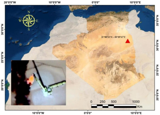
Figure 1.
The location of the considered gas flare FIT-M8-101A-1U in the Berkine basin (Hassi Messaoud) in Algeria.
It should be noted here that Algeria is the largest by area in African and Arab countries and the tenth in the world. Its economy is one of the most important in the region, showing indicators of rapid growth [17]. Moreover, Algeria, which contains significant natural resources, such as oil and gas, is an active member of the Organization of the Petroleum Exporting Countries (OPEC) and has great potential for economic and social development [18].
Furthermore, through the SONATRACH company, Algeria has several oil and gas flaring fields; among them, the five most significant are Alrar (Illizi), Hassi R’Mel, Tin Fouye Tabankort (TFT Illizi), Tiguentourine (In Amenas), and the considered Berkine basin in Hassi Messaoud [17]. This basin, with an area of 102,395 km2, is one of the oldest and largest oil fields in Algeria and the African continent [17]. It is located in the northeastern part of the Saharan Platform. It is limited to the West by the structural axes of Rhourde Nouss and to the South by the old mole of Ahara-El Ouar, of East–West orientation [17].
3. Materials and Methods
3.1. Used Data
As introduced, VIIRS NTL data were used in this investigation. It should be mentioned here that the multispectral VIIRS instrument, developed by the U.S. NASA, is one of the most used sensors for gas flaring detection and monitoring at both local and global scales. This instrument is on board the Suomi NPP and NOAA-20 satellites [19,20] and provides 22 spectral bands in the 0.4 to 12.6 μm spectral region [21,22]. In this work, the five NTL M-bands M7, M8, M10, M11 and M12 (Table 1) are the only ones used, with a spatial resolution of 750 m at nadir.

Table 1.
The used VIIRS NTL spectral bands covering the considered flare.
In addition, in situ measured flared gas volumes, during the two years 2020 and 2021 of the considered flare, provided by SONATRACH, are used in this work. More precisely, total “daily” measurements are provided and used for the two years 2020 and 2021, and “hourly” ones (the total between 01:00 and 02:00 UTC to get as close as possible to the remote sensing data acquisition time), of October and November 2021, are also provided and used in this investigation.
3.2. Estimation of Flare Physical Parameters
In this sub-section, some flare physical parameters and their estimation method, required for the proposed unmixing-based approach (detailed in the next sub-section), are described.
It should be highlighted that the considered VIIRS NTL spectral bands mainly record radiances from areas that contain heat sources, such as the nocturne lights of cities, fires or flare flames [21]. The other ground objects are considered background. Moreover, the recorded pixel spectrum with a higher value at spectral band M10 (see, for example, an illustration in Figure 2), as compared to those at M7, M8 and M12, indicates the presence of a flare (with a temperature between 1400 and 2000 Kelvin). The wavelength of the M10 band (Table 1) coincides with the peak of radiant emissions of gas flares and is located at one of the brightest atmospheric windows, ensuring a high degree of transmission from the flare flame to remote sensing sensors [21].
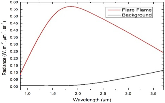
Figure 2.
An illustration of the flare flame and background spectra.
However, it should be noted that the very low spatial resolution of the used VIIRS NTL spectral bands leads to the presence of mixed pixels, which contain more than one ground object. Thus, it may be difficult to estimate flare physical parameters simply from such mixed pixels. Hence, a method based on the spectral unmixing concept is introduced in the next subsection. This proposed approach allows extraction of a pure (i.e., separated from the background) spectrum of flames and their area, of flares contained in a mixed pixel. This information is then used instead of the observed pixel spectrum and the complete footprint area of a pixel containing flare flames.
3.2.1. Flare Physical Parameters
The flare physical parameters estimation is based on Planck’s law, which describes the electromagnetic radiation emitted by a black body at the thermal equilibrium for a given temperature T (in Kelvin) according to [21]:
where the vector describes the spectral emissive power per unit area, per unit solid angle for a particular radiation wavelength, is the Planck constant (6.625 × 10⁻³⁴ J.s), is the light speed in the void (3 × 10⁸ m.s−1), , in micrometer, is a wavelength vector and is the Boltzmann constant (1.38 × 10⁻²³ J.K−1).
By considering, from VIIRS NTL data, the flame flare radiances in the considered spectral bands, it is then possible to model the Planck curves of gas flares. The temperature of the hot source is calculated using the Wien displacement law. This law is used to derive the temperature for a corresponding wavelength (in micrometer) of peak emission [21]:
3.2.2. Planck Curve Fitting
Responding to emissions at different wavelengths, observed flare flame spectra from the considered VIIRS NTL data allow a fitting to be performed by reproducing Planck curves and by varying two parameters, temperature and emissivity , which is defined as a maximum radiance ratio between a gray body and a black one (Figure 3).
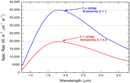
Figure 3.
An illustration of two Planck curves.
The two fitting outputs are estimates of the temperature and emissivity values of a flame (hot source) from a flare present in a given pixel of the considered VIIRS NTL data.
More specifically, the estimation is performed by applying a Planck curve fit on an observed flare flame spectrum obtained by the considered M7, M8, M10, M11 and M12 VIIRS NTL spectral bands, and this involves finding the Planck curve that best matches the manipulated flare flame spectrum.
3.2.3. Source Area Estimation
When considering the remote sensing data, in particular their spatial resolutions, a hot source, such as a flare flame, is contained in a sub-pixel; it only occupies a small portion of the pixel footprint on the ground. Therefore, the emissivity is first used as a scaling factor to estimate the area of that hot source. This area is estimated in square meters by multiplying by the estimated size of the pixel footprint size .
After that, the obtained is refined using a coefficient, which corresponds to the sub-pixel area occupied by a flare flame, estimated by the proposed unmixing-based approach introduced hereafter.
The pixel footprint size varies according to the zenith angle () of the sensor for a given flare location. Indeed, the considered VIIRS NTL data has a wide swath, and aggregation of pixels is used in 3 zones with different spatial resolutions [23].
This size is the product of VIIRS data along scan , and along track-pixel size (i.e., ). These are derived as follows:
where (radius of the Earth), (satellite nominal altitude), , , where (pixel size along scan), (pixel size along track). To address the three aggregation zones, the variable is designated as follows:
3.2.4. Radiant Heat Estimation
The flare temperature estimated after the Planck curve fitting and its size are used to calculate, by using the Stefan–Boltzmann law, the total hot source radiance or the Radiant Heat (or the power of the source in Mega Watt ()) as follows:
where is the Stefan–Boltzmann constant (5.67 × 10⁻⁸ J.K−4.m−2.s−1).
3.3. Proposed Spectral Unmixing Approach
3.3.1. Data Mixing Model
In this subsection, the considered mathematical data model is described. This is related to the well-known linear data mixing model used in the LSU field [13]. Indeed, when considering the used VIIRS NTL data, in particular their spatial resolutions, each observed pixel may contain a mixture of mainly two materials (called pure materials or endmembers in the spectral unmixing field [13]): a hot source (flare flame in this work) and background material. Thus, each observed pixel spectrum may be considered a mixture of flare flame and background spectra. The most considered mixing model is the linear one for its simplicity, and in such a configuration, each observed pixel spectrum becomes a linear mixture of flare flame and background spectra.
Thus, the nonnegative spectrum ( is the number of considered, in this work, VIIRS NTL spectral bands), associated with a pixel , is given by [13].
where the coefficients and , respectively, correspond to the nonnegative abundance fractions of the flare flame and background in the considered pixel (thus, as mentioned in (8), their sum is equal to one: this which is well-known as the sum-to-one constraint), and the vector (respectively,) corresponds to the nonnegative radiance spectrum of the flare flame (respectively, the background) contained, again, in the considered pixel [13].
Furthermore, since the temperature of a flare flame can be different from one flare to another, spectral variations in their spectra may result. These spectral variations, which describe the well-known spectral variability/intra-class variability phenomenon, must be considered in the linear data mixing model [15]. To address this phenomenon, model (8) is rewritten as follows [16]:
where the operator denotes the element-wise vector multiplication, (respectively, ) corresponds to the nonnegative variability coefficient vector for the version of a flare flame (respectively, a background) associated with the considered pixel . The vector (respectively,) is the nonnegative radiance spectrum of the flare flame (respectively, the background) that is considered a reference spectrum for the considered spectral variability phenomenon.
Furthermore, the nonnegative variability scale coefficients in the vectors and allow tuning the spectra and in each processed pixel with respect to the reference ones and . These vectors and are here constrained as follows
where and are fixed coefficient vectors controlling the minimum and maximum variability degrees [15]. Each coefficient of the vector (respectively,) is set to 0.8 (respectively, 1.2) in the conducted experiments (described hereafter).
3.3.2. Proposed Unmixing Algorithm
The proposed unmixing-based algorithm is inspired by those described in [15,16], which use a Nonnegative Matrix Factorization (NMF) [24] technique. Such an NMF technique is applied to whole data represented by variable matrices. However, this technique is adapted here for unmixing each considered pixel represented, this time, by variable vectors. Thus, the proposed approach aims to model the considered data using the linear mixing function defined by (9). The involved variables are , , and that respectively aim to estimate the coefficients and , and the vectors and . The designed algorithm minimizes the following cost function for a given pixel :
where represents the 2-norm.
The proposed unmixing-based algorithm, which deals with the spectral variability phenomenon, uses the following iterative and multiplicative update rules. These values provide nonnegative values for the considered variables when they are nonnegatively initialized (as described hereafter).
where the operator denotes the element-wise vector division, (.)T corresponds to the vector transpose and is a very small and positive value that is added to the denominator of each update rule to avoid division by zero. It should be noted that the estimated background variables and are not used later but are considered here to refine the estimation of the flare flame variables and . Moreover, the above-mentioned sum-to-one constraint of abundance fractions and , defined in (8) and (9), as well as the constraint defined by (10), are also considered at each iteration of the designed algorithm.
The designed algorithm, as standard NMF techniques, does not guarantee that it provides a unique solution. Its convergence point depends on its initialization. The reference spectra vectors and are estimated by the use of the Simplex Identification via Split Augmented Lagrangian (SISAL) [13] method applied to the whole considered data. Furthermore, each initial nonnegative non-zero value of and , which correspond to abundance fractions of flare flame and background materials, is set to or may be set using the Fully Constrained Least Squares (FCLS) [25] method. Additionally, each initial nonnegative non-zero value of and that correspond to variability scale coefficients is randomly set by considering the constraint defined by (10).
The optimization of all variables is stopped when the number of iterations reaches a predefined maximum value.
Once the optimization is done, the final pure flare flame spectrum associated with the considered pixel is calculated using the following expression:
The pure spectrum is then used to calculate more accurate temperature and emissivity values, noted here: and , of detected flared flames, in the considered pixel . Their estimated abundance fraction is also used to refine their surface in that pixel, noted here , as follows:
Therefore, the radiant heat, noted here , becomes
3.4. Flare Volume Estimation
There are many regression models used in the literature for the transition from radiant heat estimation to flared gas volumes, noted . The most commonly used model, such as the one proposed by CEDIGAZ [14], is the intercepting zero first-order polynomial regression model. It should be recalled here that this CEDIGAZ model is obtained by means of national data and in situ measurements collected annually from at least 47 countries [14]. This model, as introduced, may be unsuitable, not updated, as illustrated in [11], and not considering some particular flaring events in order to be used in the estimation, as reliably as possible, of flared gas volumes.
In this investigation, intercepting zero polynomial regression models are considered for the transition from the estimated , obtained from the considered VIIRS NTL data, to the flared gas volumes . This transition is achieved using the following expression:
where are the regression coefficients and is the degree of the considered intercepting zero polynomial regression.
3.5. Design of Experiments
3.5.1. Design of Experiments Based on Synthetic Data
Two sets of spectra (flare flame and background) from 0.865 to 3.700 μm, with spectral variability (Figure 4), are used to create 20 × 20-pixel synthetic data. The used background spectra are directly extracted from real VIIRS NTL data [18], while the flare flame spectra are obtained using Planck’s law Equation (1) by setting one of the two parameters, temperature or emissivity, for each created flare flame spectrum and varying the other.
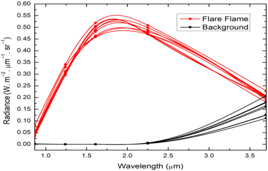
Figure 4.
The used sets of flare flame and background spectra, with spectral variability, used for creating synthetic data (flare flame spectra are obtained with 1550 Kelvin for the temperature and 1.5 × 10⁻⁵ for the emissivity).
The temperature parameter is thus set within an interval of standard values from 1500 to 1600 Kelvin with a step of 10, and the emissivity parameter is also set within an interval of standard values from 1.50 × 10⁻⁵ to 1.60 × 10⁻⁵ with a step of 10−7.
Thus, a set of 100 synthetic data are created from these spectra. Each pixel of these 100 images is obtained by linearly mixing spectra of the two considered materials (flare flame and background) after randomly selecting one spectrum for each material. Furthermore, from a land cover classification (Figure 5b) of a real RGB image of 2000 × 2000-pixel that covers a flare flame area (Figure 5a: the flare flame occupies, in this example, 37,488 pixels that represent 0.93% of the total image area) and abundance fraction maps (Figure 6) of 20 × 20-pixel used to create tested images are generated by averaging pixel classification values on a non-overlapping sliding window of 100 × 100-pixel. In addition, Gaussian noise is added to each generated synthetic image.
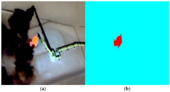
Figure 5.
(a) The considered real RGB data covering a flare area. (b) The corresponding two-class classification.
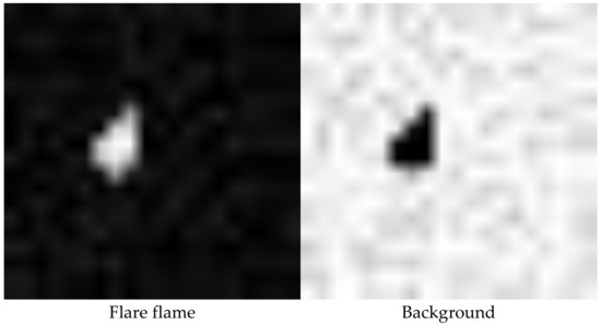
Figure 6.
The considered abundance fractions.
3.5.2. Design of Experiments Based on Real VIIRS NTL Data and In Situ Measured Flared Gas Volumes
When analyzing real data, 10 × 10-pixel data containing only the considered FIT-M8-101A-1U flare are used. These remote sensing data cover the two years of 2020 and 2021.
More specifically, remote sensing data for all April and May 2020 days (which represent the two most regular flaring months during 2020) are, first, used, with the provided “daily” in situ measured flared gas volumes, to establish an intercepting zero “first-order” polynomial regression model between estimated and provided in situ measurements. This model is used to estimate volumes by considering 156 days (spread over the whole 2020 year with 13 days per month (~3 days per week)). After that, the estimated volumes are compared to those measured and provided by SONATRACH.
Second, remote sensing data for all October and November 2021 days are considered, with the provided “hourly” (at 02:00 UTC in order to get as close as possible to the nocturnal time of remote sensing data acquisition) in situ measured flared gas volumes to set up an improved intercepting zero, this time, “third-order” polynomial regression model between estimated and provided in situ measurements. It should be mentioned here that October and November 2021 are chosen because they are the only months with “hourly” in situ measurements. The improved model, which allows the consideration of some particular flaring events, is then considered to estimate, by means of real VIIRS NTL data, more accurate volumes on the same above 156 dates of the year 2020.
In addition, the mean of estimated , during the two months of April and May 2020 (respectively, October and November 2021), is used to establish, by means of the proposed improved intercepting zero “third-order” polynomial regression model, an annual estimate, for 2020 (respectively, 2021), of flared gas volume by the considered FIT-M8-101A-1U flare. These estimated annual volumes are compared to those obtained by using the CEDIGAZ model and to those measured and provided by the SONATRACH.
3.6. Performance Evaluation Criteria
To evaluate the performance of the tested approaches, the following criteria are used: the Spectral Angle Mapper (SAM), the Normalized Mean Square Error (NMSE), the Root Mean Square Error (RMSE) and the determination coefficient . The SAM, NMSE and RMSE criteria are used when considering synthetic data, while the RMSE and criteria are used when considering real ones. These criteria read:
where is the original spectrum of the flare flame and is its estimate, denotes the vector norm, is the original value of the considered parameter of the flare and is its estimate, is the number of tests carried out that also corresponds to the number of generated synthetic data. As stated above, the RMSE criterion is also used when considering real data, and in that case is the value of the provided in situ measured flared gas volume, and is its estimate with the considered polynomial regression model; thus, becomes the number of in situ measures.
Smaller values of the SAM, NMSE and RMSE criteria indicate a better estimation, while for the determination coefficient , which ranges between 0 and 1 and evaluates the considered polynomial regression capacity in the description of the points distribution, a value close to 1 corresponds to strong predictive power.
4. Results
Obtained results, using synthetic data, are those achieved by applying the “classical” approach (i.e., the approach that does not use the spectral unmixing concept and only considers Equations (1)–(7)) and the designed unmixing-based one.
Furthermore, the obtained results, using real VIIRS NTL data combined with the provided in situ measured flared gas volumes, are also given. These ones are related to the flared gas volume estimations of the considered FIT-M8-101A-1U flare, using the established intercepting zero “first-order” (respectively, “third-order”) polynomial regression model when considering provided “daily” (respectively, “hourly”) in situ measurements.
Note here that the used performance evaluation criteria are only applied to the estimated parameter/volume values from the detected pixel of the tested synthetic and real VIIRS NTL remote sensing data, which contains the considered flare.
4.1. Obtained Results on Synthetic Data
Table 2 below shows the mean values of the considered SAM and NMSE performance criteria obtained by the tested approaches for the synthetic data, as well as the RMSE values of the estimated temperature and emissivity parameters.
Table 2.
Mean values of the SAM and NMSE criteria for the synthetic data and RMSE values of the estimated parameters (the bold values represent the best performances).
As an illustration, the following figure (Figure 7) shows the Planck curves identified after fitting with the spectra obtained with the tested approaches. Figure 8 then shows the original flare flame spectrum and its estimates, obtained with the tested approaches, from synthetic data generated with a temperature equal to 1550 Kelvin and an emissivity equal to 1.55 × 10⁻⁵.
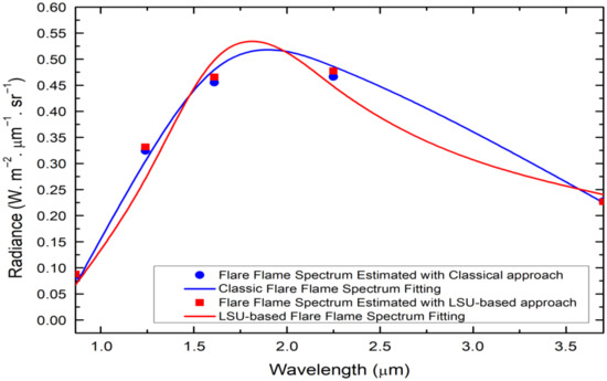
Figure 7.
Planck curve fits for a flare flame pixel and a flare flame pure spectra, estimated from synthetic data (with 1550 Kelvin for the temperature and 1.55 × 10⁻⁵ for the emissivity).
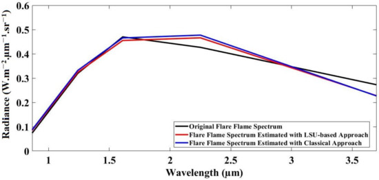
Figure 8.
Original flare flame spectrum and its estimates, obtained with the tested approaches, from synthetic data generated with a temperature = 1550 Kelvin and an emissivity = 1.55 × 10⁻⁵. Obtained values of the considered criteria for that case with the classical approach are SAM = 5.4502° and NMSE = 14.0294%, while these values with the designed unmixing-based approach are SAM = 2.3734° and NMSE = 12.1465%.
4.2. Obtained Results on Real VIIRS NTL Data Combined with Provided In Situ Measurements
Figure 9 shows the established intercepting zero “first-order” polynomial regression model, by using all April and May 2020 days, where are expressed in Mega Watts (MW) and the provided “daily” in situ flared gas volumes are expressed in Billion Cubic Meters (BCM).
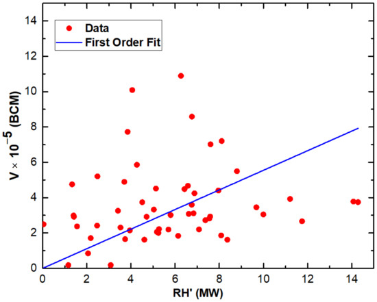
Figure 9.
The established intercepting zero “first-order” polynomial regression model, using all April and May 2020 days, by means of the proposed unmixing approach and the provided “daily” in situ flared gas volumes.
The obtained results (regression coefficients, determination coefficient, and RMSE values) by means of the established intercepting zero “firs-order” polynomial regression model, using all April and May 2020 days, are reported in the following table (Table 3).
Table 3.
Obtained results by means of the established intercepting zero “first-order” polynomial regression model using the two months of April and May 2020.
The next table (Table 4) reports the estimated annual 2020 flared gas volumes (in BCM) for the considered FIT-M8-101A-1U flare, obtained by means of the established intercepting zero “first-order” polynomial regression model using the two months of April and May 2020, and also by using the CEDIGAZ regression coefficient [14]. This table also reports the estimation errors (the absolute value of differences) between estimated flared gas volumes and measured ones by the SONATRACH.
Table 4.
Estimated annual 2020 flared gas volumes (in BCM) for the considered FIT-M8-101A-1U flare (the bold value represents the best estimation error).
The following figure (Figure 10) shows the established intercepting zero “third-order” polynomial regression model, by using all October and November 2021 days, where are expressed in MW and the provided “hourly” in situ measured flared gas volumes are expressed in BCM.
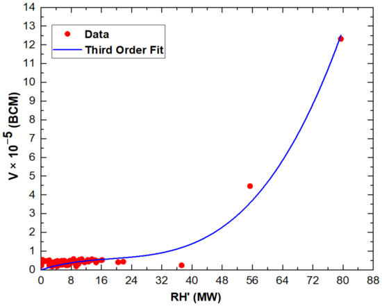
Figure 10.
The established intercepting zero “third-order” polynomial regression model, using all October and November 2021 days, by means of the proposed unmixing approach and the provided “hourly” in situ measured flared gas volumes.
The results obtained by means of the established intercepting zero “third-order” polynomial regression model, using all October and November 2021 days and considering the proposed unmixing-based approach, are reported in the following table (Table 5).
Table 5.
Obtained results by means of the established intercepting a zero “third-order” polynomial regression model using the two months of October and November 2021.
In addition, as an illustration in the next figure (Figure 11), values of “daily” (October and November 2021) flared gas volumes, provided by SONATRACH and those estimated by the proposed unmixing approach combined with the used “third-order” intercepting zero polynomial regression model applied on the provided “hourly” (at 02:00 UTC for October and November 2021) in situ measurements, are reported.
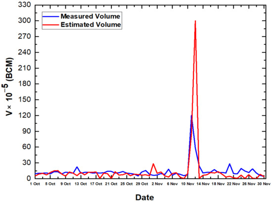
Figure 11.
Values of “daily” (October and November 2021) flared gas volumes, provided by the SONATRACH and those estimated by the proposed unmixing-approach combined with the used “third-order” regression model applied on the provided “hourly” in situ measurements.
The following table (Table 6) shows the estimated annual 2021 flared gas volumes (in BCM), for the considered FIT-M8-101A-1U flare, obtained by means of the established intercepting zero “third-order” polynomial regression model using the two months of October and November 2021, and also by using the CEDIGAZ regression coefficient [14]. Moreover, this table also reports the estimation errors (the absolute value of differences) between estimated flared gas volumes and measured ones by SONATRACH.
Table 6.
Estimated annual 2021 flared gas volumes (in BCM) for the considered FIT-M8-101A-1U flare (the bold value represents the best estimation error).
5. Discussion
When considering the tested realistic synthetic VIIRS NTL data, Table 2 shows that the proposed unmixing-based approach achieves better performance in terms of the estimation of flare parameters (temperature and emissivity) than the tested classical approach. This table shows that the designed unmixing-based approach provides the best SAM and NMSE values: the mean value of the SAM criterion obtained with the proposed unmixing-based approach is equal to 4.7263°, whereas the classical approach reaches a mean value equal to 6.9487°. In addition, for the NMSE criterion, the proposed unmixing-based approach achieves a mean value equal to 26.1295%, while the classical method reaches a mean value equal to 41.3251%.
Furthermore, from Figure 7, it can be seen that a spectrum resulting from the considered synthetic VIIRS NTL data for a pixel containing a flare flame, with the higher value in the spectral band M10, has lower amplitudes than the pure flare flame spectrum extracted by the considered unmixing-based approach in the same pixel. Indeed, given that the considered NTL data are characterized by a very low spatial resolution, the observed pixel spectrum is therefore a mixture of background and flare flame objects. Consequently, and since the mixture is assumed to be linear in the designed unmixing-based technique, the observed flare flame pixel spectrum (which also contains a larger area of background than the area occupied by the flare flame), used as in the classical approach, has lower amplitudes. As a result, when considering the proposed unmixing-based approach (with the pure flare flame spectrum), the Planck curve identified after fitting will have relatively higher amplitudes than those identified with the classical approach (with the mixed pixel spectrum).
Moreover, Figure 8 shows that the designed unmixing-based approach, unlike the tested classical approach, better extracts the flare flame spectrum, particularly in the spectral bands M7, M8 and M10.
The above results, obtained by means of synthetic data, motivated the adoption of the designed unmixing-based approach for its use on real VIIRS NTL data to estimate flared gas volumes by the considered FIT-M8-101A-1U flare.
When considering real VIIRS NTL data combined with those provided by SONATRACH, in situ flared gas volumes, Figure 9 and Figure 10, and Table 3, Table 4, Table 5 and Table 6 show the overall superiority in terms of flared gas volumes estimation of the proposed approach in comparison with the use of the CEDIGAZ regression coefficient.
In fact, Figure 9 and Table 3 report an acceptable determination coefficient, of the established, by using “daily” in situ measurements of the two months of April and May 2020, intercepting zero “first-order” polynomial regression model, with satisfactory RMSE results. Besides, a dispersion of points, in Figure 9, can be observed, and this is probably due to the fact that here the in situ volume measurements are “daily”, while the remote sensing estimations are almost instantaneous at about 02:00 UTC. Therefore, it is possible that particular flaring events (triggering procedures) occur at a time of day and are unobservable by the considered remote sensing data. Furthermore, Table 4 shows, for the considered FIT-M8-101A-1U flare, an annual 2020 flared gas volume estimation of 49.9559 × 10⁻³ BCM by means of the proposed approach, while this estimation is of 178.4253 × 10⁻³ BCM by using the CEDIGAZ regression coefficient. When considering the annual in situ measured flared gas volume provided by SONATRACH, which is of 66.6170 × 10⁻³ BCM, the absolute value estimation error of the proposed approach is equal to 16.6611 × 10⁻³ BCM, whereas this error is equal to 111.8083 × 10⁻³ BCM when using the CEDIGAZ regression coefficient. These results confirm the overall superiority of the designed approach.
On the other hand, Figure 10 and Table 5 show a good and improved determination coefficient of the established by means of “hourly” in situ measurements of the two months of October and November 2021, intercepting zero “third-order” polynomial regression model, with satisfactory and improved RMSE results. In particular, when considering the 156 dates of 2020, the RMSE value changes from 5.6935 × 10⁻⁵ BCM (Table 3), with the use of the intercepting zero “first-order” polynomial regression model and with provided “daily” in situ measurements of the two months of April and May 2020, to 5.2423 × 10⁻⁵ BCM (Table 5) with the use of the intercepting zero “third-order” polynomial regression model and with provided “hourly” in situ measurements of the two months of October and November 2021.
Additionally, Figure 11 shows a satisfactory consistency between “daily” (October and November 2021) values of measured and estimated flared gas volumes, by means of the proposed unmixing-based approach combined with the intercepting zero “third-order” polynomial regression model applied to the “hourly” (at 02:00 UTC) in situ measurements. More specifically, as shown in this figure (more precisely, as shown on 10–14 November 2021), the used “third-order” regression can, more or less, model certain particular flaring events that have occurred between 01:00 and 02:00 UTC, which are not always observable by considered remote sensing data if they occur at a time outside the acquisition time of these data. Hence, the interest in using “hourly” in situ measurements in accordance with the remote sensing data acquisition time (i.e., at 02:00 UTC for the considered VIIRS NTL data).
In this second configuration (i.e., the use of the intercepting zero “third-order” polynomial regression model and with provided “hourly” in situ measurements of the two months of October and November 2021), Table 6 reports, for the considered FIT-M8-101A-1U flare, an annual 2021 flared gas volume estimation of 33.0743 × 10⁻³ BCM by means of the proposed approach, while this estimation is 255.3538 × 10⁻³ BCM by using the CEDIGAZ regression coefficient. In comparison with the in situ measured volume provided by SONATRACH for the same year (i.e., 2021), which is of 67.6293 × 10⁻³ BCM, the absolute value estimation error of the proposed approach is equal to 34.5550 × 10⁻³ BCM, whereas this error is equal to 187.7245 × 10⁻³ BCM when utilizing the CEDIGAZ regression coefficient. These results again confirm the overall superiority of the designed approach.
Furthermore, estimation errors are always observed between calculated, using the proposed linear unmixing-based approach, and measured flared gas volumes. Such estimation errors may be reduced by considering in future works, more complex mixing models, such as nonlinear ones, and/or by using other non-polynomial regression models. Additionally, in the case of new estimates from new flares, the designed estimation models are to be updated by adding new flared gas volume estimations and measurements to old ones.
6. Conclusions
In this paper, an unmixing-based approach based on the linear spectral mixing model, which addresses the spectral variability phenomenon and uses a vector-based matrix factorization technique with nonnegativity constraints, is proposed for estimating flared gas volumes from VIIRS NTL remote sensing data. This designed approach consists of deriving pure flare flame spectra and its abundance fraction from considered remote sensing data that are then employed by physical law equations to estimate flare physical parameters.
Experiments based on synthetic data and real VIIRS NTL remote sensing images, as well as in situ flared gas volumes provided by SONATRACH, are conducted. First, synthetic data are considered to evaluate the performance, in terms of flare physical parameter estimation, of the designed unmixing-based approach. Consequently, the designed unmixing-based approach is applied to real VIIRS NTL data, which cover the FIT-M8-101A-1U flare (located at the Berkine basin, Hassi Messaoud, Algeria), by also considering the provided daily and hourly in situ flared gas volumes to estimate flared gas volumes during 2020 and 2021.
The obtained results show the overall superiority of the designed unmixing-based approach combined with intercepting zero polynomial regression models in terms of flared gas volume estimations compared with estimations achieved by using the CEDIGAZ regression coefficient.
An attractive extension of this investigation may consist of employing the designed unmixing-based approach on the whole Algerian territory to estimate global Algerian flared gas volumes.
Author Contributions
Conceptualization, F.Z.B. and M.S.K.; methodology, F.Z.B. and M.S.K.; software, F.Z.B. and M.S.K.; validation, F.Z.B., F.B., M.A.B. and M.S.K.; formal analysis, F.Z.B., F.B., M.A.B. and M.S.K.; investigation, F.Z.B., F.B., M.A.B. and M.S.K.; resources, F.Z.B., F.B., M.A.B. and M.S.K.; data curation, F.B. and M.A.B.; writing—original draft preparation, F.Z.B., F.B. and M.A.B.; writing—review and editing, M.S.K.; visualization, F.Z.B., F.B., M.A.B. and M.S.K.; supervision, M.S.K.; project administration, M.S.K.; funding acquisition, M.S.K. All authors have read and agreed to the published version of the manuscript.
Funding
This research received no external funding.
Acknowledgments
The authors would like to highly thank Fethi Benhamouda from the Agence Spatiale Algérienne (Alger, Algeria) for his support in carrying out these investigations. Additionally, the authors would like to greatly thank SONATRACH for providing daily and hourly in situ flaring gas volume measurements and for its support in conducting this work. Furthermore, the authors acknowledge the large NASA and NOAA efforts that provide publicly available VIIRS NtL remote sensing data.
Conflicts of Interest
The authors declare no conflict of interest.
References
- Emam, E.A. Gas Flaring in Industry: An Overview. Pet. Coal 2015, 57, 532–555. [Google Scholar]
- Torres, V.M.; Herndon, S.; Allen, D.T. Industrial Flare Performance at Low Flow Conditions. 2. Steam- and Air-Assisted Flares. Ind. Eng. Chem. Res. 2012, 51, 12569–12576. [Google Scholar] [CrossRef]
- Cheremisinoff, N.P. Industrial Gas Flaring Practices; John Wiley and Sons: Hoboken, NJ, USA, 2013; ISBN 978-1-118-67124-5. [Google Scholar]
- Ismail, O.S.; Umukoro, G.E. Global Impact of Gas Flaring. Energy Power Eng. 2012, 4, 290–302. [Google Scholar] [CrossRef] [Green Version]
- Global Gas Flaring Tracker Report. Available online: https://www.worldbank.org/en/topic/extractiveindustries/publication/global-gas-flaring-tracker-report (accessed on 3 March 2022).
- Mansoor, R.; Tahir, M. Recent Developments in Natural Gas Flaring Reduction and Reformation to Energy-Efficient Fuels: A Review. Energy Fuels 2021, 35, 3675–3714. [Google Scholar] [CrossRef]
- Zero Routine Flaring by 2030. Available online: https://www.worldbank.org/en/programs/zero-routine-flaring-by-2030 (accessed on 3 March 2022).
- Schade, G.W. Standardized Reporting Needed to Improve Accuracy of Flaring Data. Energies 2021, 14, 6575. [Google Scholar] [CrossRef]
- Hua, L.; Shao, G. The Progress of Operational Forest Fire Monitoring with Infrared Remote Sensing. J. For. Res. 2017, 28, 215–229. [Google Scholar] [CrossRef]
- Elvidge, C.D.; Bazilian, M.D.; Zhizhin, M.; Ghosh, T.; Baugh, K.; Hsu, F.-C. The Potential Role of Natural Gas Flaring in Meeting Greenhouse Gas Mitigation Targets. Energy Strategy Rev. 2018, 20, 156–162. [Google Scholar] [CrossRef]
- Zhizhin, M.; Matveev, A.; Ghosh, T.; Hsu, F.-C.; Howells, M.; Elvidge, C. Measuring Gas Flaring in Russia with Multispectral VIIRS Nightfire. Remote Sens. 2021, 13, 3078. [Google Scholar] [CrossRef]
- Elvidge, C.; Zhizhin, M.; Baugh, K.; Hsu, F.-C.; Ghosh, T. Methods for Global Survey of Natural Gas Flaring from Visible Infrared Imaging Radiometer Suite Data. Energies 2015, 9, 14. [Google Scholar] [CrossRef]
- Bioucas-Dias, J.M.; Plaza, A.; Dobigeon, N.; Parente, M.; Du, Q.; Gader, P.; Chanussot, J. Hyperspectral Unmixing Overview: Geometrical, Statistical, and Sparse Regression-Based Approaches. IEEE J. Sel. Top. Appl. Earth Obs. Remote Sens. 2012, 5, 354–379. [Google Scholar] [CrossRef] [Green Version]
- Cedigaz. Available online: https://www.cedigaz.org (accessed on 3 March 2022).
- Revel, C.; Deville, Y.; Achard, V.; Briottet, X.; Weber, C. Inertia-Constrained Pixel-by-Pixel Nonnegative Matrix Factorisation: A Hyperspectral Unmixing Method Dealing with Intra-Class Variability. Remote Sens. 2018, 10, 1706. [Google Scholar] [CrossRef] [Green Version]
- Benhalouche, F.Z.; Karoui, M.S.; Deville, Y. An NMF-Based Approach for Hyperspectral Unmixing Using a New Multiplicative-Tuning Linear Mixing Model to Address Spectral Variability. In Proceedings of the 27th European Signal Processing Conference (EUSIPCO), A Coruna, Spain, 2–6 September 2019; pp. 1–5. [Google Scholar] [CrossRef]
- Available online: https://www.energy.gov.dz/?Rubrique=hydrocarbure (accessed on 3 March 2022).
- OPEC. Available online: https://www.opec.org/opec_web/En/index.htm (accessed on 3 March 2022).
- Cao, C.; Xiong, X.J.; Wolfe, R.; DeLuccia, F.; Liu, Q.M.; Blonski, S.; Lin, G.G.; Nishihama, M.; Pogorzala, D.; Oudrari, H.; et al. Visible Infrared Imaging Radiometer Suite (VIIRS) Sensor Data Record (SDR) User’s Guide; NOAA Technical Report NESDIS: College Park, MD, USA, 2017. [Google Scholar]
- Miller, S.; Straka, W.; Mills, S.; Elvidge, C.; Lee, T.; Solbrig, J.; Walther, A.; Heidinger, A.; Weiss, S. Illuminating the Capabilities of the Suomi National Polar-Orbiting Partnership (NPP) Visible Infrared Imaging Radiometer Suite (VIIRS) Day/Night Band. Remote Sens. 2013, 5, 6717–6766. [Google Scholar] [CrossRef] [Green Version]
- Elvidge, C.; Zhizhin, M.; Hsu, F.-C.; Baugh, K. VIIRS Nightfire: Satellite Pyrometry at Night. Remote Sens. 2013, 5, 4423–4449. [Google Scholar] [CrossRef] [Green Version]
- Hillger, D.; Kopp, T.; Lee, T.; Lindsey, D.; Seaman, C.; Miller, S.; Solbrig, J.; Kidder, S.; Bachmeier, S.; Jasmin, T.; et al. First-Light Imagery from SUOMI NPP VIIRS. Bull. Am. Meteorol. Soc. 2013, 94, 1019–1029. [Google Scholar] [CrossRef]
- Polivka, T.N.; Hyer, E.J.; Wang, J.; Peterson, D.A. First Global Analysis of Saturation Artifacts in the VIIRS Infrared Channels and the Effects of Sample Aggregation. IEEE Geosci. Remote Sens. Lett. 2015, 12, 1262–1266. [Google Scholar] [CrossRef]
- Cichocki, A.; Zdunek, R.; Phan, A.H.; Amari, S. Nonnegative Matrix and Tensor Factorizations: Applications to Exploratory Multi-Way Data Analysis and Blind Source Separation; John Wiley and Sons: Hoboken, NJ, USA, 2009; ISBN 978-0-470-74728-5. [Google Scholar]
- Heinz, D.C.; Chang, C.-I. Fully Constrained Least Squares Linear Spectral Mixture Analysis Method for Material Quantification in Hyperspectral Imagery. IEEE Trans. Geosci. Remote Sens. 2001, 39, 529–545. [Google Scholar] [CrossRef] [Green Version]
Publisher’s Note: MDPI stays neutral with regard to jurisdictional claims in published maps and institutional affiliations. |
© 2022 by the authors. Licensee MDPI, Basel, Switzerland. This article is an open access article distributed under the terms and conditions of the Creative Commons Attribution (CC BY) license (https://creativecommons.org/licenses/by/4.0/).