Article

Cross-Sensor Nighttime Lights Image Calibration for DMSP/OLS and SNPP/VIIRS with Residual U-Net

1
Moscow Institute of Physics and Technology, 117303 Moscow, Russia
2
Earth Observation Group, Payne Institute, Colorado School of Mines, Golden, CO 80401, USA
3
Space Research Institute, Russian Academy of Sciences, 117997 Moscow, Russia
4
NRC “Kurchatov Institute”, 123182 Moscow, Russia
*
Author to whom correspondence should be addressed.
Remote Sens. 2021, 13(24), 5026; https://doi.org/10.3390/rs13245026
Submission received: 7 September 2021 / Revised: 3 November 2021 / Accepted: 6 December 2021 / Published: 10 December 2021
(This article belongs to the Special Issue Artificial Intelligence in Nighttime Remote Sensing)

Abstract

:
Remote sensing of nighttime lights (NTL) is widely used in socio-economic studies of economic growth, urbanization, stability of power grid, environmental light pollution, pandemics and military conflicts. Currently, NTL data are collected with two sensors: (1) Operational Line-scan System (OLS) onboard the satellites from the Defense Meteorology Satellite Program (DMSP) and (2) Visible Infrared Imaging Radiometer Suite (VIIRS) onboard the Suomi NPP (SNPP) and NOAA-20 satellites from the Joint Polar Satellite System (JPSS). However, the nighttime images acquired by these two sensors are incompatible in spatial resolution and dynamic range. To address this problem, we propose a method for the cross-sensor calibration with residual U-net convolutional neural network (CNN). The CNN produces DMSP-like NTL composites from the VIIRS annual NTL composites. The pixel radiances predicted from VIIRS are highly correlated with NTL observed with OLS (0.96 < R2 < 0.99). The method can be used to extend long-term series of annual NTL after the end of DMSP mission or to cross-calibrate same year NTL from different satellites to study diurnal variations.

1. Introduction

Defense Meteorology Satellite Program (DMSP) was launched in 1962 and since then its satellites with Operational Line-scan System (OLS) serve as a source of valuable night-time light (NTL) data of the Earth surface. Starting from 1992 the DMSP satellites broadcast digital images, which were post-processed by the NOAA (currently Colorado School of Mines) Earth Observation Group (EOG) into global annual average and background removed NTL maps. With annual data stretch from 1992 to 2013, it makes DMSP Nighttime Lights the longest data series available for nocturnal remote sensing on human activities [1]. In 2011 Suomi NPP (SNPP) satellite with Visible Infrared Imaging Radiometer Suite (VIIRS) was launched. VIIRS instrument is also capable of detecting dim light sources at night. Annual VIIRS maps of nighttime lights are published from 2013 to 2019 [2]. NTL maps made with DMSP (DNL) or VIIRS (VNL) are widely utilized in research of human activity, economy and ecology [3].
Despite the value of the long-term archives from DMSP and VIIRS, their potential is not fully utilized. The main reason is that there is a significant difference between the OLS and VIIRS sensors (Table 1). VIIRS is significantly superior to OLS in terms of spatial, temporal, and radiometric resolution [4]. Due to the lack of calibration, DMSP data have no radiometric measurement units whilst VIIRS output is measured in nW/cm2/sr. DMSP-OLS and VIIRS sensors differ significantly in terms of dynamic range: data from DMSP is quantized with 6-bit discrete values, i.e., the image values range from 0 to 63, whereas VIIRS DNB has a much wider dynamic range, the maximum values reach about 105 nW/cm2/sr [5]. Another negative effect present in the DMSP-OLS images is the sensor saturation in bright regions like city centers or gas flares, but there is no such effect in VIIRS images. All that makes the data from VIIRS and DMSP sensors difficult to cross-calibrate and jointly use in the NTL change studies.
Additionally, two satellite generations have different overpass times and thus they observe slightly different states of the city lights. The original DMSP annual NTL composites were produced using OLS data from six individual satellites F10, F12, F14, F15, F16 and F18. Over time, the orbits of each DMSP satellite gradually shift to an earlier overpass time, sliding from a day/night orbit to a dawn/dusk orbit. The OLS sensors collect sufficient nighttime data worldwide for annual NTL product generation as long as the overpass occurred later than 19:30. Recently, EOG has added additional years to the DMSP equatorial crossing time chart and discovered (Figure 1) that the F15 satellite orbit had continued to shift and had started to collect pre-dawn nighttime data in 2012 and it continues through 2020. Satellite F16 has also collected usable nighttime data in the pre-dawn hours. Based on this new information, EOG has extended the time series of the annual DNL maps out to 2019 using pre-dawn data from F15 and F16.
Due to the lack of methods for cross-sensor image calibration from different generations of satellites, almost all NTL-related research in sociology, economy or ecology was limited to data from either DMSP or VIIRS [3]. Several attempts were made to cross-calibrate the NTL products from all the DMSP satellites [6] as well as both VIIRS and DMSP sensors [7,8,9]. They utilize different approaches like Pseudo-Invariant Feature paradigm (PIF) or Regression Models. The problem with most of these methods is that they assume that there is a linear or polynomial relationship between DMSP and VIIRS radiance, which is not always the case because the sensors have different spatial resolution, dynamic range and saturation effects.
Current literature was examined. Pandley et al. [6] found that for intercalibration of the DMSP data obtained from different satellites/in different years, the global-scale methods outperform the region-based calibration, none of the existing intercalibration methods applied to the data of two different satellites in one year gives the consistency of the values in all pixels either globally or on a regional scale, and the local brightness and proximity to the poles affects the quality of intercalibration. Li et al. [7] have proposed reference points to cross-calibrate the NTL maps from different years. The authors assume that all stable points on two cross-calibrated images are connected by robust linear regression. Zheng et al. [8] proposed a method for constructing long-term consistent NTL time series for VIIRS and DMSP data and have built a set of cross-calibrated DMSP-like data from 1996 to 2017. They do not use the stable lights, but global radiance calibrated (GRC) DMSP-OLS products, because the wider dynamic range of the GRC data allowed them to avoid the saturation problem. However, GRC data is only available for several years. A logistic model was used to interpolate the GRC data into annual data from 1996 to 2013. In turn, VIIRS data is preprocessed using the BFAST time series decomposition algorithm to eliminate seasonal trends and noisy and unstable observations. For DMSP-like data, the authors used residuals corrected geographically weighted regression model (GWRc). Xing Tu et al. [9] proposed a new method for calibrating NTL sensors in relation to three Chinese megacities (Beijing, Shanghai, Guangzhou). As part of the DMSP data preprocessing, stepwise calibration, background noise removal and vegetation adjustment were used. Seasonal noise removal, yearly aggregation, background noise removal, vegetation adjustment and outliers correction are used to preprocess VIIRS data. To cross-calibrate the pixel values, they used a power-law regression found on stable lights in the years of overlap of VIIRS and DMSP observations. Chen et al. [10] have constructed an extended annual series (2000–2018) of VIIRS-like NTL data. Instead of lowering the quality of the input data, Chen et al. attempted to improve them by converting the DMSP data into the VIIRS projection and radiance range. To obtain additional information for such an improvement, they used vegetation index and auto-encoder neural network model. According to the authors, the result has a good regression consistency both at the pixel level (R2 = 0.87) and at the city level (R2 = 0.95). Li et al. [11] have generated a homogenized NTL dataset at the global scale for 1992–2018 by intercalibrating the DMSP data between the years/satellites, finding a sigmoid regression between the VIIRS and the intercalibrated DMSP nighttime lights and finally transforming the VIIRS data into DMSP-like with this regression.
This work aims to create a new method for synthesizing a map similar to the DMSP annual NTL map from the corresponding VIIRS product using the U-net Convolutional Neural Network (CNN) [12] and deep residual learning strategy [13]. This architecture achieves high accuracy of the VIIRS-based prediction of the DMSP NTL “brightness” with a relatively low volume of training data. It relies on the data augmentation to use the limited number of the same year DMSP and VIIRS NTL maps more efficiently for the network training.
The question arises—why are we “downgrading” VIIRS products to DMSP, and not vice versa, as getting the result of the NTL maps of higher quality, which is VNL, seems more relevant? The main reason is that the saturation limit of the VIIRS sensor is much higher than that of the DMSP sensor. Therefore, for those brightness values that exceed the DMSP saturation threshold, there is nowhere to take the values. These synthetic DNL maps still can be used to extend the long-term NTL-related research in the time span 1991–2020, to cross-calibrate DMSP F15 and F16 product with the reference to the synthetic NTL maps from VIIRS and to study diurnal variations of the city lights observed 3–4 times at night with multiple satellites (F18, F15, F16, SNPP and NOAA-20).

2. Method

For the cross-calibration of the images with nighttime lights from the two satellite sensors, we utilize an artificial neural network with U-net architecture and residual blocks. U-net was first proposed for the task of biomedical image segmentation [12] but later its usage was expanded to other computer vision tasks. We train the network on the pair of annual NTL composite images, obtained for the same year with different satellite sensors. Then we can present to the network a VIIRS annual composite from another year, and it will generate a DMSP annual composite, which will be similar to one derived directly from the DMSP images.

2.1. Data Preparation

For network training we use the recently published annual stable lights composite from SNPP/VIIRS version 2.0 [2,14] and DMSP F15 NTL composite for the same year. The accompanying DMSP F15 NTL data for years 2013–2019 is available for end user from EOG web site. Research paper on the composition of the extended DMSP NTL series is submitted to the same Special Issue of Remote Sensing journal. For validation, we present to the network the SNPP/VIIRS version 2.0 composites for years 2013–2015 and 2017–2019, and then compare the network output with the “real” DMSP F15 NTL composite for the same year. For both DMSP and VIIRS data products, we have used the masked average annual radiance with background, biomass burning and aurora zeroed out. The geolocation algorithm for VIIRS Day-night band has far more precise control of its surface footprint, thus the DMSP F15 NTL series were resampled VIIRS DNB grid of 2016 using with the maximum cross-correlation and best-fit translation technique. The resampling of the VIIRS DNB grid from 15 arc-seconds to 30 arc-second was necessary so that both the DMSP and VIIRS grids were in the same resolution of 30 arc-seconds
As was stated earlier, the data collected by different generations of satellites varies greatly in dynamic range. Data collected from VIIRS has a very large dynamic range extending over seven orders of magnitude [15], and the DMSP data has a significantly lower dynamic range of 6 bits. VIIRS data is the neural network input, and DMSP-like data is the output.
In addition, DMSP satellites have a peculiarity: sensors of this generation tend to saturate. Starting from certain values in the VIIRS data, the DMSP data corresponding to the same areas takes on a value of 63 and does not grow further. Moreover, this effect occurs at rather low values of the input data dynamic range. To simulate this effect and to help the neural network to learn better, the input VIIRS data was truncated with a threshold value of 2000 nW/cm2/sr. The threshold value was chosen to be equal to the upper limit of the possible NTL radiance values in cities. For example, one of the brightest cities in the world, Las Vegas, has the mean annual cloud-free radiance around 2000 nW/cm2/sr [16]. After truncation, the input and the output data are normalized to have values in a range from 0 to 1. After this trimming and scaling, the NTL brightness information for cities is preserved and the information for brighter places, such as gas flares, is limited, while the overall quality of the network output is improved.

2.2. U-Net Architecture

The main building block of our network is a residual block (Figure 2). Its architecture is taken from He’s original paper [13] with slight modification to better fit our goal. Each block consists of two 3 × 3 convolutions with a ReLU activation. Every convolution layer is followed by the dropout layer with the dropout rate of 0.2. This way we regularize the network and prevent it from overfitting. We use instance normalization [17] instead of commonly used batch normalization because it was shown that the instance normalization works better on image generation tasks. In order to match the dimension channel in the shortcut connection output and the output of convolutions, we use 1 × 1 convolution with a linear activation function on the shortcut connection output.
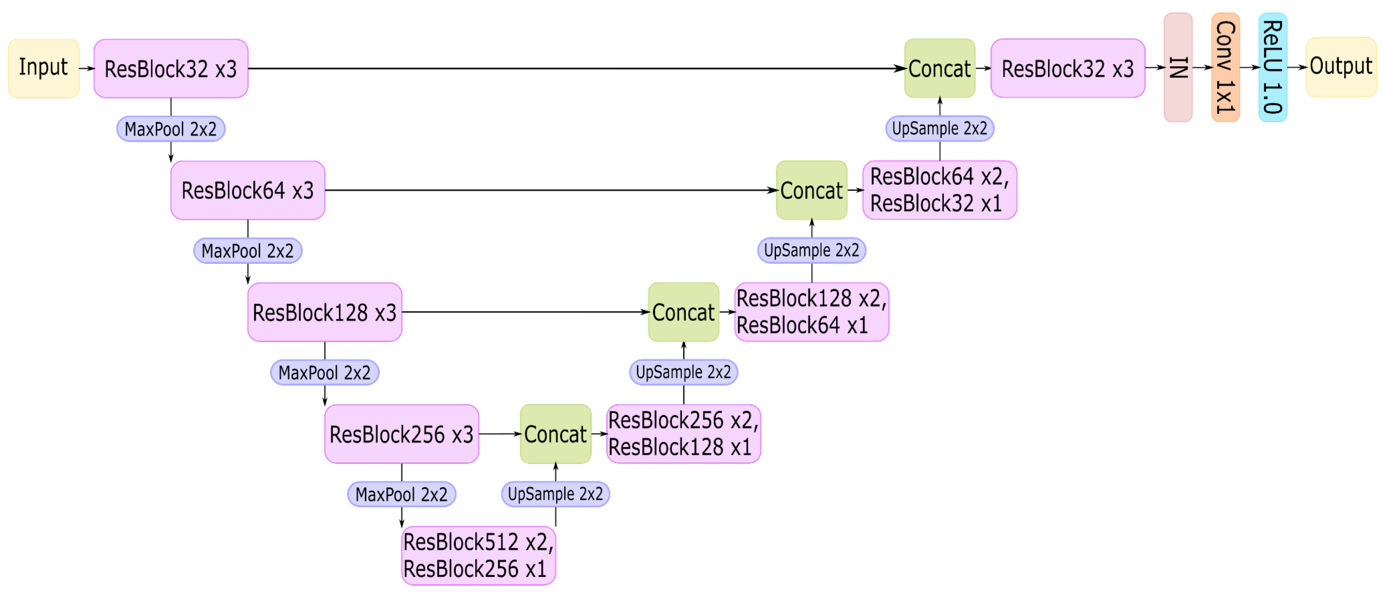
The overall architecture of our U-net model is shown in Figure 3. It consists of 5 levels; on each level, there are 3 residual blocks. On the downsampling path, each level’s output is saved and later concatenated to the input of its counterpart level on the upsampling path. The resolution of the feature tensor changes only when the level is changed. In order to perform the resolution change, max pooling and upsampling layers are used on downsampling and upsampling paths respectively. The final output of the network is activated by ReLU with a threshold of 1.
In order to find the optimal architecture of the neural network, we have tested different hyperparameters such as the number of residual blocks, the depth of the network and the number of feature channels after each block. Our goal was to maximize the quality of the resulting images using as few learnable parameters as possible. Our experiments have shown that decreasing the size of the network results in a significant drop in the quality of produced images and increasing the size of the network has a negative effect on the performance with marginal improvement in the quality.

2.3. Training Flow

The network is trained on multiple 256 × 256 patches taken from a single annual VIIRS NTL image. In order to get patches containing actual lights rather than a background, a quantile filter is used. This filter works as follows: it selects all pixels with intensity higher than a certain quantile of the radiance distribution within the VIIRS NTL image. Then patches containing only the selected pixels are produced. By having this filter, we can control the minimum radiance of the lights the network is trained on. For example, the quantile of 0.01 is used to select patches from low-radiance regions like the countryside, but when the quantile of 0.6 is used the patches will include major cities, gas flares, etc. So, we use the quantile filter to change the radiance of the data fed to the network on each epoch. This approach helps us to greatly reduce the oversaturation problem.
The training process consists of 20 epochs; training for more epochs increases test error. We gradually increase the quantile from 0.01 to 0.6 as an epoch number increases. Each epoch consists of 10 mini-epochs. On every mini-epoch, 1024 patches are generated by a quantile filter. Then data augmentation is performed to increase the number of patches in the training set. For augmentation we use rotations and flips.
We use Mean Absolute Error (MAE) as a loss function:
L M A E = 1 N 1 M n = 1 N   m = 1 M   | y n , m t r u e y n , m p r e d | ,
where y n , m t r u e is a “ground truth” value of the m-th pixel in the n-th image in the training batch (from the annual DMSP NTL data), y n , m p r e d is a value of the m-th pixel in the n-th image in the batch predicted by the network from VIIRS data, N is the total number of images in the batch, M is the total number of pixels in one image (patch).
We use Adam stochastic optimizer [18] with the default settings except for the learning rate. We use a cyclical exponential decay learning rate (2) with the initial learning rate = 0.001 and we configure it so that at the end of the epoch it will have a learning rate = 0.0002. At every epoch start, it is reset to the initial learning rate.
l r = l r i n i t   d ( s t e p / s t e p s t o t a l )   ,
where lr is a current learning rate, lrinit is an initial learning rate, d is a decay rate.
The whole training process takes about 10 h to complete on the NVIDIA Tesla V-100 graphics card. The training was conducted with Google Colab notebooks using virtual machine instances with GPU in Google cloud. Tensorflow machine learning platform was used to build and train the CNN.

2.4. Generation of Results

Since the whole composite of VIIRS data takes about 3 Gb, it is impossible to use the trained network directly on the data to produce DMSP-like imagery. Instead, we divide VIIRS data into overlapping patches of the size 256 × 256 with each pixel being covered by at least 4 patches and predict on these patches. It is necessary to use overlapping patches because of the visual errors, which may occur on the edges of non-overlapping patches. Then these overlapping patches are multiplied by a 256 × 256 filter with normally distributed coefficients and added together. The coefficients are added to the array of the same size as the full DMSP-like composite. Finally, the image obtained by adding overlapping patches is divided by the coefficients array to normalize the imagery to the original distribution of radiance values. This technique allows for the generation of DMSP-like imagery on a GPU with limited memory. It also tackles the problem of visual artefacts at the edges of the non-overlapping patches, yielding the result that has no visual artifacts presented by stitching.

3. Result

To test our model, we took certain points of interest, namely Las Vegas, Los Angeles, Moscow, and a gas flare in Venezuela (63.5635E, 9.6419N), which is the brightest point in the 2015 VIIRS data. This data was not seen by a network so it suits well for a testing purpose. For these spots, scatter plots were made. They can be seen in Figure 4. The plots on the Y-axis contain the pixel values for the original DMSP data, and on the X-axis the corresponding pixel values obtained using the neural network are shown. Linear regression and its 95% confidence interval have also been plotted to show the ongoing trends. Fraction shows the likelihood of the predicted pixel to have a certain value compared to the original DMSP value for that pixel.
To evaluate the quality of image translation more thoroughly, we have calculated the determination coefficient (R2) shown in Table 2. These coefficients are very close to 1 for all the spots, showing that the model predicts results that are close to the original DMSP data. Additionally, the same 2D histograms were plotted with a median, 2.5 percentile, and 97.5 percentile instead of linear regression slope and confidence intervals. They can be seen in Figure 5. We have made the same plots with linear regression and the median for the whole world. These can be accessed in Supplementary Materials. The overall R2 for the world DMSP-like and F15 radiances in 2015 is 0.94.
One of the most significant achievements of our model is that it yields images that visually appear very close to the DMSP data. This has never been achieved before in the previous papers on this topic. A comparison between the DMSP data and data that is generated by our model is presented in Figure 6. At first glance, it is almost impossible to distinguish between them and the difference lies in subtle things like a glow in the Los Angeles Bay area, which is slightly fainter in data generated by our model compared to the DMSP data. The model captured all main features of DMSP data like saturation in images and blur effect, generating these features from clear, high resolution, higher dynamic range images gathered from the VIIRS sensor.
To assess the quality of our model from one more perspective, we have plotted histograms for our test spots. In these histograms, we examine how values of original DMSP data and predicted from VIIRS data are distributed. Histograms are shown in Figure 7 and Figure 8. The difference between these figures is that in Figure 8 data is plotted for mid-high range pixel values. One can see that distribution of values is quite close between original and predicted data but there are some differences. In Figure 7 the most obvious difference occurs near values close to 0. Neural Network predicts values 1–2 when the background removed annual DMSP images do not have these values. It happens because when DMSP data is processed the low-light values 1–2 are set to background 0 and the NN did not catch this peculiarity.

4. Discussion

The main strengths of our approach are visual results that have never been achieved before and the good metrics performance of the model. The quality of produced images is sufficient for them to be visually indistinguishable from the real DMSP data. The determination coefficient of the model is very close to 1 in all the test spots; distribution of the generated data in the midrange pixel values is similar to the original DMSP. However, the questions may arise regarding our strategy to downgrade high quality data from the modern satellites instead of upgrading the old one and to use the local context around the predicted pixel with a non-linear NN-based image filter instead of the much simpler pixel-to-pixel regression.

4.1. Why Are We Converting VIIRS to DMSP Radiances and Not Vice Versa?

We are converting VIIRS radiances to DMSP DNs for two reasons: (1) the saturation limit of the VIIRS sensor is higher than that of the and (2) spatial resolution of the VIIRS sensor is five times better than that of the DMSP. For those brightness values that exceed the saturation threshold DMSP, there is nowhere to take values. It is possible to filter out (smooth) high spatial frequencies from the VIIRS image, but there is no deterministic way to add detail to the DMSP one. This can be shown by the comparison with the results presented in [10]. In this work, an extended time series (2000–2018) of nighttime data similar to NPP-VIIRS was constructed using cross-sensor calibration using annual DMSP-OLS data for 2000–2012. and monthly SNPP-VIIRS data for 2013–2018. A key feature of this approach was the improvement of the image by using the vegetation index and an artificial neural network with an autoencoder model. The result of this work is a set of annual NTL files in open access.
We have compared the results of Chen et al. [10] for 2015 with the annual VNL v2.0 data for 2015 published by EOG [2]. We also have made a similar comparison for the result of our 2015 cross-satellite calibration, comparing it with the annual DMSP data for 2015.
Figure 9 shows the percentage histograms of the pixel brightness in Sicily. We chose Sicily for cross-comparison, since in this region the brightness of the night lights changes little throughout the year [19]. The percentile histogram does not show the absolute number of values that fall into the bin but the percentage of their total number. We switched to percentiles because the data [2,10] at 15 arcsec. Latitude–longitude grid are in slightly different projections: 0.0045 deg. step vs. 0.0042 deg. We see (right histogram) that the higher the brightness, the greater the discrepancy in the number of pixels between the Chen’s data [10] and the VIIRS NTL. At the same time (left histogram), no such deviation is observed for the DMSP radiances predicted with NN from VIIRS NTL.
When analyzing temporal dynamics of city lights, errors in the highest brightness values can lead to significant inaccuracies. We performed the following analysis: (1) randomly selected 13 large cities with bright lighting (Paris, Madrid, Lisbon, Prague, Minsk, Moscow, Shanghai, Tokyo, Las Vegas, Mexico City, Rome, New Delhi, Wuhan); (2) took squares of size 0.2 × 0.2 degrees in the city downtown; (3) for each of the four datasets, the values of the brightness of the pixels were averaged in the selected squares; (4) calculated the ratio of the brightness of the predicted data to the original; (5) made the scatterplots of the predicted vs. observed ratios (Figure 10). The scatterplots show that the average brightness for city centers according to [10] can be two times lower compared to the VIIRS NTL v2.0. At the same time, the ratio of the NN predicted DMSP brightness to the observed DMSP NTL for city centers is close to 1.
We have also noticed that the background (no lights) in [10] is filtered with a higher threshold compared to VIIRS NTL v2.0. For example, in Sicily (Figure 11) the NTL map built from [10] has a significantly larger area of the background (highlighted in green) compared to VIIRS NTL. Contrary to that, the background area for the NN prediction of DMSP-like radiances is 4% smaller than the background of the annual DMSP NTL in 2015.

4.2. Can We Use Pixel-to-Pixel Regression for Converting VIIRS Radiance to DMSP?

We have compared our result with the results obtained in [11]. As part of this work, the authors intercalibrated the DMSP data between years (for the years when the DMSP observations were made) and simulated the annual DMSP-like radiances from VIIRS (for those years in which there were no DMSP observations) with sigmoid regression. The result of this work is also a set of annual NTL files in open access. We took the simulation result for 2015 from [11] and compared it with the annual DMSP F15 NTL map for 2015 (link to open annual DMSP data for 2015 or the form where this data can be ordered). For comparison, we plotted histogram of pixel brightness in Sicily resulting from both cross-calibration methods in Figure 12. It shows that the consistency of histograms is higher for our approach.
For the NN predictions, we have plotted sums of lights and pixel brightness histograms in Sicily (Figure 13 and Figure 14) for the years from 2013 to 2019 where the observed SNPP-VIIRS and DMSP F15 datasets overlap. Both the sum of lights in Figure 13 and their statistical distributions in Figure 14 match well for all the years. The difference in sum of lights for 2013–2019 does not exceed 15%, with the biggest difference happening in 2013.

5. Conclusions

This work provides a method based on Convolutional Neural Networks to generate analogs of DMSP data from VIIRS data. Our solution proves to work in various geographical areas. Usage of CNN for this purpose provides great accuracy (0.96 < R2 < 0.99) and produces images that are visually indistinguishable from original DMSP images. Our method preserves the distribution of midrange values and proves to work well in real-world scenarios. All this makes it possible to complete long-term NTL series and to utilize both DMSP and VIIRS data in potential studies. In order to make usage of the CNN as easy as possible, in the Supplementary Materials to this paper we will publish the weights of the trained neural network and the source code to generate DMSP-like NTL maps from VIIRS with this network. Observed DMSP and VIIRS nighttime lights for 2012–2019 as well as the NN predicted DMSP-like data are in open access from the EOG web site at Colorado School of Mines.

Supplementary Materials

All the plots and histograms alongside the weights for neural network and source code are available at https://github.com/megavaz/CNN-DMSP-generation (accessed on 8 December 8 2021).

Author Contributions

Conceptualization, M.Z.; methodology, software and validation, D.N. and A.P.; data curation, C.E., T.G. and F.-C.H.; writing—original draft preparation, D.N., A.P., M.Z.; writing—review and editing, T.G. and M.Z. All authors have read and agreed to the published version of the manuscript.

Funding

This research was funded by AGENCE FRANCAISE DE DEVELOPPEMENT (AFD), a public body whose registered office is at 5 Rue Roland Barthes, 75012 Paris, France registered on the Paris Trade and Companies Register under number B 775 665 599. Siret Number: 77566559900129; Chorus Number: PAR-IRS-003; Purchase order number: 21004880.

Institutional Review Board Statement

Not applicable.

Informed Consent Statement

Not applicable.

Data Availability Statement

Publicly available datasets were analyzed in this study. All the NTL data used for training and validation of the neural network are available at https://eogdata.mines.edu/products/vnl/ (accessed on 8 December 8 2021) and https://eogdata.mines.edu/products/dmsp/ (accessed on 8 December 2021).

Conflicts of Interest

The authors declare no conflict of interest.

References

  1. Elvidge, C.D.; Baugh, K.E.; Kihn, E.A.; Kroehl, H.W.; Davis, E.R. Mapping city lights with nighttime data from the DMSP Operational Linescan System. Photogramm. Eng. Remote Sens. 1997, 63, 727–734. [Google Scholar]
  2. Elvidge, C.D.; Zhizhin, M.; Ghosh, T.; Hsu, F.-C.; Taneja, J. Annual Time Series of Global VIIRS Nighttime Lights Derived from Monthly Averages: 2012 to 2019. Remote Sens. 2021, 13, 922. [Google Scholar] [CrossRef]
  3. Levin, N.; Kyba, C.; Zhang, Q.; Sanchez de Miguel, A.; Roman, M.; Li, X.; Portnov, B.; Molthan, A.; Jechow, A.; Miller, S.; et al. Remote sensing of night lights: A review and an outlook for the future. Remote Sens. Environ. 2020, 237, 111443. [Google Scholar] [CrossRef]
  4. Elvidge, C.; Baugh, K.; Zhizhin, M.; Hsu, F. Why VIIRS data are superior to DMSP for mapping nighttime lights. Proc. Asia-Pac. Adv. Netw. 2013, 35, 62–69. [Google Scholar] [CrossRef] [Green Version]
  5. Mills, S.; Miller, S. VIIRS Day/Night Band—Correcting Striping and Nonuniformity over a Very Large Dynamic Range. J. Imaging 2016, 2, 9. [Google Scholar] [CrossRef] [Green Version]
  6. Pandey, B.; Zhang, Q.; Seto, K. Comparative evaluation of relative calibration methods for DMSP/OLS nighttime lights. Remote Sens. Environ. 2017, 195, 67–78. [Google Scholar] [CrossRef]
  7. Li, X.; Chen, X.; Zhao, Y.; Xu, J.; Chen, F.; Li, H. Automatic intercalibration of night-time light imagery using robust regression. Remote Sens. Letters. 2013, 4, 45–54. [Google Scholar] [CrossRef]
  8. Zheng, Q.; Wang, K. Developing a new cross-sensor calibration model for DMSP-OLS and SuomiNPP VIIRS night-light imageries. ISPRS J. Photogramm. Remote Sens. 2019, 153, 36–47. [Google Scholar] [CrossRef]
  9. Tu, Y.; Zhou, H.; Lang, W.; Chen, T.; Li, X.; Xu, B. A novel cross-sensor calibration method to generate a consistent night-time lights time series dataset. Int. J. Remote Sens. 2020, 41, 5482–5502. [Google Scholar] [CrossRef]
  10. Chen, Z.; Yu, B.; Yang, C.; Zhou, Y.; Yao, S.; Qian, X.; Wang, C.; Wu, B.; Wu, J. An extended time-series (2000–2018) of global NPP-VIIRS-like nighttime light data. Earth Syst. Sci. Data 2020, 13, 889–906. [Google Scholar] [CrossRef]
  11. Li, X.; Zhou, Y.; Zhao, M.; Zhao, X. A harmonized global nighttime light dataset 1992–2018. Sci. Data 2020, 7, 168. [Google Scholar] [CrossRef] [PubMed]
  12. Ronneberger, O.; Fischer, P.; Brox, T. U-Net: Convolutional Networks for Biomedical Image Segmentation. LNCS 2015, 9351, 234–241. [Google Scholar] [CrossRef] [Green Version]
  13. He, K.; Zhang, X.; Ren, S.; Sun, J. Deep Residual Learning for Image Recognition. In Proceedings of the 2016 IEEE Conference on Computer Vision and Pattern Recognition (CVPR), Las Vegas, NV, USA, 27–30 June 2016; pp. 770–778. [Google Scholar] [CrossRef] [Green Version]
  14. Annual VIIRS Nighttime Light Composites. Available online: https://eogdata.mines.edu/products/vnl/ (accessed on 16 March 2021).
  15. Baugh, K.; Elvidge, C.; Tilottama, G.; Ziskin, D. Development of a 2009 stable lights product using DMSP-OLS data. Proc. Asia-Pac. Adv. Netw. 2010, 30, 114–130. [Google Scholar] [CrossRef]
  16. Elvidge, C.; Baugh, K.; Zhizhin, M.; Hsu, F.; Tilottama, G. VIIRS night-time lights. Int. J. Remote Sens. 2017, 38, 1–20. [Google Scholar] [CrossRef]
  17. Ulyanov, D.; Vedaldi, A.; Lempitsky, V. Instance Normalization: The Missing Ingredient for Fast Stylization. arXiv 2016, arXiv:1701.02096. [Google Scholar]
  18. Kingma, D.; Ba, J. Adam: A Method for Stochastic Optimization. arXiv 2014, arXiv:1412.6980v9. [Google Scholar]
  19. Hsu, F.-C.; Baugh, K.E.; Ghosh, T.; Zhizhin, M.; Elvidge, C.D. DMSP-OLS Radiance Calibrated Nighttime Lights Time Series with Intercalibration. Remote Sens. 2015, 7, 1855–1876. [Google Scholar] [CrossRef] [Green Version]
Figure 1. DMSP and JPSS satellites equatorial crossing times for ascending and descending orbits with nighttime data.
Remotesensing 13 05026 g001
Figure 2. The architecture of a residual block. IN is Instance Normalization, ReLU is Rectified Linear Unit, Conv is convolution layer, Add is the addition of two tensors, Dropout has a rate of 0.2.
Remotesensing 13 05026 g002
Figure 3. U-net architecture is used to perform cross-calibration from VIIRS data to the analog of DMSP data. ResBlockN xM is M residual blocks stacked one after another, every convolutional layer in these blocks produces N feature channels; MaxPool is a max pooling layer that is used to reduce the resolution of features; UpSample is an upsampling layer, it is used to increase the resolution of features; Concat is a concatenation operation, it is performed on channels axis; the last 3 layers prior to output are instance normalization, 1 × 1 convolution and ReLU activation with a threshold 1.
Remotesensing 13 05026 g003
Figure 4. Scatter plots for various spots: (a) Las Vegas; (b) Los Angeles; (c) Moscow; (d) Brightest gas flare in Venezuela. Linear Regression (LR in legend) with coefficient a and 95% confidence intervals for it are plotted. Fraction shows the likelihood of predicted pixels to have a certain value compared to the original DMSP values.
Remotesensing 13 05026 g004aRemotesensing 13 05026 g004b
Figure 5. Scatter plots for various spots: (a) Las Vegas; (b) Los Angeles; (c) Moscow; (d) Brightest gas flare in Venezuela. Median, 2.5 percentile and 97.5 percentile are plotted. Fraction shows the likelihood of predicted pixels to have a certain value compared to the original DMSP values.
Remotesensing 13 05026 g005
Figure 6. Visual comparison between certain spots: (a) Las Vegas; (b) Los Angeles; (c) Brightest gas flare in Venezuela. On the left original VIIRS images, in the center images generated by the CNN, on the right original DMSP images.
Remotesensing 13 05026 g006aRemotesensing 13 05026 g006b
Figure 7. Histograms for pixel values for various spots: (a) Las Vegas; (b) Los Angeles; (c) Moscow; (d) Brightest gas flare. Original DMSP data is plotted in blue, data that was predicted by our model is plotted in orange. Probability shows the number of pixels with that value divided by the number of all the pixels. Pixels with value 0 are truncated.
Remotesensing 13 05026 g007
Figure 8. Histograms for midrange pixel values for various spots: (a) Las Vegas; (b) Los Angeles; (c) Moscow; (d) Brightest gas flare. Original DMSP data is plotted in blue, data that was predicted by our model is plotted in orange. Probability shows the number of pixels with that value divided by the number of all the pixels.
Remotesensing 13 05026 g008
Figure 9. Percentile histograms of brightness distribution for Sicily in 2015: according to the NN-predicted and observed DMSP data (left), according to the model by Chen et al. [10] and SNPP-VIIRS NTL v2.0 [2] (right).
Remotesensing 13 05026 g009
Figure 10. Ratio of city-center brightness between predicted and observed data: for Chen et al. VIIRS from DMSP [10] (top), for our calibration method (bottom).
Remotesensing 13 05026 g010
Figure 11. Annual NTL maps in Sicily for 2015 based on SNPP-VIIRS NTL v2.0 [2] (upper left), the model by Chen et al. [10] (lower left), on DMSP F15 (upper right) and NN-predicted from VIIRS NTL (lower right). Background areas with zero radiance values are shown in green.
Remotesensing 13 05026 g011
Figure 12. Histograms of NTL brightness for Sicily in 2015: according to the NN-predicted (left), to the cross-calibration by Li et al. [11] and SNPP-VIIRS NTL v2.0 [2] (right) and the observed DMSP radiances.
Remotesensing 13 05026 g012
Figure 13. Sum of nighttime lights for Sicily by year for the observed DMSP F15 data for 2013–2019 and for the NN predicted brightness from the corresponding annual VIIRS NTL v2.0.
Remotesensing 13 05026 g013
Figure 14. Histograms of the annual NTL brightness in Sicily from 2012 to 2019, made for the observed DMSP F15 data for 2013–2019 (blue bars) and for the NN predicted brightness from the corresponding annual VIIRS NTL v2.0 (orange bars).
Remotesensing 13 05026 g014
Table 1. Difference between DMSP-OLS and SNPP-VIIRS sensors.
VariableDMSP-OLSSNPP-VIIRS
Builder/OperatorUS Air ForceNASA–NOAA Joint Polar Satellite System (JPSS)
OrbitPolar solar-synchronous–850 km altitude, 98.8 degree inclination, 102 minPolar solar-synchronous–827 km altitude, 98.7 degree inclination, 102 min
Swath3000 km3000 km
Nighttime overpass (local time)~19:30 until 2013, ~4:30 after 2012~01:30 local time
Low light imaging band passPanchromatic 0.5 to 0.7 umPanchromatic 0.5 to 0.9 um
Ground footprint5 km × 5 km at nadir742 m × 742 m
Quantization (dynamic range)6 bit14 bit
SaturationCommon in urban coresNo saturation
Low light imaging detection limit~ 5 × 10⁻¹⁰ W/cm2/sr~ 2 × 10⁻¹¹ W/cm2/sr
CalibrationNone for low light imagingSolar diffuser
Future continuityProgram decommissionedJPSS has launched the second satellite NOAA-20. The third satellite is scheduled to be launched in 2022
Table 2. Correlation between original and predicted images.
SpotR2 (Determination Coefficient)
Las Vegas0.99
Los Angeles0.99
Moscow0.97
Brightest flare0.96
Global image0.94
Publisher’s Note: MDPI stays neutral with regard to jurisdictional claims in published maps and institutional affiliations.

