Article

An Effectively Dynamic Path Optimization Approach for the Tree Skeleton Extraction from Portable Laser Scanning Point Clouds

1
College of Information Science and Technology, Nanjing Forestry University, Nanjing 210037, China
2
College of Landscape Architecture, Nanjing Forestry University, Nanjing 210037, China
*
Author to whom correspondence should be addressed.
Remote Sens. 2022, 14(1), 94; https://doi.org/10.3390/rs14010094
Submission received: 23 November 2021 / Revised: 12 December 2021 / Accepted: 22 December 2021 / Published: 25 December 2021
(This article belongs to the Section Forest Remote Sensing)

Abstract

:
One key step to the tree structure study is skeleton processing. Although there are lots of extraction approaches, the existing methods have paid less attention to extraction effectiveness, which highly use redundant points to formulate the skeleton and bring difficulties to the subsequent 3D modeling. This work proposes a four-step framework for the purpose of skeleton extraction. Firstly, candidate skeleton points are filtered from input data based on the spatial slice projection and grouped using the Euclidean distance analysis. Secondly, a key dynamic path optimization step is used to formulate a tree skeleton using the candidate point information. Thirdly, the optimized path is filled by interpolating points to achieve complete skeletons. Finally, short skeletons are removed based on the distance between branching points and ending points, and then, the extraction skeletons are smoothed for improving the visual quality. Our main contribution lies in that we find the global minimization cost path from every point to the root using a novel energy function. The formulated objective function contains a data term to constrain the distance between points and paths, and a smoothness term to constrain the direction continuities. Experimental scenes include three different types of trees, and input point clouds are collected by a portable laser scanning system. Skeleton extraction results demonstrate that we achieved completeness and correctness of 81.10% and 99.21%. respectively. Besides, our effectiveness is up to 79.26%, which uses only 5.82% of the input tree points in the skeleton representation, showing a promising effective solution for the tree skeleton and structure study.

1. Introduction

Nowadays, the Light Detection and Ranging (LiDAR) technique has played a significant role in mapping 3D space information of vegetation, such as crown delineation [1,2], wood–leaf separation [3], and tree segmentation [4]. In the field of vegetation modeling and analysis, one fundamental step is tree skeleton extraction, which vitally does the benefits tree branch structure study.
Different from building footprint detection [5], the tree skeleton belongs to those which are non-rigid and is present in various geometric shapes occluded by foliage. Recently, portable laser scanning systems (PLS) have become increasingly more mature, which provide data in dense point-cloud sets and are flexible to capture the region of interest of street tree information. Moreover, portable laser scanning systems do not expect users with professional surveying experience, which brings PLS more chances in 3D structure research.
Currently, most of the existing skeleton extraction methods have been proposed for terrestrial laser scanning (TLS) and vehicle laser scanning point clouds, which requires researchers to develop new skeleton extraction approaches for PLS point clouds. This work aims to address the potential issues that lie in the existing approaches, that is, low effectiveness, completeness, and correctness, in PLS point cloud processing. Contributions are outlined as follows: (1) we propose an effective skeleton extraction framework for the PLS point clouds, and (2) we develop a new dynamic path approach for the skeleton optimization. The skeleton extraction plays an important role in 3D tree modeling and the branch trend change study, which provides paths for branch tracking and benefits to researchers related to structural and growth trend analysis.

2. Related Works

Recently, many approaches have appeared for tree skeleton extraction from point clouds. A straightforward idea is to extract the skeleton based on the geometrical and topological feature information from stem points.
In the method of the Ref. [6], they intended to obtain skeleton information from tree stems, which were modeled by fitting a series of cylinders based on the random sample consensus approach. The Ref. Zhang et al. [7] proposed a segment-based method for efficient stem detection at the plot level, which is based on the curvature feature of the points. The Ref. Xu et al. [8] detected stems by combining geometrical and topological features of points, and then used feature selection methods to input optimal features for the later Support Vector Machine (SVM) classification [9,10] to classify stem points. Those stem-based methods are efficient in obtaining trees’ nonphotosynthetic components, but fail to achieve fine skeletons for modeling.
In the method of the Ref. [11], they first generated candidate skeletons by thinning voxels. Then, skeletons were transformed into a mathematical tree and pruned by using their biologically inspired features. Although their method achieves fine skeletons, it requires a learning process to capture linearity information from points, which is also a challenge in 3D point cloud processing. The Ref. Zhang et al. [12] introduced a method for extracting topological and structural information of tree branches. First, point clouds are clustered, and the neighborhood relationship between each cluster is used to determine the connectivity attributes. Then, they approximate each group as a cylinder with a different radius, length, and direction for reconstruction. This method has achieved a detailed skeleton from apple trees, but the results highly rely on the setting of the five input parameters.
In order to address potential issues caused by local minimization, such as how extraction results are sensitive to parameter-setting and easily fall into local optimum, researchers have tried to search for global optimization. In the work of the Ref. [13], the authors formulated a graph by connecting neighboring points, and then they extracted a skeleton based on Dijkstra’s shortest path algorithm. Although this method extracts various skeletons from graphs, cycle paths appear in the complex branch structures. The Ref. Bucksch and Lindenbergh [14] represented skeletons as a graph, and organized the input points as octree-graphs to eliminate cycles in the graph. This method removes cycle paths in the skeleton but fails to remove those incorrectly initialized false paths. The Ref. Livny et al. [15] reconstructed skeletal structures of trees based on a series of global optimizations. They first represented each reconstructed tree by using a spatially embedded and connected directed acyclic graph. Then, they calculated the importance weights of vertices based on the sizes of their subtrees. Their results correctly achieve skeletal structures from noisy point data, but the accuracy is highly subjected to their criteria. In order to obtain complete skeletons, the Ref. Wang et al. [16] first obtained the approximate tree skeleton from a distance minimum spanning tree and then defined the stretching directions of the branches. Although they succeeded in recovering the missing data by adding paths along with the detected stretching directions, one potential issue lies in the dominant direction calculation, where it is easy to miss small skeletons in the merging step. The Ref. Du et al. [17] extracted an initial tree skeleton by establishing a minimum spanning tree first. Then, they pruned the initial tree skeleton by iteratively removing redundant components. This method succeeds in proving high-quality skeletons in various tree points but generates several false skeletons in crowns caused by their Delaunay triangulation in graph initialization.
Although the above-mentioned approaches have provided good skeleton extraction results, there is still one key issue that needs to be solved, that is, how to use as few points as possible to formulate the skeleton. As shown in the Refs. [13,14], they constructed graphs based on neighboring points, which use as much information as possible for subsequent branch detection, easily resulting in redundant paths. If one uses fewer neighbor points, branches tend to be formulated directly from neighbors to their closest points, causing false paths, as shown in the Ref. Du et al. [17]. This will be addressed by formulating a novel energy function for searching the optimal path rather than considering the Euclidean distance only.

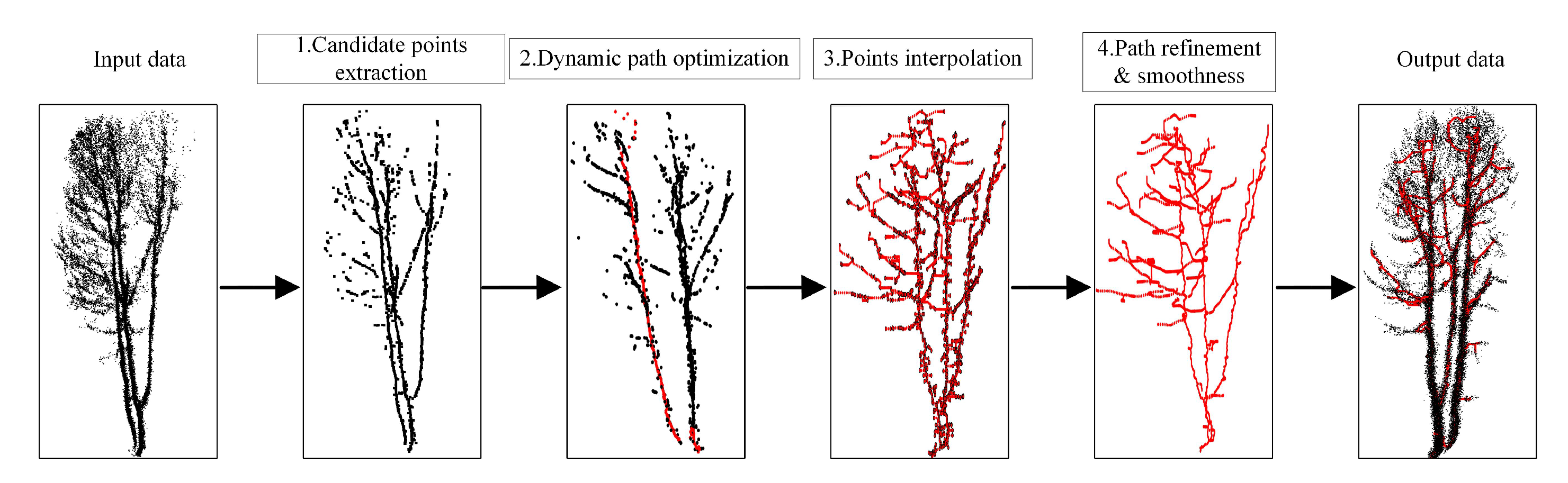
3. Tree Skeleton Extraction

As shown in Figure 1, there are four main steps in the proposed tree skeleton extraction framework. Input tree point clouds are shown in the left of Figure 1. The first step is to extract candidate points as stem centers from input data. Because the color information of point clouds needs a registration step and the intensity information needs a calibration step, we only use the coordinate x , y , z information in the extraction. The second step is the key process to dynamically find the optimal path for the later skeleton based on the formulated energy function. The third step is to complete skeletons by interpolating points along the optimal path. The last step is to refine the path by removing error branches and smoothing correct skeletons. The overlap between skeleton and input data is visualized in the right of Figure 1. The following section shows details of each step.

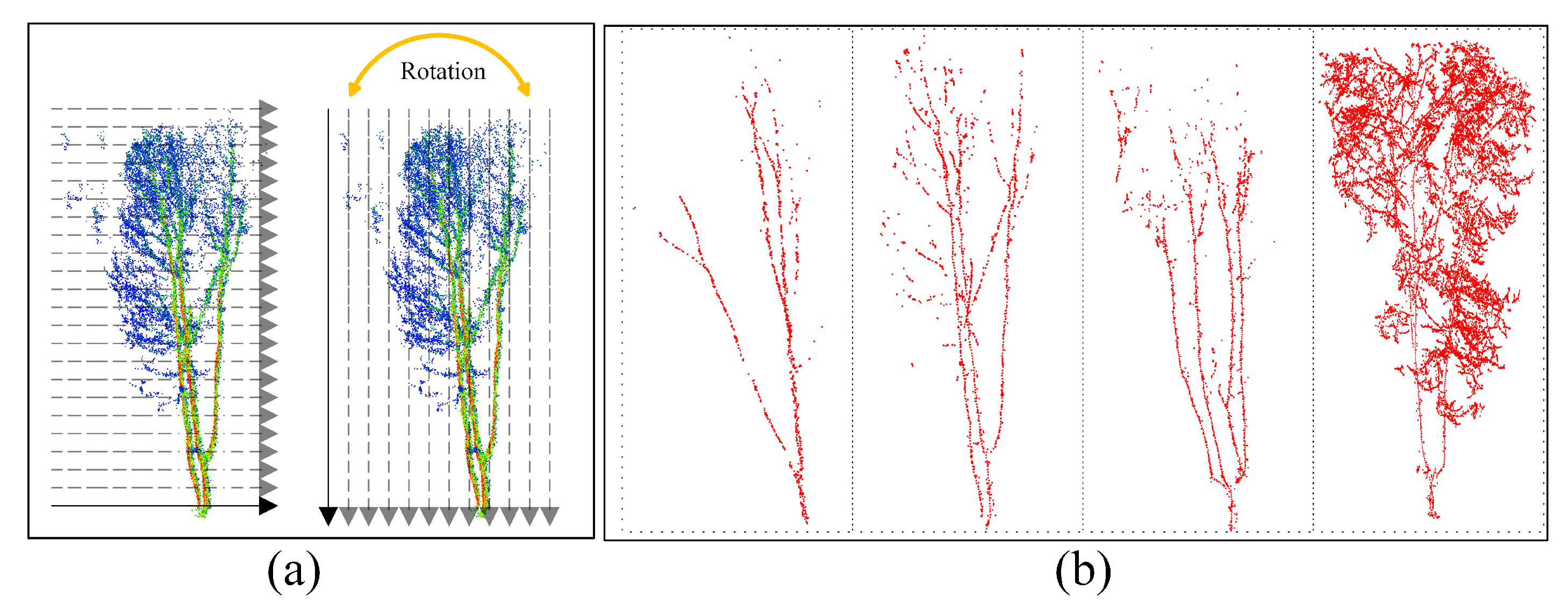
3.1. Candidate Point Extraction

Point clouds are unorganized and massive; therefore, we first try to find candidate points as input for the later process, which significantly reduces the point cloud computation.
Our candidate points are achieved based on the slice processing and clustering step. As shown in Figure 2a, we slice input data vertically to find candidate points in the Z-axis direction. In order to obtain candidate points in the X-axis and Y-axis horizontally, rather than calculating projection planes, we rotate input data based on the transformation matrix, as shown in Equation (1). After that, we use the Euclidean distance information to group points into regions in the clustering process and regard centers as the output of candidate point extraction. As shown in the first three columns of Figure 2b, we obtain different center points from the slice projection. More projection planes will bring more candidate points. In order to obtain tree points from different directions, we rotate input points based on our transformation matrix. ϕ is set by users based on the number of divisions. In our work, the number of the slice division is 2 Π 6 . At the end of this step, we merge all candidate points into the output of this step, as shown in the fourth column of Figure 2b.
R = cos ϕ sin ϕ 0 sin ϕ cos ϕ 0 0 0 1

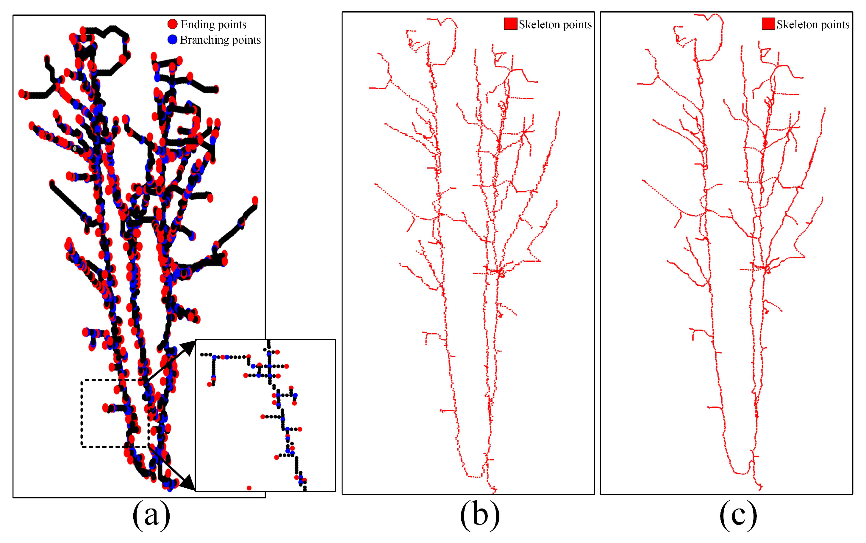
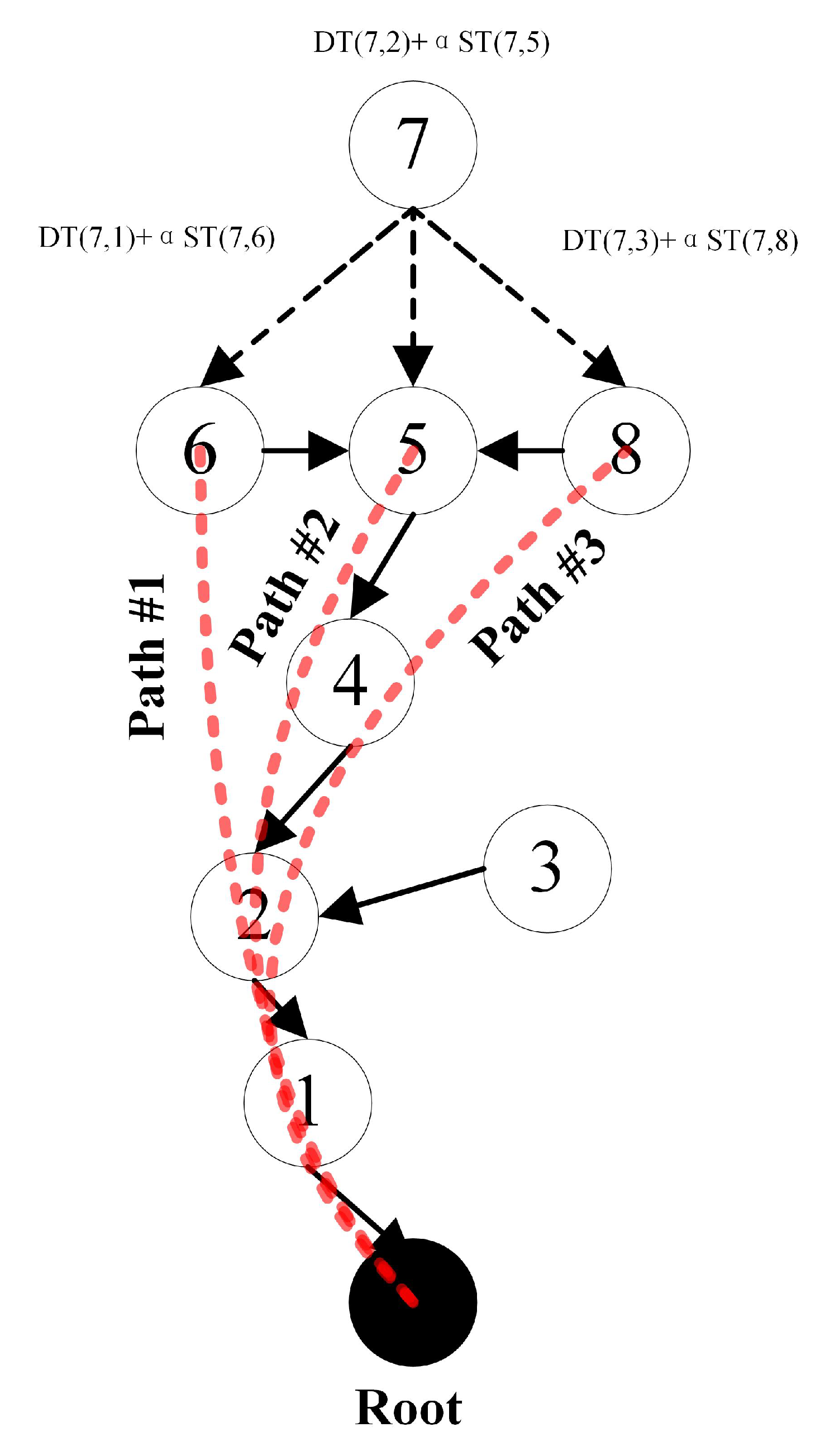
3.2. Dynamic Path Optimization

Now, the key issue lies in how to find the optimal path from current points to the root. Our idea is to evaluate the cost of each path from the current point to the root based on a novel energy function. The path with the minimum cost corresponds to the optimal branch for the current point. The challenge is that there are numerous paths from the current node to the root, therefore, it is difficult to calculate the cost for each path. The following proposes a dynamic path optimization method to solve this issue in polynomial time.
After we obtain candidate points, the key step is to connect those points as skeletons. Therefore, we define energy function, including a data term and a smoothness term, to evaluate the path in the candidate point connection. The data term is to measure how well a point p i fits into the current path l based on the Euclidean distance, and the smoothness term is to measure the direction continuous of the path, as shown in Equation (2).
E = M i n i = 1 m D T p i , l + { p i , p j } N , p j l α · S T p i , p j ,
where
D T ( p i , l ) = min d i s p i , l , c , S T ( p i , p j ) = sin V i , V j
In Equation (3), c is a constant in our work, that is, 0.2, and V i is the dominate direction vector of the current point p i . α is a coefficient to the balance data term and smoothness term, that is, 1. The estimation of the direction vector is based on the neighbor points of p i . Similarly, V j is the direction vector of the point p j . p j and p i are points from the neighboring set N (the spatial closest 30 points) on the path l.
Figure 3 demonstrates the search of the optimal path for the current node #7. To search the path for this node, we are required to calculate the energy cost of adding node #7 to different paths. The path optimization is based on the dynamic programming strategy, which is shown in Algorithm 1.
In Algorithm 1 step 3, M A X _ V a l u e is an appropriately large value, that is, FFFF for 2 bytes. In Algorithm 1 step 4, an optimal point means the point that we have already found an optimal path from this node to the chosen root. j * is a new point, which indicates we have found the minimum cost path from j * to the optimal path. In the algorithm, we enlarge the optimal point set fd in the loop operation. i * shows the neighbor point of j * in the optimal path, which is used for the backtracking process to achieve the whole optimal path. It is worth noting that our goal is to update fb and tb . We move elements from tb to fb . Therefore, tb will be an empty set and all points will be added in fb . For each point from tb , before the moving, its previous node should be from fb .
Algorithm 1 Dynamic Path Optimization.
  • Input: The matrix D to measure the distance between every two points, which is calculated by the sum of the data term and smoothness term in Equation (3);
  • Output: The Vector Path to be dynamically optimized;
1:
Initialize the cost of an optimal path from root for each point p i as d i = 0 ;
2:
repeat
3:
    Set the minimum cost of the current path as M I N M A X _ V a l u e ;
4:
    Formulate all optimal points into the set fb ;
5:
    Formulate all non-optimal points into the set tb ;
6:
    for Each i fb  do
7:
        Formulate neighbors of i into the set N ;
8:
        for Each j tb  do
9:
           if  j N then return D i s D { i , j , l }
10:
           end if
11:
            D i s _ f u l l D i s + d i
12:
           if  D i s _ f u l l < M I N  then return  M I N D i s _ f u l l , i * i , j * j
13:
           end if
14:
        end for
15:
    end for
16:
     d j * M I N
17:
    Add j * into the set fb ;
18:
     Path j * i *
19:
until tb is empty

3.3. Points Interpolation

As we know, skeleton points can be missing due to occlusion or incomplete data. Therefore, we reorganize the above obtained path points to complete skeletons. As shown in the middle of Figure 4, spatially close points in region A (a sphere with a radius of 0.05 m) will be regarded as duplicate points and removed in this step. Then, we interpolate points between those candidate points with a large Euclidean distance directly. We arrange the distance between each two skeleton points with the same value, as shown in the right of Figure 4. Since the distance between each of the two points is the same, the following path refinement becomes easy to conduct.

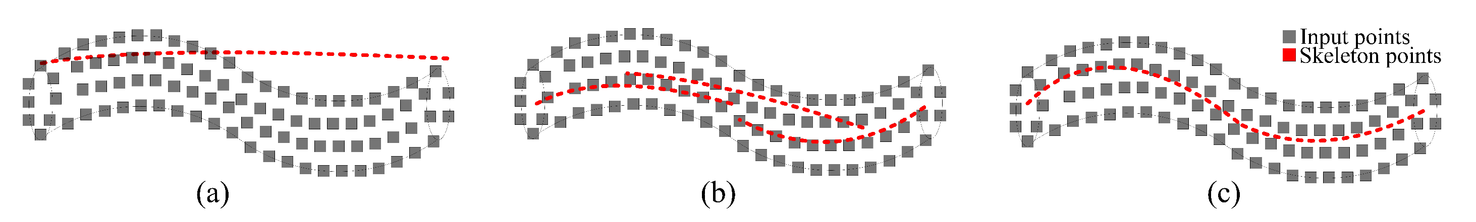
3.4. Path Refinement and Smoothness

In order to conduct the skeleton refinement, we classify input points as ending points and branching points. Ending points mean that there is no path out from this node, and branching points mean that there are more than one path out from this node. As shown in Figure 5a, we detect all branching points and ending points by examining the output of each node. For each path segment, that is, from the ending point to a branching point, if the length of a path is small, this path will be removed. We set the least path length as no less than five points empirically. Path refinement results are shown in Figure 5b. In order to improve the visual quality of skeleton, we smooth the achieved path based on the following Equations (4) and (5).
L = p i + 1 ( x , y , z ) p i ( x , y , z ) 2 + p i 1 ( x , y , z ) p i ( x , y , z ) 2
p i = p i + λ · L
The difference between two neighboring points p i + 1 and p i in Equation (4) is the 3D coordinate difference. In Equation (5), λ is a coefficient to balance the smoothness result, which is fixed as 0.1 in our work. In the implementation, we smooth all points one by one in each iteration. Usually, after 5–6 times of the smoothness process, we can get results, as shown in Figure 5c.

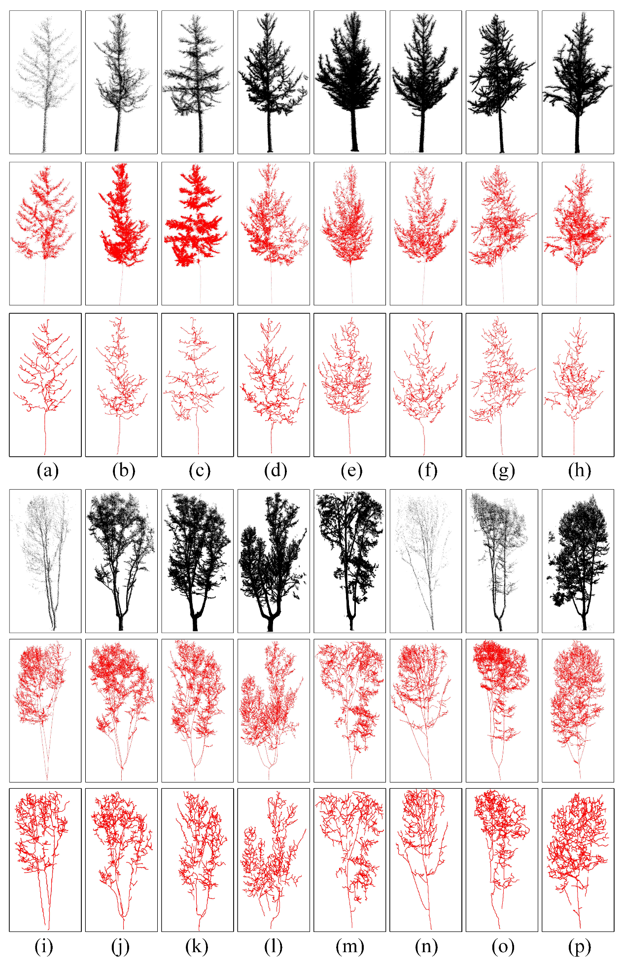
4. Experiments and Results

This section tests the proposed framework on portable laser scanning data. Data are collected by GeoSLAM ZEB-HORIZON as shown in Figure 6, which scans points at 300,000 points per second at the field of view 360 × 270 . This scanner is quite easy to use and suitable for the point collection of street trees. The input scene is located at Nanjing Forestry University, and Linggu Temple, Nanjing, China. Roads are covered by deciduous street trees, including Prunus serrulata, as shown in Figure 6a–c, Ginkgo biloba L., as shown in Figure 6d–h and Platanus acerifolia, as shown in Figure 6i–p. The following section includes both the visual evaluation to qualitatively demonstrate our tree skeleton extraction and the accuracy evaluation to quantitatively show the superiority in terms of the completeness, correctness, and effectiveness.

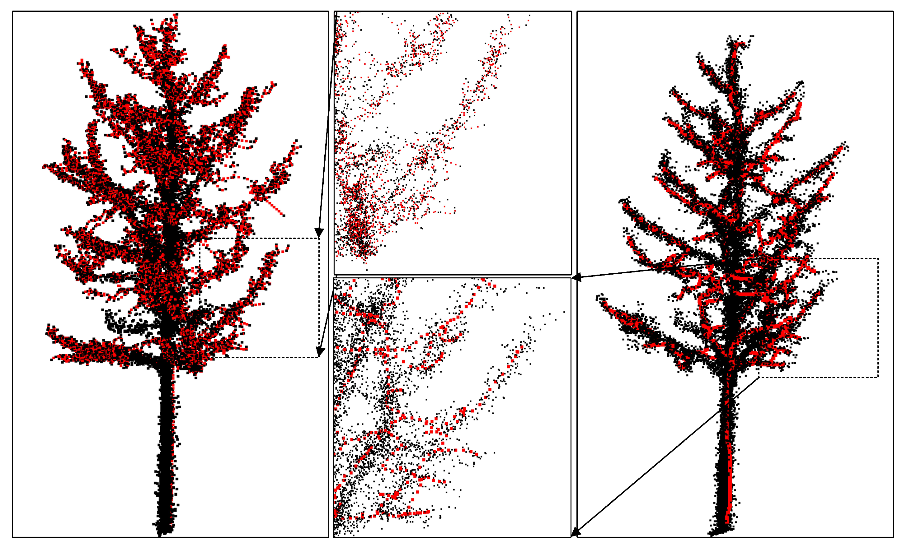
4.1. Visual Evaluation

Our extraction results are shown in Figure 6. We have succeeded in obtaining points from the first branching order and most points from the second branching order. Branch structures are demonstrated clearly in the extraction, including the basic topological and geometrical information. The first row of Figure 6a–h shows the input data. The second row of Figure 6a–h shows results from AD (accurate and detailed) [17], and the third row of Figure 6a–h shows our results.
The comparison of our approach and AD shows that we have much less points in the presentation of tree skeletons as shown in Figure 7. It is easy for PLS data to be sparser and less accurate than TLS data, which brings more challenges in the skeleton extraction. The density of skeleton regions is similar to foliage. Therefore, we add both data and smoothness constraints in the dynamic path optimization to balance the Euclidean distance and neighboring direction information.

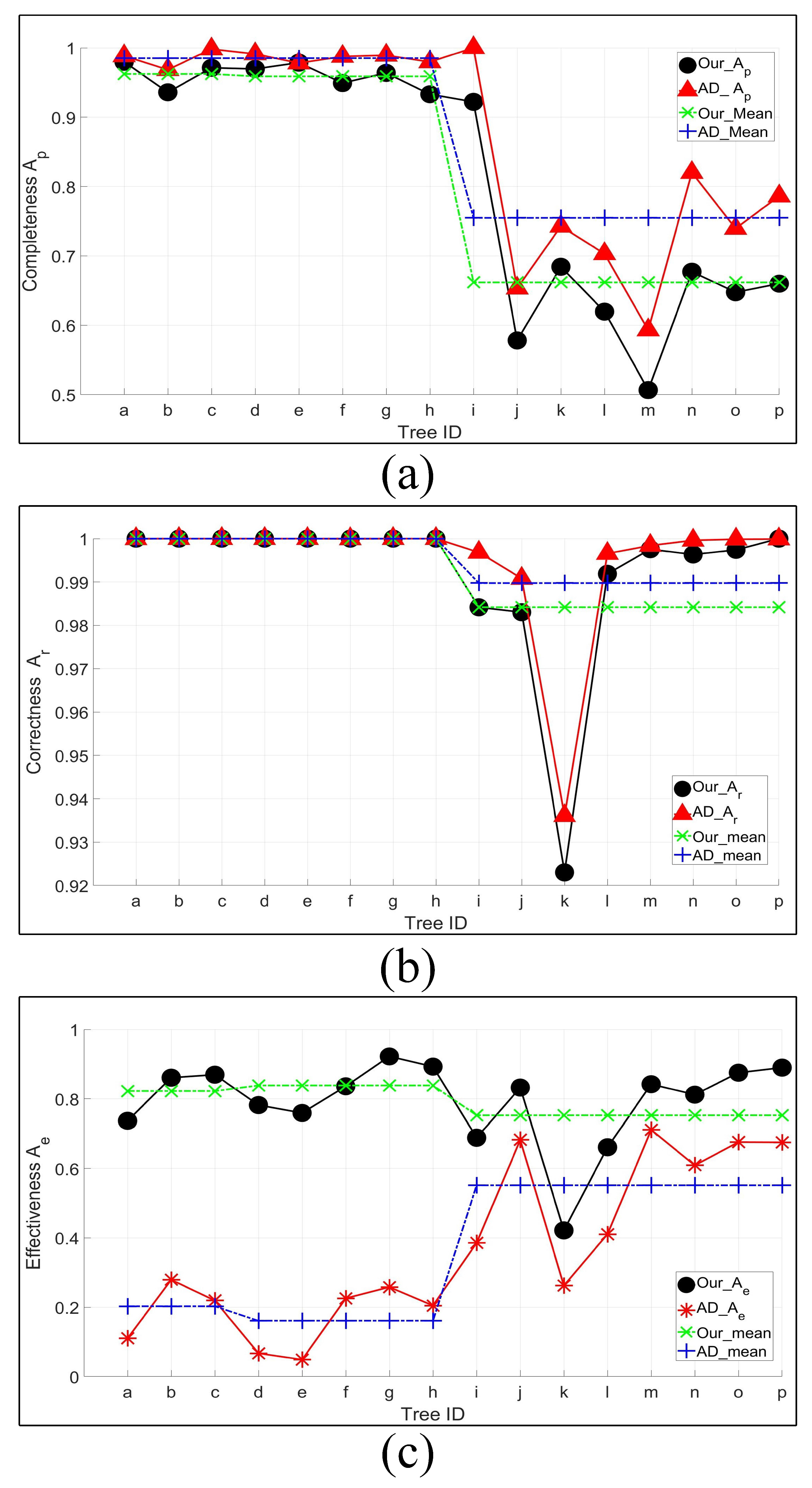
4.2. Quantitative Analysis

To evaluate our extraction quantitatively, we first compute the ratio between the number of points in input data and skeleton in Table 1.
We provide three metrics to evaluate our errors quantitatively. As shown in Figure 8a, if extracted skeletons are far from stems, those skeletons have low accuracy. As defined in Equation (6), the completeness A p shows how many points from the input data can be represent by our skeleton, and the correctness A r shows how many points from skeleton are correct, that is, spatially close to input data.
A p = 1 n · i = 1 n δ p i o , p j r , A r = 1 m · j = 1 m δ p i o , p j r
In Equation (6), p i o P o , p j r P r , where P o = { p 1 o , p 1 o , . . . . . . , p n o } shows input data and P r = { p 1 r , p 1 r , . . . . . . , p m r } shows result skeleton. n and m are the number of points in input data and result skeleton. δ p i o , p j r is a binary function. If the Euclidean distance between p i o and p j r is less than T, that is, 0.2 m, δ is 1, otherwise, it turns out to be 0.
As shown in Figure 8b, we do not want too many redundant points for the skeleton extraction. The effectiveness A e is defined as in Equation (7), which shows how many points that are effective in the skeleton representation. We want high completeness, correctness, and effectiveness in the algorithm, as shown in Figure 8c.
A e = 1 j = 1 m Card I m , I = i | δ p i o , p j r = 1 .
In Equation (7), Card I is the number of unique elements in the set I . Effectiveness is to measure the ratio of non-redundant points. If there is no redundant point, A e will be 1.
The comparison of the accuracy is shown in Figure 9. The average completeness, correctness and effectiveness of the proposed skeleton approach and AD is 81.10% and 86.99%, 99.21% and 99.49%, 79.26% and 36.41%, respectively. AD_mean and Our_mean are in shown Figure 9, which show the average accuracy of each metric on each type of trees. Although our completeness is less than AD, our correctness is close to AD and we have a much higher effectiveness than AD. This means that we have superiority in the subsequent modeling process, which is also proved by the fact that we have only used 5.82% of the input tree points, while AD is up to 40.19% of the original points.
The proposed skeleton extraction is fundamental to 3D modeling and structure study (e.g., breeding and phenotypic learning), which provides optimal tree branch information. Our key codes and experimental data have been submitted to Github (https://github.com/lostagex/skeleton_extraction, accessed on 22 September 2021) for readers refereed in the future comparison.

4.3. Discussion

In order to conduct the sensitive analysis of parameter setting, we divide our parameters into three types, namely the empirical setting, users’ demand-dependent and tree scene-dependent. In the aspect of setting the number of points in a neighboring set, the radius of the neighbor region, and the minimum length of a path, we have tried different discrete parameters, that is, 10–50 points for the neighboring set, 0.01–0.1 for the neighboring region and 1–10 points for the path length. We found that when we set 30, 0.05, and 5 for the above-mentioned parameters, we achieve high quality for all 16 tree sets in 3 tree species. Users’ demand-dependent parameters include λ and the number of iterations for the path smoothness. If users want skeletons to keep sharp, we suggest a small λ and fewer iterations, otherwise, users will achieve branches with rounded corners.
It is a little difficult to set ϕ for candidate point extraction, c and α for dynamic path calculation, and δ for the evaluation, because those rely on the input scene. If users want more candidate points, we suggest a small ϕ at the risk of reducing the subsequent skeleton extraction effectiveness. The setting of ϕ relies on the point density and trunk thickness of input trees. The setting of c and α is used to tune the weights of the data term and smoothness term. A tree set containing plentiful candidate points should pay more attention to the data term, which means a large c and a small α . However, if trees have fewer candidate points, we can only rely on the smoothness term to find the optimal path for the current branch, that is, a small c and a large α , otherwise, we will find a branch passing through all candidate points. In the quantitative analysis, we set the threshold as 0.2 m for the binary function δ . If one wants to use more rigorous estimation, he or she can tune a smaller threshold. Skeleton points that are further than this threshold will be regarded as false results.
We use fixed parameters in the skeleton extraction which is easy in the parameter setting. However, our completeness in Platanus acerifolia is not high, which means that different species require different parameter configurations. Because our extraction highly depends on the achieved candidate points. There are two potential improvements for constructing skeletons. Firstly, we can provide more rotation data for the candidate point extraction. Secondly, for thin branches containing much fewer points, we have to add weights of those points in the dynamic path optimization.
The proposed extraction framework works well on broadleaf trees. In the case of conifer species, we extract stems under crowns effectively. If users want to achieve the second branching order of trees, they are required to point out ending points manually as much as possible. Our extraction results highly depend on the candidate point detection, which is based on the ratio of points from a branch. Therefore, in the case of young trees, that is, DBH (diameter at breast height) is less than 10 cm, we ask users to spend more time in the scanning. The qualitative evaluation of the accuracy of the branch angle at each branching point is based on the path angle pointing to ending points. As shown in Figure 5, our growth trend of each branch is the same as the visually obtained branches.
As shown in Figure 9, the performances of AD and the proposed method seem possibly essentially different between Tree IDs. Because the skeleton extraction performance is related to the height of trees and the scanning completeness. Hence, there is a big difference between Prunus serrulate/Ginkgo biloba (height < 10 m) and Platanus acerifolia (height > 20 m). Experiments show that the proposed method is effectively utilized in the extraction of branches when trees are less than 10 m. Besides, our work keeps high performance in the extraction of skeleton points from the first and second branching order. In terms of Platanus acerifolia, we found that it is difficult to keep high completeness in the skeleton extraction from the third or fourth branching order when keeping high effectiveness.

5. Conclusions

This work proposed a framework to achieve skeletons from portable scanning point clouds. We proposed four main steps, including candidate points extraction, dynamic path optimization, points interpolation, and path refinement & smoothness. In the proposed approach, candidate points are extracted to reduce calculation for the subsequent path optimization. The path cost is minimized by the dynamic programming technique to obtain the global optimization. Later, points are interpolated between candidate points to complete paths, and false paths are removed. True paths are smoothed to be presented as the tree skeleton. Experiments show that the proposed work succeeded in extracting skeleton from various trees. The achieved visual quality of our skeleton extraction is high. All points from the first branching order were detected. The extraction of points from the second branching order depends on the thickness. The accuracy evaluation shows that our method obtained good completeness and correctness of 81.10% and 99.21%. At the same time, we achieved high effectiveness of 79.26%, which is better than the compared method at 36.41%. Only 5.82% of the input tree points were used in the skeleton representation. It can also be concluded that the portable laser scanning system works effectively in 3D structure analysis, which is flexible in capturing space information.
Although we were able to effectively achieve the branch structure by the proposed tree skeleton extraction framework, our skeletons are highly reliant on the results of candidate point extraction. It is difficult to find the third branching order of trees, which are tiny in PLS point clouds, that is, branches containing 2.3 points only. Future work will focus on three parts: first, the improvement of the extraction efficiency to apply the approach to sparse data, such as airborne laser scanning point clouds, for obtaining large-scale forest branches; and second, the analysis of the branch structure of different trees for their phenotyping study and breeding.

Author Contributions

Conceptualization, S.X. (Sheng Xu); Methodology, S.X. (Sheng Xu) and S.X. (Shanshan Xu); Writing—original draft preparation, X.L. and J.Y.; Writing—review and editing J.Y. All authors have read and agreed to the published version of the manuscript.

Funding

This work was supported in part by the National Natural Science Foundation of China (Grant No.62102184), in part by the Natural Science Foundation of Jiangsu Province (Grant No.BK20200784), in part by China Postdoctoral Science Foundation (Grant No.2019M661852) and in party by the National Key Research and Development Program of China (Grant No.2019YFD1100404).

Institutional Review Board Statement

Not applicable.

Informed Consent Statement

Not applicable.

Data Availability Statement

Not applicable.

Conflicts of Interest

The authors declare no conflict of interest.

References

  1. Yun, T.; Jiang, K.; Li, G.; Eichhorn, M.P.; Fan, J.; Liu, F.; Chen, B.; An, F.; Cao, L. Individual tree crown segmentation from airborne LiDAR data using a novel Gaussian filter and energy function minimization-based approach. Remote Sens. Environ. 2021, 256, 112307. [Google Scholar] [CrossRef]
  2. Yun, T.; Cao, L.; An, F.; Chen, B.; Xue, L.; Li, W.; Pincebourde, S.; Smith, M.J.; Eichhorn, M.P. Simulation of multi-platform LiDAR for assessing total leaf area in tree crowns. Agric. For. Meteorol. 2019, 276, 107610. [Google Scholar] [CrossRef]
  3. Hu, C.; Pan, Z.; Zhong, T. Leaf and wood separation of poplar seedlings combining locally convex connected patches and K-means++ clustering from terrestrial laser scanning data. J. Appl. Remote Sens. 2020, 14, 1. [Google Scholar] [CrossRef]
  4. Li, Q.; Yuan, P.; Liu, X.; Zhou, H. Street tree segmentation from mobile laser scanning data. Int. J. Remote. Sens. 2020, 41, 7145–7162. [Google Scholar] [CrossRef]
  5. Xia, S.; Wang, R. Semiautomatic construction of 2-D façade footprints from mobile LIDAR data. IEEE Trans. Geosci. Remote Sens. 2019, 57, 4005–4020. [Google Scholar] [CrossRef]
  6. Wang, D.; Hollaus, M.; Puttonen, E.; Pfeifer, N. Automatic and self-adaptive stem reconstruction in landslide-affected forests. Remote Sens. 2016, 8, 974. [Google Scholar] [CrossRef] [Green Version]
  7. Zhang, W.; Wan, P.; Wang, T.; Cai, S.; Chen, Y.; Jin, X.; Yan, G. A novel approach for the detection of standing tree stems from plot-level terrestrial laser scanning data. Remote Sens. 2019, 11, 211. [Google Scholar] [CrossRef] [Green Version]
  8. Xu, S.; Zhou, K.; Sun, Y.; Yun, T. Separation of Wood and Foliage for Trees from Ground Point Clouds using a Novel Least-cost Path Model. IEEE J. Sel. Top. Appl. Earth Obs. Remote Sens. 2021, 14, 6414–6425. [Google Scholar] [CrossRef]
  9. Fu, L.; Li, Z.; Ye, Q.; Yin, H.; Liu, Q.; Chen, X.; Fan, X.; Yang, W.; Yang, G. Learning robust discriminant subspace based on joint L2, p-and L2, s-Norm distance metrics. IEEE Trans. Neural Netw. Learn. Syst. 2020. [Google Scholar] [CrossRef] [PubMed]
  10. Ye, Q.; Huang, P.; Zhang, Z.; Zheng, Y.; Fu, L.; Yang, W. Multiview Learning With Robust Double-Sided Twin SVM. IEEE Trans. Cybern. 2021. [Google Scholar] [CrossRef] [PubMed]
  11. Gaillard, M.; Miao, C.; Schnable, J.; Benes, B. Sorghum segmentation by skeleton extraction. In Computer Vision–ECCV 2020 Workshops; Lecture Notes in Computer Science; Springer: Cham, Switzerland, 2020; Volume 12540. [Google Scholar] [CrossRef]
  12. Zhang, C.; Yang, G.; Jiang, Y.; Xu, B.; Li, X.; Zhu, Y.; Lei, L.; Chen, R.; Dong, Z.; Yang, H. Apple tree branch information extraction from terrestrial laser scanning and backpack-lidar. Remote Sens. 2020, 12, 3592. [Google Scholar] [CrossRef]
  13. Xu, H.; Gossett, N.; Chen, B. Knowledge and heuristic-based modeling of laser-scanned trees. ACM Trans. Graph. (TOG) 2007, 26, 19-es. [Google Scholar] [CrossRef]
  14. Bucksch, A.; Lindenbergh, R. CAMPINO—A skeletonization method for point cloud processing. ISPRS J. Photogramm. Remote Sens. 2008, 63, 115–127. [Google Scholar] [CrossRef]
  15. Livny, Y.; Yan, F.; Olson, M.; Chen, B.; Zhang, H.; El-Sana, J. Automatic reconstruction of tree skeletal structures from point clouds. In ACM SIGGRAPH Asia 2010 Papers; Association for Computing Machinery: New York, NY, USA, 2010; pp. 1–8. [Google Scholar] [CrossRef] [Green Version]
  16. Wang, Z.; Zhang, L.; Fang, T.; Mathiopoulos, P.T.; Qu, H.; Chen, D.; Wang, Y. A structure-aware global optimization method for reconstructing 3-D tree models from terrestrial laser scanning data. IEEE Trans. Geosci. Remote Sens. 2014, 52, 5653–5669. [Google Scholar] [CrossRef]
  17. Du, S.; Lindenbergh, R.; Ledoux, H.; Stoter, J.; Nan, L. AdTree: Accurate, detailed, and automatic modelling of laser-scanned trees. Remote Sens. 2019, 11, 2074. [Google Scholar] [CrossRef] [Green Version]
Figure 1. Flowchart of the proposed skeleton extraction approach.
Remotesensing 14 00094 g001
Figure 2. Candidate point extraction. (a) Split of input data into slices. (b) Examples of candidate point extraction results.
Remotesensing 14 00094 g002
Figure 3. Example of searching optimal path for the point p 7 .
Remotesensing 14 00094 g003
Figure 4. Results of the point interpolation.
Remotesensing 14 00094 g004
Figure 5. Results of the path refinement and smoothness. (a) Classification of the ending points and branching points. (b) Refinement results. (c) Smoothness results.
Remotesensing 14 00094 g005
Figure 6. Results of the skeleton extraction. For each subfigure from (ap), the first row shows the input data, the second row shows the result of AD [17], and the last row shows our results.
Remotesensing 14 00094 g006
Figure 7. Comparison of the skeleton extraction with AD [17].
Remotesensing 14 00094 g007
Figure 8. Evaluation of the skeleton extraction. (a) Low accuracy. (b) Low effectiveness. (c) Desired results.
Remotesensing 14 00094 g008
Figure 9. Quantitative comparison of our method and AD. (a) Completeness. (b) Correctness. (c) Effectiveness.
Remotesensing 14 00094 g009
Table 1. Data information of skeleton extraction.
IDH (m)SPOur_PAD_PAD_RatioOur_Ratio
a7.80122,520156625,9301.1510.070
b8.42171,220198279,7831.1200.028
c7.621127,8681620133,9791.0480.013
d9.432413,249276337,8410.0920.007
e9.562945,333264835,5850.0380.003
f8.202632,514189128,2430.0450.003
g7.752789,197279634,5050.0440.004
h7.412614,486216835,9700.0590.004
i18.58331,977631127,7010.8660.197
j21.493424,61810,63945,4310.1070.025
k21.0131,175,513848534,9280.0300.007
l21.0931,531,635912238,2480.0250.006
m23.1531,528,38210,72240,9530.0270.007
n24.68316,407738121,8181.3300.450
o25.42395,923960940,1070.4180.100
p23.6131,316,13611,41443,3610.0330.009
The first column ‘ID’ corresponds to the result in Figure 6. The second column ‘H’ shows the elevation of each tree. The third column ‘S’ shows the specie of each tree, including #1 Prunus serrulata, #2 Ginkgo biloba L. and #3 Platanus acerifolia. The fourth column ‘P’ shows the number of input points. The fifth and sixth columns show the number of points in the skeleton achieved from our method and AD, respectively. The last two columns show the ratio of points in the skeleton and input data achieved by our method and AD, respectively.
Publisher’s Note: MDPI stays neutral with regard to jurisdictional claims in published maps and institutional affiliations.

