Evaluation of Surface Reflectance Products Based on Optimized 6S Model Using Synchronous In Situ Measurements

Abstract

Surface reflectance (SR) estimation is the most essential preprocessing step for multi-sensor remote sensing inversion of geophysical parameters. Therefore, accurate and stable atmospheric correction is particularly important, which is the premise and basis of the quantitative application of remote sensing. It can also be used to directly compare different images and sensors. The Landsat-8 Operational Land Imager (OLI) and Sentinel-2 Multi-Spectral Instrument (MSI) surface reflectance products are publicly available and demonstrate high accuracy. However, there is not enough validation using synchronous spectral measurements over China’s land surface. In this study, we utilized Moderate Resolution Imaging Spectroradiometer (MODIS) atmospheric products reconstructed by Categorical Boosting (CatBoost) and 30 m ASTER Global Digital Elevation Model (ASTER GDEM) data to adjust the relevant parameters to optimize the Second Simulation of Satellite Signal in the Solar Spectrum (6S) model. The accuracy of surface reflectance products obtained from the optimized 6S model was compared with that of the original 6S model and the most commonly used Fast Line-of-sight Atmospheric Analysis of Spectral Hypercubes (FLAASH) model. Surface reflectance products were validated and evaluated with synchronous in situ measurements from 16 sites located in five provinces of China: Fujian, Gansu, Jiangxi, Hunan, and Guangdong. Through the indirect and direct validation across two sensors and three methods, it provides evidence that the synchronous measurements have the higher and more reliable validation accuracy. The results of the validation indicated that, for Landsat-8 OLI and Sentinel-2 MSI SR products, the overall root mean square error (RMSE) calculated results of optimized 6S, original 6S and FLAASH across all spectral bands were 0.0295, 0.0378, 0.0345, and 0.0313, 0.0450, 0.0380, respectively. R² values reached 0.9513, 0.9254, 0.9316 and 0.9377, 0.8822, 0.9122 respectively. Compared with the original 6S model and FLAASH model, the mean percent absolute error (MPAE) of the optimized 6S model was reduced by 32.20% and 15.86% for Landsat-8 OLI, respectively. On the other, for the Sentinel-2 MSI SR product, the MPAE value was reduced by 33.56% and 33.32%. For the two kinds of data, the accuracy of each band was improved to varying extents by the optimized 6S model with the auxiliary data. These findings support the hypothesis that reliable auxiliary data are helpful in reducing the influence of the atmosphere on images and restoring reality as much as is feasible.

1. Introduction

Surface reflectance is the most basic remote sensing parameter in the solar reflectance spectral bands (visible spectrum and infrared spectrum), and is an important input parameter to obtain leaf area index, vegetation index, burn area identification, water quality parameters, and aerosol optical depth (AOD) [1]. Atmospheric correction is the most important step in surface reflectance inversion and its purpose is to obtain the true surface reflectance data of ground objects [2]. In 1997, Vermote developed the 6S model, an open-source code [3]. Due to its advantages of fast calculation and high accuracy, the 6S model is used in radiation calibration, AOD retrieval, surface albedo research, and atmospheric correction [4,5,6]. The 6S model can simulate a more realistic surface, atmospheric, and observation environment. The wavelength of the spectral integral is increased from 5 nm to 2.5 nm, taking into account the altitude of the ground target, the condition of the non-Lambert plane, and the new absorbed gases (CH₄, N₂O, CO). The 6S model is suitable for the spectral band from 0.25 µm to 4.0 µm. The art approximation algorithm and Successive Orders of Scattering (SOS) algorithm have been introduced to improve the calculation accuracy of Rayleigh and aerosol scattering. Due to the radiative transfer theory, the 6S model can guarantee the correction accuracy without limitation by the research characteristics and target types, thus its use is more widely applicable.

Many scholars have obtained reflectance products by atmospheric correction based on the 6S model. Giannis et al. used the 6S model, FLAASH model, and Dark Object Subtraction (DOS) model to carry out an atmospheric correction on Sentinel-2 high-resolution image [7]. Eric et al. used the 6S model to analyze the performance of the Landsat-8 OLI SR product at Aerosol Robotic Network (AERONET) sites and estimate atmospheric parameters from the Landsat itself [8]. Wang et al. developed a MODIS-based per-pixel atmospheric correction procedure combined with the 6S model [9]. Neil used the 6S model to conduct atmospheric correction on Sentinel-2, Landsat-7/8 data throughout the Australian region to obtain SR products and establish linear relationships among the three data sources, and compare them with the Harmonized Landsat-8 Sentinel-2 Product (HLS) [10]. A method based on the 6S model without considering aerosol particles and atmospheric gas information was proposed and applied by using 2000–2018 Landsat-5/7/8 data [11]. Kyeong-sang Lee improved the 6S look-up method by using the minimum curvature surface method to obtain surface reflectance and compared it with the surface reflectance calculated by using 6S only [12].

Previous researchers have used different methods to validate the accuracy of SR products. Some studies also analyzed the accuracy of the Landsat Ecosystem Disturbance Adaptive Processing System (LEDAPS) algorithm and compared it to AERONET sites, MODIS SR products, and rigorous radiative transfer [13,14,15,16,17]. Maiersperger et al. compared LEDAPS surface reflectance products using AERONET observations, field spectroscopy, and MODIS SR data. The results confirm the success of LEDAPS SR inversion on long-wavelength in vegetation covered areas. In the case of shorter wavelength and sparseness, the reliability of a vegetated area has shown to be low [16]. Eric et al. used three different methods to validate the Landsat-8 OLI SR product indirectly: (i) AERONET data; (ii) MODIS SR products; and (iii) the measurements of 5 sites. The results clearly showed an improvement of the Landsat-8 OLI surface reflectance product over the ad-hoc Landsat 5/7 LEDAPS product [8]. Moe et al. validated the Landsat-8 OLI Level-2 reflectance products with near-synchronous measurements from 13 test sites in the United States, Brazil, and elsewhere. The results consistently showed similarities between OLI Level-2 SR products and ground measured data [18]. Recently, a study using in situ measurements has shown that the Landsat-8 OLI Level-2 improved surface reflectance product over all spectral bands in common with the Landsat-7 ETM plus Level-2 data [19].

Accurate atmospheric parameters are crucial for transferring top-of-atmosphere (TOA) radiance or reflectance to surface reflectance products [20]. It is challenging to use fixed atmospheric parameters or estimated atmospheric parameters from Landsat images as input parameters to the 6S model, due to the variability of the atmospheric environment and the low spectral resolution of the image [9]. The elevation parameters mostly use the Global Multi-resolution Terrain Elevation Data (GMTED) 2010 data with low spatial resolution. The precision of the parameters may need to be improved. The method and data in the references are relatively single, and the universality of the method may not be considered. Most validation efforts relied on an indirect comparison with corresponding data, such as the MODIS SR products that were simultaneously acquired by a well-calibrated sensor [9,21]; however, comparisons with these data are limited due to its much lower spatial resolution and AERONET does not have estimated values of surface reflectance. In addition, there are relatively few relevant studies on validating remote sensing surface reflectance by using a large number of synchronous measurement spectral data. In terms of data sources, the above studies mainly use a single data source, in particular, the differences between sensors are rarely involved in using measurements. In terms of the study area, although there are surface synchronous survey verification methods in the literature, reflectance retrieval and validation of synchronous in situ measurements in large areas of China are not involved at present. The studies are less concerned about whether the reflectance of the same ground object is different due to different geographical locations or surrounding environments.

In this study, we utilized MODIS atmospheric products reconstructed by CatBoost and 30 m ASTER GDEM data to adjust the relevant parameters to optimize the 6S model. Higher precision parameters were used for the 6S model. We applied the optimized 6S model to Landsat-8 OLI and Sentinel-2 MSI data sources and compared the results with the original 6S and FLAASH model results using a large number of synchronous measurements. It is important to emphasize that the traditional synchronous ground measurement method is the most direct and best validation method to obtain the surface reflectance of the objects. Multi-type synchronous surface spectral measurement data in the large-scale area were applied for validation of the surface reflectance of satellite images, a wide geographic distribution mainly takes into account different cover types and atmospheric conditions. Most importantly, the deficiency of indirect verification between sensors can be avoided.

The structure of the paper is as follows. The first part provides an introduction to the study; the second part details the data used in the study; the third part outlines the methods; the fourth section demonstrates how the measured data used in validating and evaluating the accuracy of surface reflectance products of different sensors; and the fifth and sixth sections present the discussion and conclusion.

2. Data

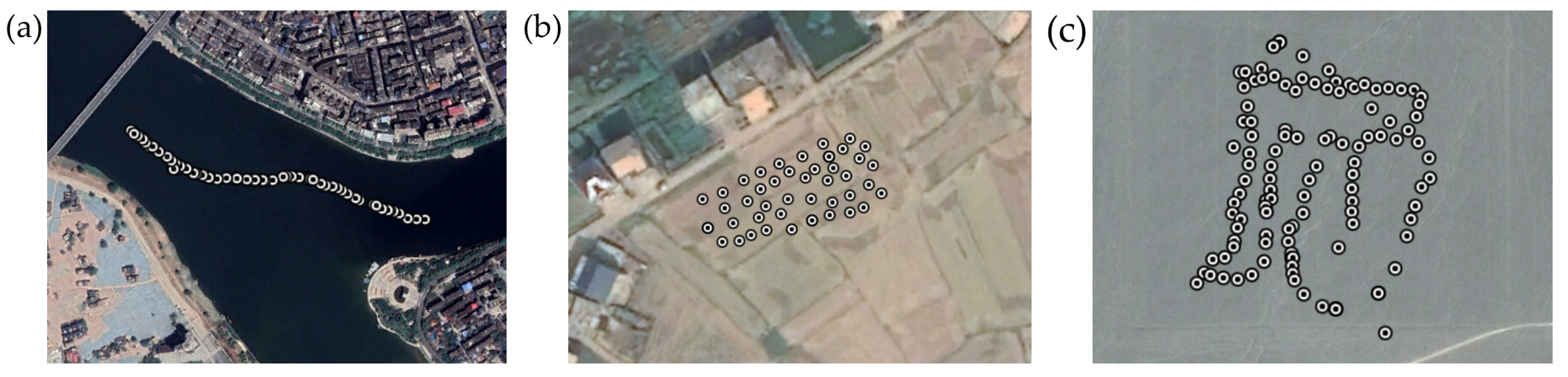
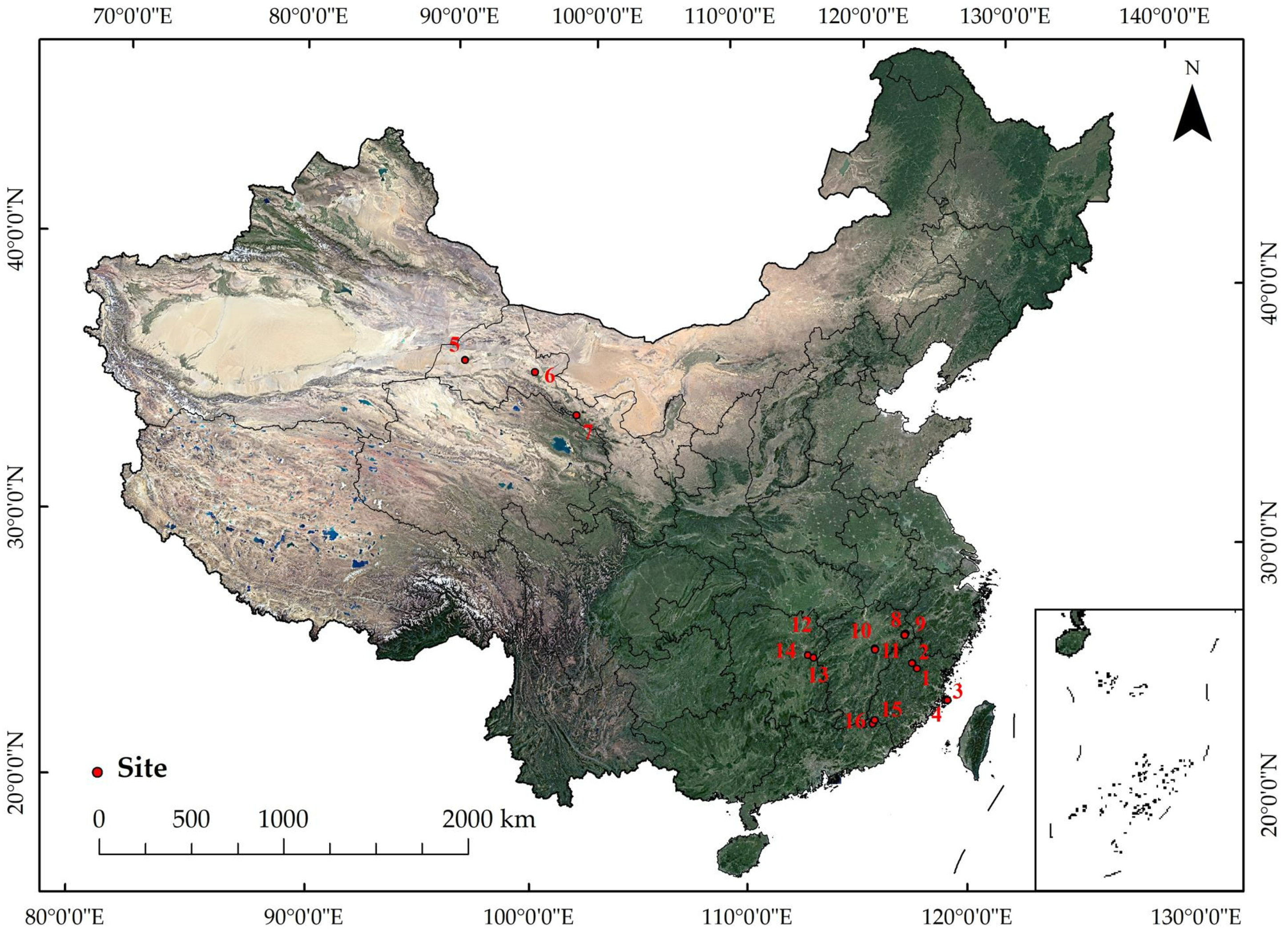
2.1. In Situ Measurements

In this study, we validated and evaluated the SR products of different sensors using in situ measurements. This part describes the distributions and related information of the in situ measurements synchronized with Landsat-8 overpass time. We measured spectral data from more than 20 sites, but because of the weather and other reasons, we ruled out some sites with questionable data. Through our efforts, we obtained optimal spectral data from 16 sites of five provinces in 2019: Fujian, Jiangxi, Guangdong, Hunan, and Gansu.

Synchronous measurements were collected by on-site personnel (4–10) using the Analytical Spectral Devices (ASD) FieldSpec4 Hi-Res Surface High Spectroradiometer (350–2500 nm). The Spectroradiometer is equipped with a fiber-optic probe to retrieve spectral characteristics of ground sites in this study. The specific procedures for collecting spectral data are as follows:

(1)

Place the white board around the sample and make sure that the white board is in the same level position as the sample surface. The operator faces the sun and makes the optical fiber is aligned vertically with the white board to determine the optical fiber sampling height.

(2)

Optimize the Spectroradiometer. Re-optimize every 15–20 min or when lighting conditions and environmental conditions change significantly. Each time the target is changed, the spectroradiometer is re-optimized.

(3)

After the optimization, the optical fiber is still vertically aligned with the whiteboard, and the DN value of reflected light is collected. Then the DN value of the sample will be collected and compared with the average DN value of the whiteboard, and the reflectance of the sample is calculated.

(4)

The optical fiber aims at the sample and makes the relative reflectance curve of the sample display stably on the interface.

(5)

The current spectral curve is stored. Five radiance spectra curves as a group are collected for each point, and dozens or even hundreds of groups of data are collected for each site. These results are then averaged (after manual removal of spurious spectra) by ViewSpecPro software to retain the optimal spectral curve and achieve a representative radiance spectrum.

(6)

The native spectral resolution across the full range (i.e., 3 nm in the VNIR and 8 nm in the SWIR) is internally resampled to 1 nm for the output spectra.

The overpass time and location of the next Landsat-8 OLI were calculated according to that of the previous large number of Landsat-8 OLI. Survey personnel arrived at the crossing site one hour in advance to perform a series of preparatory work, such as ASD warm-up of instruments and calibration of the white board. In general, the measurement started half an hour before the satellite crossed the area. Sample points were evenly selected to collect data and mark coordinates in the measurement area, the geolocation of the sample points was established using a GPS kit with a positional accuracy of approximately 1 m. The marked sample points were about 30 m apart. Synchronous measurements were obtained with vegetation, water, and bare land sites, in which their surface area was large and homogeneous. Figure 1 shows the sample points of route maps for 3 representative ground features.

According to the above protocols, we completed these massive synchronous in situ measurements. The distribution of all measured sites (Figure 2) and field measurement scenario of each site (Figure 3) are as follows:

(1)

Fujian: Rice at heading stage and water in Nanping; sand beach and water in Pingtan.

(2)

Gansu: Two Gobi Desert sites in Dunhuang and Jiayuguan; wheat in Zhangye.

(3)

Jiangxi: River water, mature rice in Shangrao; rice at heading stage and mature rice in Fuzhou.

(4)

Hunan: Rice stubble, grass, and Xiangjiang river in Zhuzhou.

(5)

Guangdong: Mature rice and lake water in Meizhou.

Sites 1–4 were located in Fujian Province. Site 1 includes a sample of vegetation in Nanping; the growth of rice was relatively homogeneous when collecting data. Sites 2 and 4 were water located in Nanping and Pingtan, respectively. The land cover of Site 3, in Pingtan, was sand beach sand. At this site, the measured sand was moist because of its being constantly buffeted by the sea currents.

Sites 5–7 were located in Gansu Province. Both sites 5 and 6 were the Gobi. The texture at site 5, radiation correction field in Dunhuang, was relatively uniform. Site 6 was located at Gobi in Jiayuguan, surrounded by the endless Gobi with flat terrain, uniform texture, and no other disturbance land types. Site 7 was wheat in Zhangye, the representative crop of northern China. The wheat was ripe at the time of measurement.

Sites 8–11 were located in Jiangxi Province. Site 8 was the water in Shangrao, which was generally deep and of good quality. We specially chartered a boat to measure the reflectance of the water in the deep area. Site 9 was the rice whose leaves were already yellowish and about to mature in Shangrao. Site 10 and Site 11 were rice with a different growth period in Fuzhou, in which the spectral responses of different maturity vegetation were compared.

Sites 12–14 were located in Zhuzhou, Hunan Province. Site 12 was at rice stubble cover in which the rice was harvested. Site 13 was grass, which was green, evenly distributed. Sites 14 was at the Xiangjiang river, which covered the shallow and deep water zone.

Sites 15–16 were located in Meizhou, Guangdong province. Site 15 was the location of rice; the land surface type of the sample plot was a large area of mature rice about a few acres in size. Sites 16 was the lake water with different depths.

The satellite overpass time, measurement time, and weather conditions of each site were shown in

Table 1. Ground truth sites data in 2019 used in this study.

Site of Samples		City/ Province	Overpass Time		Cloud Cover (%)	Measured Time
Code	Land Type		Landsat-8	Sentinel-2
1	Rice at Heading Stage	Nanping/ Fujian	10: 38/13/09	10: 35/11/09	24.51/21.03	10: 12–10: 57/13/09
2	Water					14: 02–14: 15/13/09
3	Sand Beach	Pingtan/ Fujian	10: 26/15/09	no data	17.46/no	10: 17–10: 37/15/09
4	Water					12: 22–12: 43/15/09
5	Gobi Desert	Dunhuang/ Gansu	12: 20/20/09	12: 27/20/09	0.46/1.08	11: 12–13: 45/20/09
6	Gobi Desert		12: 07/22/09	12: 15/21/09	2.28/80.34	11: 50–12: 58/22/09
7	Wheat	Zhangye/ Gansu	11: 56/24/09	no data	4.87/no	11: 49–12: 20/24/09
8	Water	Shangrao/ Jiangxi	10: 38/29/09	10: 45/29/09	1.97/1.33	10: 35–11: 08/29/09
9	Mature Rice					12: 27–12: 55/29/09
10	Rice at Heading Stage	Fuzhou/ Jiangxi	10: 44/06/10	10: 45/04/10	44.65/0.31	12: 13–12: 38/06/10
11	Mature Rice					12: 40–12: 54/06/10
12	Rice Stubble	Zhuzhou/ Hunan	10: 56/20/10	11: 07/20/10	5.37/6.00	10: 48–11: 09/20/10
13	Grass					11: 11–11: 22/20/10
14	Xiangjiang River					13: 12–13: 38/20/10
15	Mature Rice	Meizhou/ Guangdong	10: 45/22/10	10: 47/19/10	9.40/5.03	10: 28–10: 59/22/10
16	Lake Water					12: 47–13: 12/22/10

.

2.2. Landsat-8 OLI and Sentinel-2 MSI

Landsat-8 was launched in February 2013 and its orbit was 705 km [22]. The imaging swath was 185 km and the revisit period was 16 days. The Landsat-8 OLI had seven multi-spectral reflectance bands. Collection 2 was publicly released in mid-2020. Its biggest features included sensor radiometric calibration and updated geometric accuracy. Landsat-8 Collection 2 Level-1 data was tested in this study. Sentinel-2 carries MSI [23]. Sentinel-2A and Sentinel-2B were launched in June 2015 and March 2017, respectively, into circular sun-synchronous 786 km orbits [24]. The data provide a 290 km imaging swath, and the revisit period was 10 days of each Sentinel-2 sensor and 5 days when combined.

Due to these different orbits and swath widths, OLI and MSI may detect certain targets on the same day. The accuracy of the SR products was validated using synchronous measurements during the Landsat-8 overpass. The overpass time of Sentinel-2 was close to that of Landsat-8, but not be fully synchronous with Landsat-8, and most of the objects observed were land objects with no mobility. We can assume that the surface does not change as the two satellites overpass.

Selecting the common and similar bands for experiments can avoid or weaken the differences between the data of different sensors to a certain extent (

Table 2. Approximate equivalent bands of Landsat-8 OLI and Sentinel-2 MSI in this study.

Landsat-8 OLI			Sentinel-2 MSI
Band	Resolution (m)	Wavelength (nm)	Band	Resolution (m)	Wavelength (nm)
B1 (Coastal)	30	430–450	B1 (Coastal)	60	433–453
B2 (Blue)	30	450–515	B2 (Blue)	10	458–523
B3 (Green)	30	525–600	B3 (Green)	10	543–578
B4 (Red)	30	630–680	B4 (Red)	10	650–680
B5 (NIR)	30	845–885	B8 (NIR)	10	785–900
B6 (SWIR-1)	30	1560–1660	B11 (SWIR-1)	20	1565–1655
B7 (SWIR-2)	30	2100–2300	B12(SWIR-2)	20	2100–2280

). For Sentinel-2 MSI, band 8, with a resolution of 10 m, was taken as the NIR band for comparison.

2.3. Auxiliary Data

The influence of the atmosphere on the reflectance band of Landsat mainly includes aerosol, water vapor, and ozone [25]. We used three MODIS atmospheric products to optimize atmospheric parameters—MOD04 AOD values at 550 nm [26], MOD05 water vapor [27], and MOD07 total ozone [28].

ASTER GDEM is a Global Digital Elevation data product. The DEM data are completed based on the observations of NASA’s new generation Earth observation satellite Terra. The data have a horizontal accuracy of 1 (about 30 m, 95% confidence) and an elevation accuracy of 20 m (95% confidence). The Shuttle Radar Topography Mission (SRTM) and meteorological data were used to reconstruct AOD.

3. Methods

3.1. Categorical Boosting(CatBoost)

The contribution of the atmosphere to remote sensor signal can exceed 80% [29], and the atmospheric component that interferes most is aerosol [30]. AOD is an important parameter to describe aerosol quantitatively [31]. However, there are several missing phenomena in MOD04 products. The mechanism for reconstructing the missing MOD04 products to obtain a more accurate AOD parameter is crucial for atmospheric correction results.

CatBoost is a gradient boosting decision tree framework [32] based on tree boosting. CatBoost’s combination of iterations based on weak regressors can produce the theoretical expectation of a strong regressor, the same as the eXtreme Gradient Boosting (XGBoost) [33] and Light Gradient Boosting Machine (LightGBM). In this method, the traditional gradient estimation method is replaced by order boosting, which improves the generalization ability of the model and accuracy, and reduces the probability of overfitting [34]. For a variety of tasks, CatBoost is superior to other decision tree methods [35]. It is especially fit for the regression problem with noisy data and a number of input features [36], which is our AOD reconstruction. In this study, the hyperparameters are fine-tuned by the Bayesian Optimization algorithm [37]. After training with AOD data observed by remote sensing, the missing AOD was reconstructed with meteorological variables, day of the year, and elevation as independent variables. We formularized this regression problem as:

$$\mathrm{AOD}~f\left(\mathrm{DOY},\mathrm{Elev},{\mathrm{Mete}}_{\mathrm{t}}\right)$$

(1)

where $\mathrm{DOY}$ is the day of the year (1–365/366), and $\mathrm{Elev}$ is the elevation, ${\mathrm{Mete}}_{\mathrm{t}}$ is the 17-variable meteorological matrix at current day $\mathrm{t}$. These data were provided by Yu Ding [38]. We used the reconstructed MOD04 (AOD) as the AOD parameter to input into the 6S model in the next section (Section 3.2).

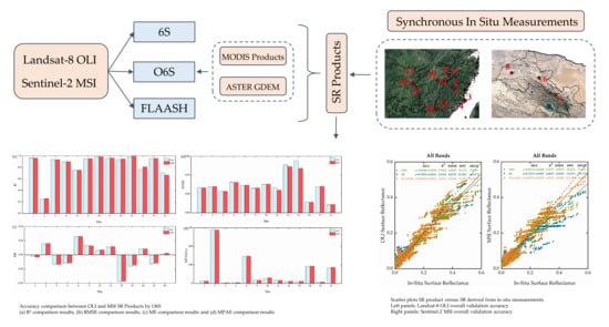
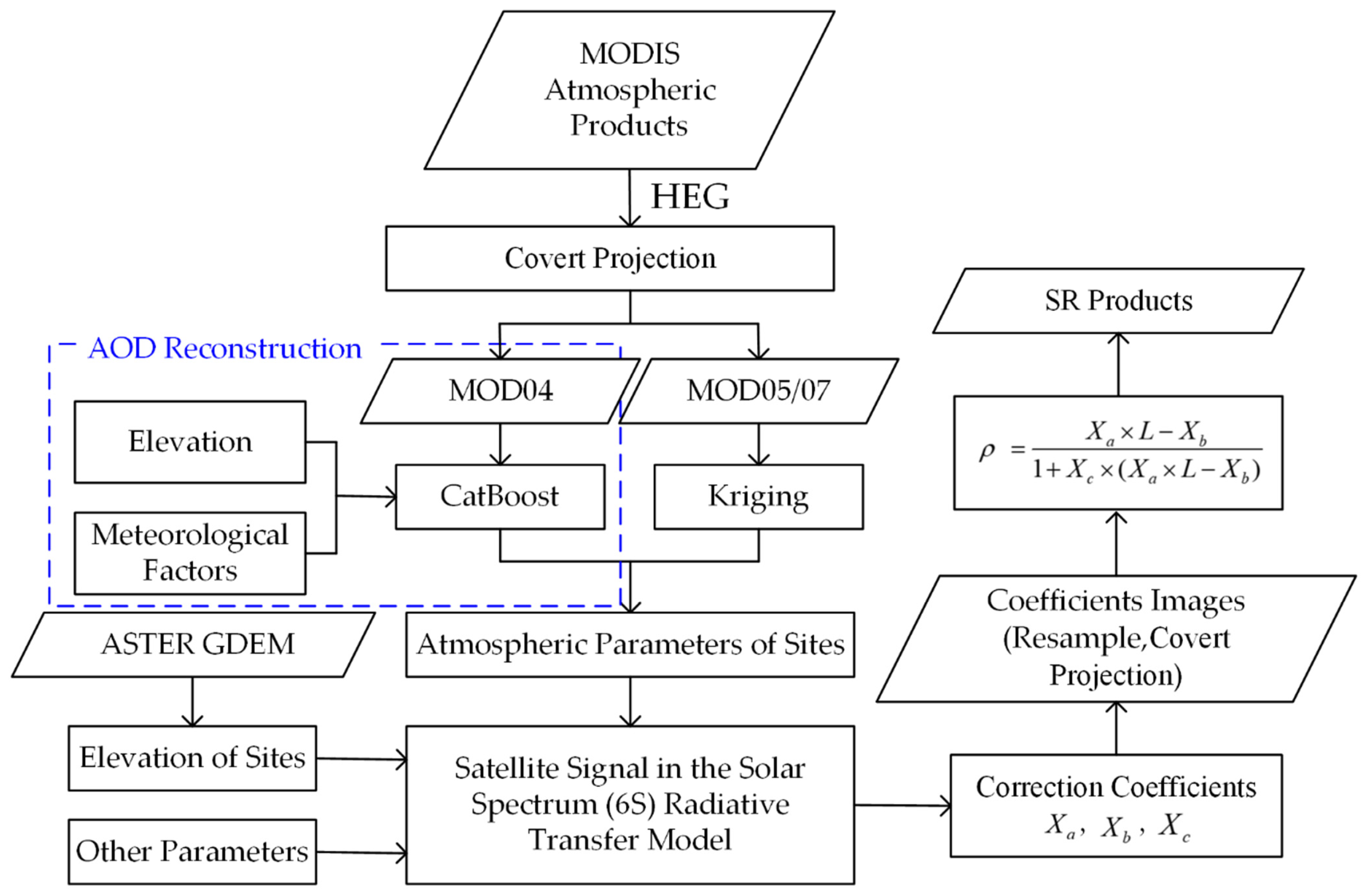
3.2. Optimized Second Simulation of the Satellite Signal in the Solar Spectrum (O6S)

The aim of atmospheric correction is to remove contributions to the atmosphere from the total signal measured by satellite sensors [39]. It plays a crucial role in converting apparent radiation measured by satellite sensors into surface reflectance [40]. The same method was used to correct the atmospheric top reflectance of OLI and MSI sensors to surface reflectance to reduce the bias that might occur if different methods were used. In this study, three methods were used to compare the accuracy: optimized 6S model with auxiliary data, original 6S model, and FLAASH model.

The 6S is an advanced radiative transfer code, which is not affected by the characteristics of the study area and target type [41]. According to the input parameters, the atmospheric correction coefficients ${\mathrm{X}}_{\mathrm{a}}$, ${\mathrm{X}}_{\mathrm{b}}$ and ${\mathrm{X}}_{\mathrm{c}}$ are calculated, using the 6S model, through these atmospheric correction coefficients and the TOA radiance ($\mathrm{L}$). The SR ($\mathsf{\rho }$) without atmospheric effects is obtained for each band. The calculation equation is as follows:

$$\mathsf{\rho }=\frac{{\mathrm{X}}_{\mathrm{a}}\times \mathrm{L}-{\mathrm{X}}_{\mathrm{b}}}{1+{\mathrm{X}}_{\mathrm{c}}\left({\mathrm{X}}_{\mathrm{a}}\times \mathrm{L}-{\mathrm{X}}_{\mathrm{c}}\right)}$$

(2)

The input parameters of the 6S model include geometric parameters, climate type, aerosol type, aerosol optical depth, target height, sensor height, spectral response function, and atmospheric correction mode. MODIS atmospheric products were used to optimize the climate type parameter (MOD05 water vapor products and MOD07 total ozone products) and AOD parameter (MOD04 AOD values at 550 nm reconstructed by CatBoost). DEM data were used to optimize the target elevation parameter. The procedures are as follows:

(1)

Convert the projection of MODIS atmospheric products (MDO04, MOD05, and MOD07) by HEG software.

(2)

The invalid values of the MODIS atmospheric products obtained in step (1) are reconstructed by the CatBoost (MOD04 AOD values at 550 nm) and Kriging (MOD05 water vapor products and MOD07 total ozone products) method.

(3)

Use the reconstructed MODIS atmospheric products, DEM, and other input parameters, the 6S model calculates atmospheric correction parameters.

(4)

Convert projection and resampling to make its projection and resolution consistent with Landsat-8 OLI and Sentinel-2 MSI data.

(5)

Finally, the surface reflectance image is calculated according to Formula (2).

The flow chart of the optimized 6S model is adapted according to Wang [9] as Figure 4.

3.3. Comparison Methodology

3.3.1. Method of Least Squares (MLS)

The degree of correspondence between the satellite surface reflectance products and the in situ measurements was examined by the method of least squares (MLS). MLS regression was performed on the scatter plot data, and the fitting results were quantified as (i) slope and intercept and (ii) the estimated R² of the fit.

3.3.2. Root Mean Square Error (RMSE)

RMSE between the ground measurements and the corresponding satellite data products were also estimated using Equation (3).

$$\mathrm{RMSE}=\sqrt{{\displaystyle \sum }_{\mathrm{i}}^{\mathrm{n}}\frac{{({\mathrm{y}}_{\mathrm{i}}^{\prime }-{\mathrm{y}}_{\mathrm{i}})}^2}{\mathrm{n}}}$$

(3)

The RMSE value quantifies the accuracy of the SR product. Similar methods have been used in the past to describe the uncertainty of Landsat products [8], VIIRS [42], and MODIS SR products [43].

3.3.3. Mean Error (ME), Mean Percent Error (MPE), and Mean Percent Absolute Error (MPAE)

The mean surface reflectance difference between the satellite surface reflectance products and in situ measurements was calculated for the sites, which represents the directionality of the error. The MPE and the MPAE between satellite SR and ground truth measurements were calculated. Each is calculated as follows:

$$\mathrm{ME}={\displaystyle \sum }_{\mathrm{i}}^{\mathrm{n}}\frac{\left({\mathrm{y}}_{\mathrm{i}}^{\prime }-{\mathrm{y}}_{\mathrm{i}}\right)}{\mathrm{n}}$$

(4)

$$\mathrm{MPE}={\displaystyle \sum }_{\mathrm{i}}^{\mathrm{n}}\left(\frac{{\mathrm{y}}_{\mathrm{i}}^{\prime }-{\mathrm{y}}_{\mathrm{i}}}{{\mathrm{y}}_{\mathrm{i}}}\right)\times 100$$

(5)

$$\mathrm{MPAE}={\displaystyle \sum }_{\mathrm{i}}^{\mathrm{n}}\left|\left(\frac{{\mathrm{y}}_{\mathrm{i}}^{\prime }-{\mathrm{y}}_{\mathrm{i}}}{{\mathrm{y}}_{\mathrm{i}}}\right)\times 100\right|$$

(6)

where ${\mathrm{y}}_{\mathrm{i}}^{\prime }$ is the satellite surface reflectance value of each sample point; ${\mathrm{y}}_{\mathrm{i}}$ is the surface reflectance derived from in situ measurements of each sample point; and $\mathrm{n}$ is the number of sample points to be compared.

4. Results

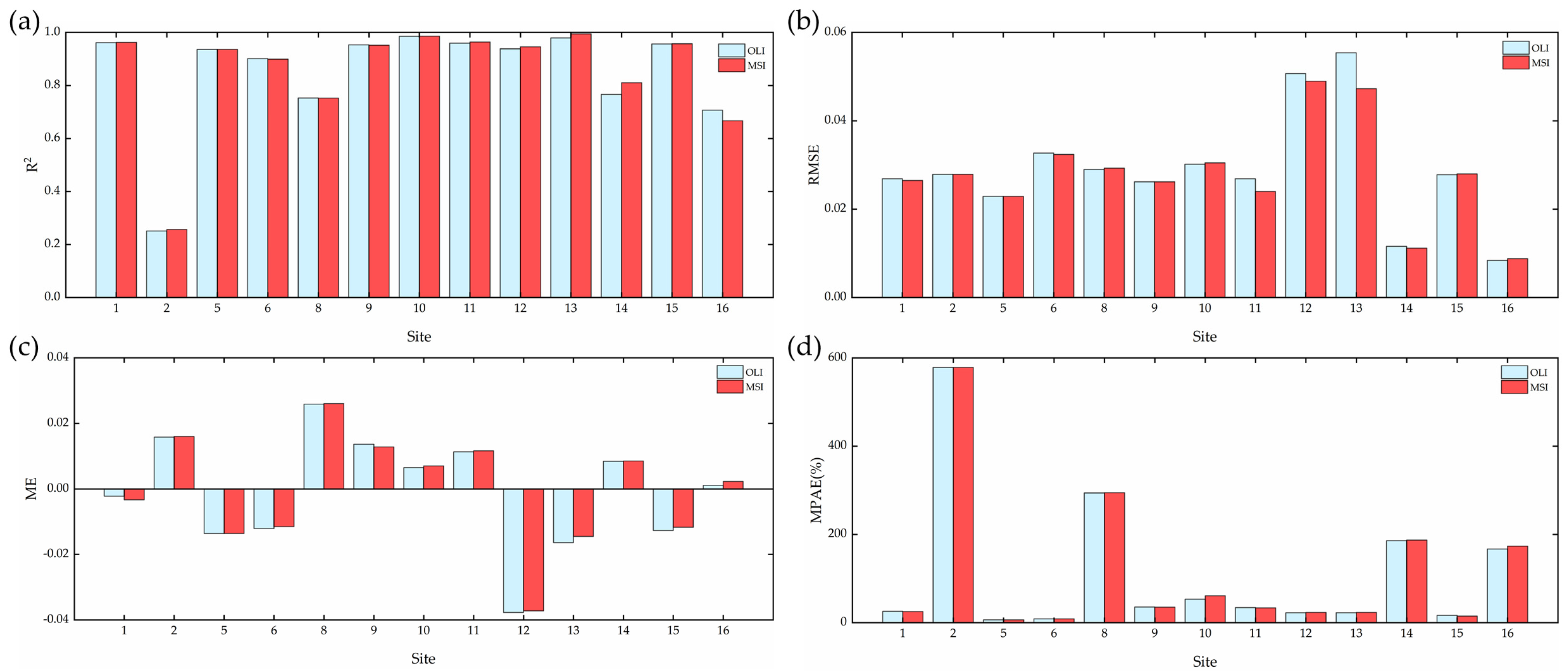
4.1. Validation and Evaluation Results of Two Sensors

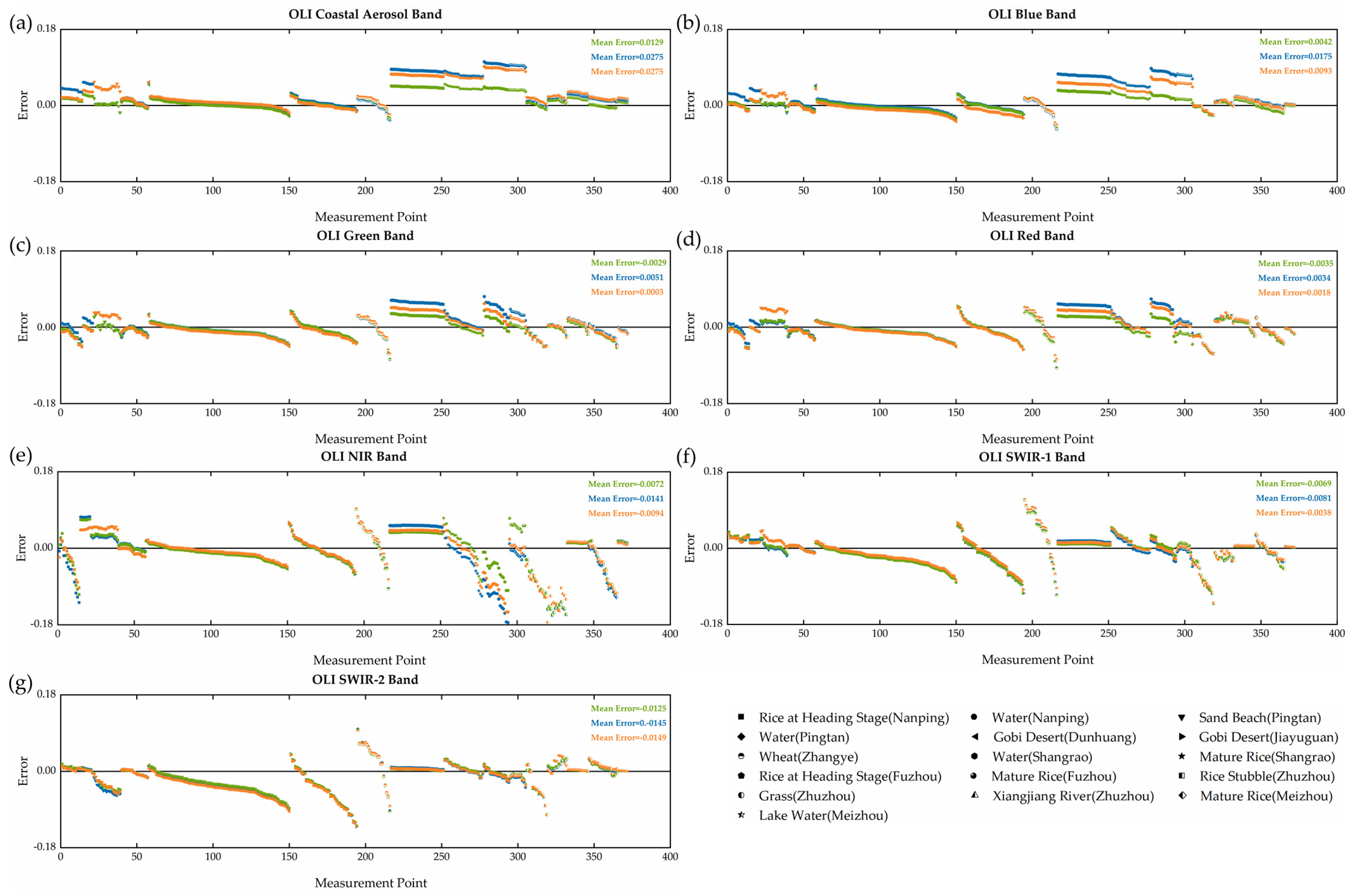
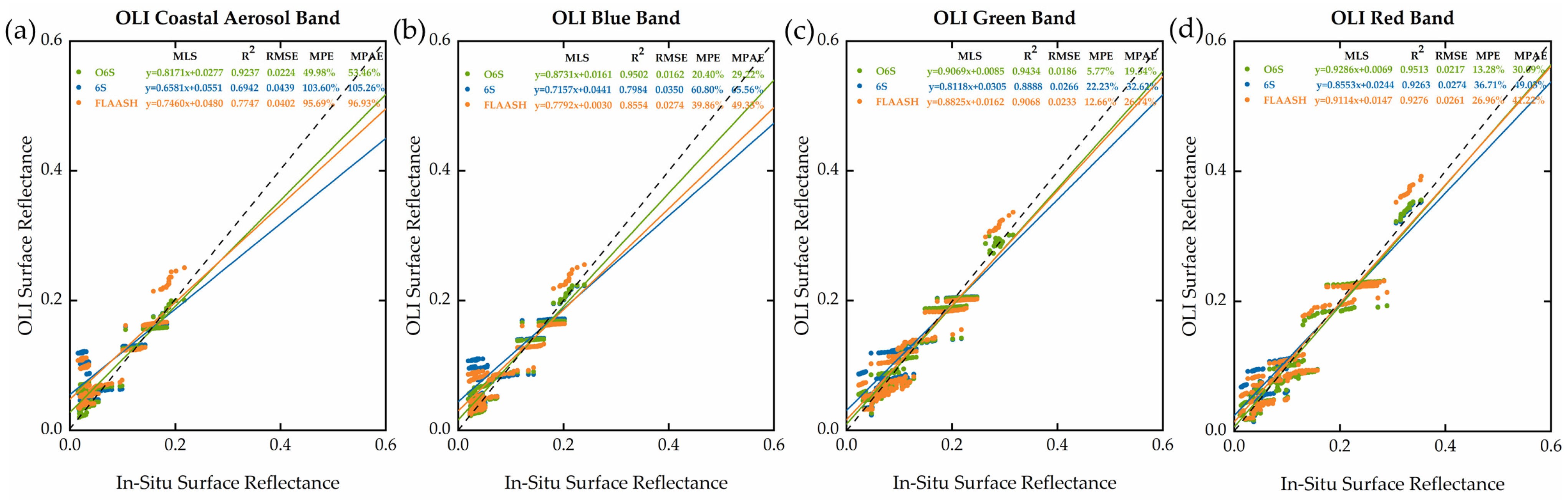
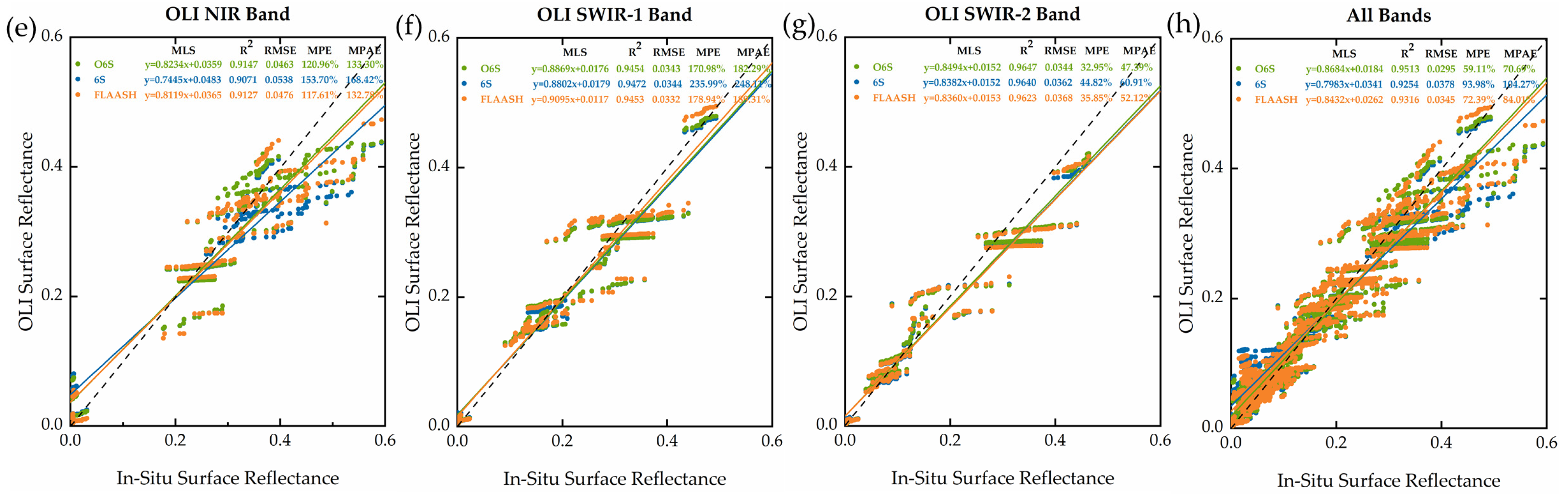
4.1.1. Landsat-8 OLI SR Validation and Evaluation Results

Figure 5 shows scatter plots of the OLI SR product versus the measured SR values at each site. The MLS clearly shows the linear relationship between the OLI SR product and measured values. The difference between the Landsat-8 OLI SR product and the measured values was calculated by linear regression. The values of R², RMSE, MPE, and MPAE of each band were also computed. According to the spectral response function of each sensor, the hyperspectral in situ measurements were weighted before comparing the accuracy.

When considering the synchronous measured data, the MLS slopes ranged from approximately 0.6581 to 0.9286, across all sites and all methods. The measurements showed relatively high agreement with OLI surface reflectance product across all bands (except Coastal Aerosol band), as indicated by R² values were higher than 0.85 (the estimated R² value of Red band, SWIR-1 band, and SWIR-2 band reached about 0.95). Retrieval at the Coastal Aerosol band was the most difficult as indicated by the slopes of 0.8171, 0.6581and 0.7460 (according to the order of methods). However, the RMSE value of the NIR band was obviously higher than that of other bands by three methods. The minimum RMSE value was 0.0463 even after optimization. In terms of specific methods, compared with the original 6S model and FLAASH model, the optimized 6S with auxiliary data had a higher accuracy according to various indicators, especially in the Coastal Aerosol and Blue bands. For the Coastal Aerosol band, the MLS slope was raised to 0.8171, R² value was raised to 0.9237 and RMSE value was reduced to 0.0224, the MPAE value was reduced by 49.21% and 55.43%, respectively. For the Blue band, the MLS slope was raised to 0.8731, the R² value was raised to 0.9502, and the RMSE value was reduced to 0.0162, the MPAE value was reduced by 55.43% and 40.77%. The magnitude agreement between surface reflectance and in situ measurements is better than 40.76%, 38.63%, 20.85%, 26.53%, and 22.20% of the original 6S model, for Green, Red, NIR, SWIR-1, and SWIR-2 bands, respectively.

Figure 6 shows the residual plots of the OLI SR product and the corresponding measured surface reflectance values. From the residual plot of each band, the ME values of the Blue, Green, and Red bands were the smallest, the larger ME value was observed in the NIR band. From the residual plot of each target, the ME values of Gobi in Dunhuang and Jiayuguan were relatively small. The ME values of the mature rice in Fuzhou, rice stubble, and grass in Zhuzhou were relatively large, and the reflectance values are obviously larger than the measurements. The OLI surface reflectance of rice and grass in the NIR band was significantly lower than in situ surface reflectance, and that of water was significantly higher than the in situ surface reflectance. According to the errors of different methods, the optimized 6S model had the minimum mean error as a whole.

The validation results of the OLI SR product were different across all sites. Therefore, we conducted further analysis to validate the accuracy of the product. Here we only analyzed optimized 6S results that had been verified with higher accuracy.

Table 3. RMSE and MPAE values for individual ground truth sites.

Site		Statistics	Coastal	Blue	Green	Red	NIR	SWIR-1	SWIR-2
1	Rice at Heading Stage (Nanping)	RMSE	0.0412	0.0058	0.0230	0.0249	0.0528	0.0279	0.0097
		MPAE (%)	67.19	16.72	20.36	24.39	9.19	24.26	18.02
2	Water (Nanping)	RMSE	0.0234	0.0098	0.0047	0.0069	0.0670	0.0152	0.0042
		MPAE (%)	67.47	23.53	6.12	11.06	1385.71	4543.20	130.68
3	Sand Beach (Pingtan)	RMSE	0.0065	0.0064	0.0112	0.0135	0.0304	0.0103	0.0358
		MPAE (%)	2.54	2.48	2.95	3.92	8.17	1.62	7.72
4	Water (Pingtan)	RMSE	0.0082	0.0064	0.0104	0.0144	0.0067	0.0064	0.0070
		MPAE (%)	29.75	15.76	13.91	24.85	66.51	221.51	69.84
5	Gobi Desert (Dunhuang)	RMSE	0.0098	0.0119	0.0154	0.0164	0.0196	0.0327	0.0384
		MPAE (%)	4.45	5.23	5.61	5.40	6.32	8.24	9.96
6	Gobi Desert (Jiayuguan)	RMSE	0.0097	0.0114	0.0179	0.0232	0.0271	0.0457	0.0600
		MPAE (%)	6.24	6.64	7.47	7.93	8.77	10.49	13.31
7	Wheat (Zhangye)	RMSE	0.0151	0.0196	0.0278	0.0373	0.0474	0.0691	0.0544
		MPAE (%)	24.09	18.24	16.45	16.63	13.67	25.75	32.27
8	Water (Shangrao)	RMSE	0.0438	0.0326	0.0278	0.0246	0.0378	0.0100	0.0050
		MPAE (%)	174.27	126.03	95.37	143.32	687.09	590.91	241.87
9	Mature Rice (Shangrao)	RMSE	0.0117	0.0049	0.0018	0.0026	0.0104	0.0054	0.0027
		MPAE (%)	142.70	50.37	8.87	12.51	8.87	11.50	13.86
10	Rice at Heading Stage (Fuzhou)	RMSE	0.0403	0.0218	0.0194	0.0218	0.0557	0.0156	0.0097
		MPAE (%)	188.46	78.28	26.60	50.86	10.26	8.08	10.62
11	Mature Rice (Fuzhou)	RMSE	0.0364	0.0141	0.0062	0.0195	0.0529	0.0125	0.0135
		MPAE (%)	142.54	37.91	5.36	19.03	15.88	6.33	11.83
12	Rice Stubble (Zhuzhou)	RMSE	0.0056	0.0145	0.0309	0.0424	0.0792	0.0782	0.0508
		MPAE (%)	12.02	18.27	26.73	29.13	29.56	23.99	18.43
13	Grass (Zhuzhou)	RMSE	0.0106	0.0064	0.0083	0.0193	0.1415	0.0222	0.0190
		MPAE (%)	35.67	19.37	6.23	50.26	25.98	7.71	13.01
14	Xiangjiang River (Zhuzhou)	RMSE	0.0162	0.0104	0.0097	0.0128	0.0115	0.0041	0.0023
		MPAE (%)	70.25	36.07	21.52	72.41	601.06	308.24	156.44
15	Mature Rice (Meizhou)	RMSE	0.0036	0.108	0.0227	0.0215	0.0599	0.0233	0.0137
		MPAE (%)	11.76	24.22	18.90	18.03	13.08	11.07	18.71
16	Lake Water (Meizhou)	RMSE	0.0070	0.0009	0.0105	0.0098	0.0150	0.0034	0.0013
		MPAE (%)	36.28	3.22	22.26	29.40	442.23	530.07	104.85

shows the RMSE and MPAE values between obtained OLI SR product and in situ measurements of each site.

Combined with Figure 6, analysis was carried out from each band. In the Coastal and Blue bands, the SR product showed a certain difference when compared to in situ measurements. Reflectance at this level is related to rice at the heading stage, mature rice in Fuzhou, and water in Shangrao with RMSE values around 0.04. Sand beach in Pingtan, Gobi in Dunhuang, and Jiayuguan showed good agreement with measurements: the RMSE values were lower than 0.01 and the MPAE values did not exceed 10%. In the Green and Red bands, the accuracy of vegetation has been improved especially for rice at the heading stage, mature rice in Fuzhou. RMSE values reduced by 50% or more and the MPAE values dropped to about 20%. Other sites also had high accuracy in the two bands. In the NIR band, RMSE values were larger than those of the first four bands, reflectance at that level is associated with the vegetation dominant sites. Vegetation in the NIR band has a high reflectance platform, but is usually lower than the measurements, the RMSE values exceeded 0.05. Although vegetation had a large RMSE value in the NIR band, the MPAE value was relatively low, the MPAE value was basically below 20%. On the contrary, the RMSE value of water was relatively low, but the MPAE value was high. OLI SR product was more accurate in bare land, with a maximum MPAE value of 13.31%. In the SWIR-1 and SWIR-2 bands, the reflectance of vegetation decreased, which was consistent with the measurements. The reflectance of rice stubble in Zhuzhou was different from other vegetation in the two bands, and the rising reflectance value was close to that of the bare land. The RMSE values of bare land in these two bands increased with the increase of reflectance values, but the MPAE remained around 10%.

Generally, across all bands, the rice stubble in Zhuzhou and water in Shangrao sites showed the most spread and variation between OLI and in situ measurements. Both errors were concentrated in the long-wavelength bands. RMSE values of rice stubble in Zhuzhou ranged from 0.05 to 0.08. The MPAE of water in Shangrao increased sharply after the NIR band. For bare land, retrievals at the sand beach site in Pingtan and the Gobi site in Dunhuang and Jiayuguan provided a much closer match to the in situ measurements across all bands.

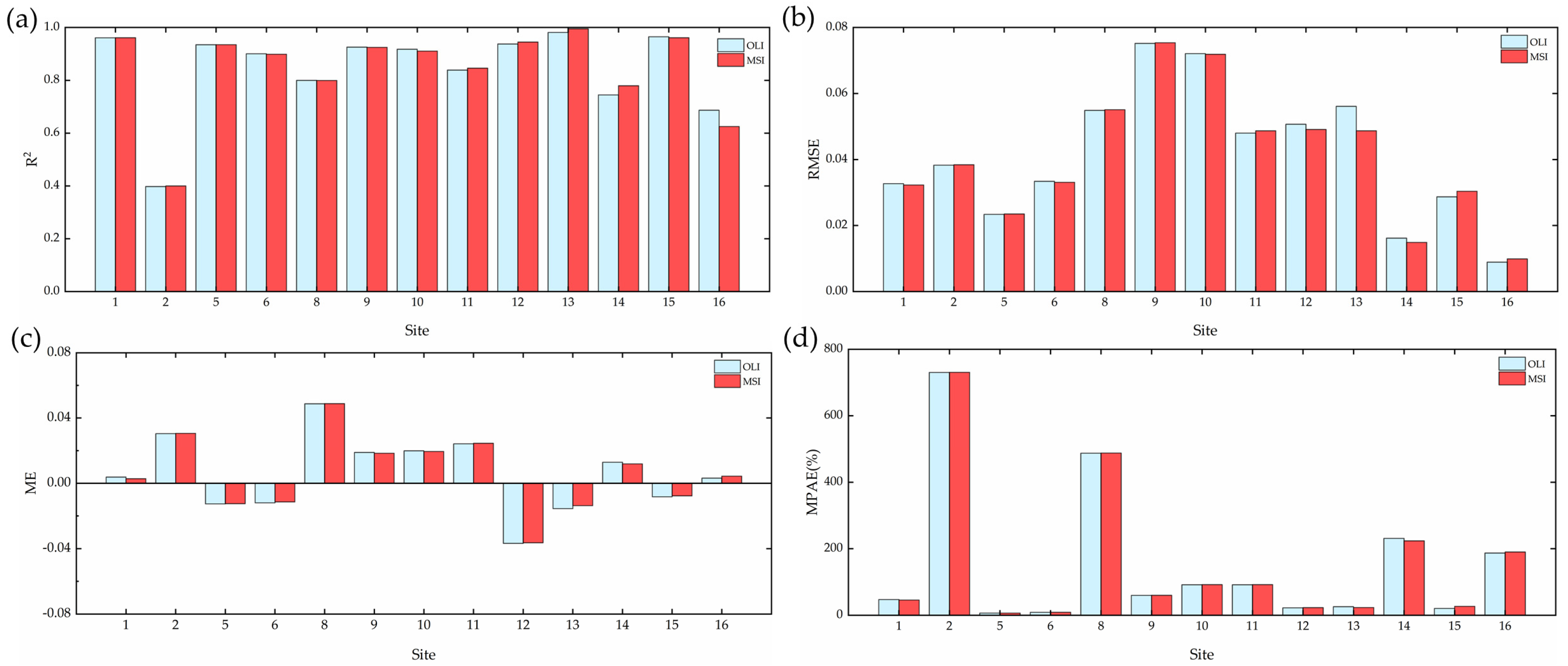
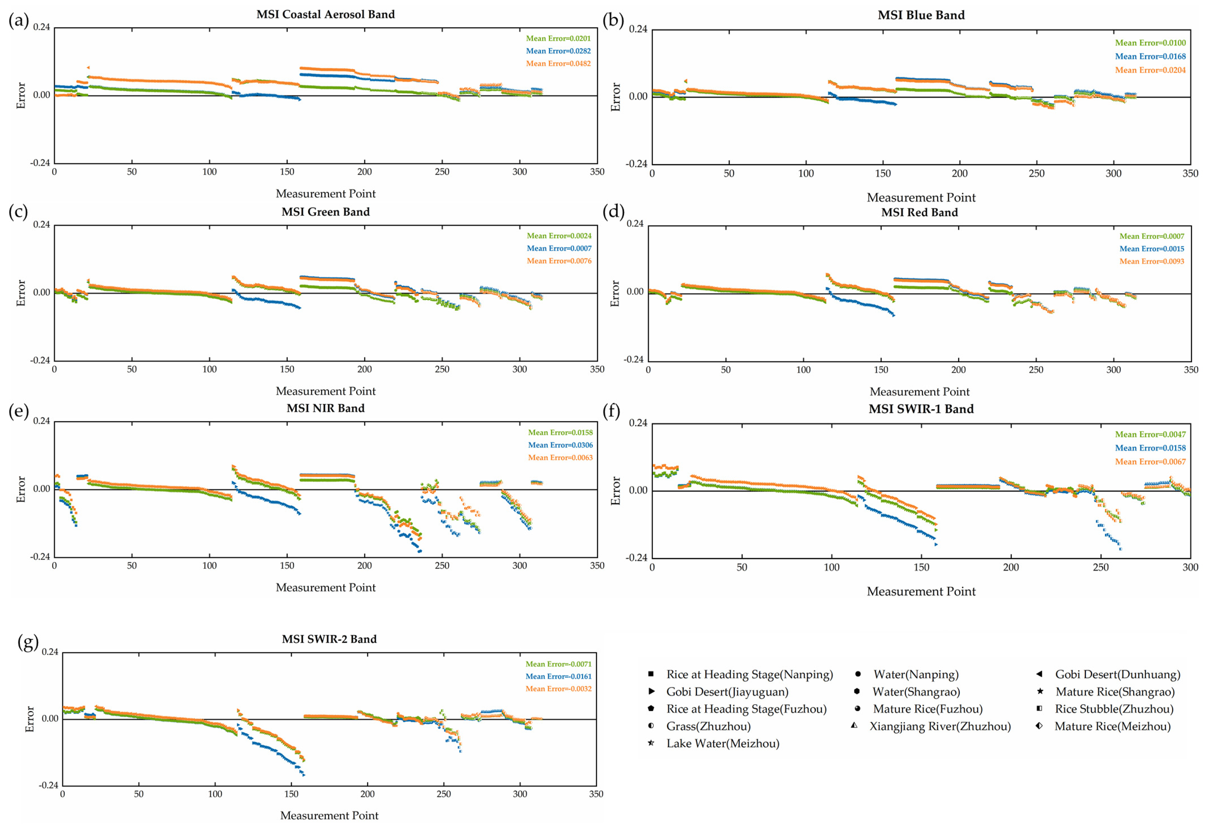
4.1.2. Sentinel-2 MSI SR Validation and Evaluation Results

Figure 7 shows scatter plots of the Sentinel-2 MSI surface reflectance product and measured surface reflectance values. The slopes of MLS ranged from 0.6393 to 1.0586, across all sites and all methods. Since there was no Sentinel-2 MSI overpass image at Pingtan test site in Fujian, the evaluation data did not contain the Pingtan test site. For all sites, the estimated RMSE results were very similar to the corresponding OLI results. The accuracy of the NIR band reflectance was relatively low, while the RMSE values of the other bands were relatively small. Similarly, the optimized 6S significantly improved the accuracy of each band. The optimization effect of the Coastal Aerosol band was the most obvious. In the Coastal Aerosol band, the RMSE values of the 6S and FLAASH models were 0.0370 and 0.0543, and the estimated R² values were 0.8493 and 0.8591, respectively. After optimization, the RMSE value was reduced to 0.0252 and the R² value was raised to 0.9501. The RMSE value decreased by 31.89% and 53.59%, and R² increased by 11.87% and 10.59%. For MSI sensors, optimized 6S still had the highest accuracy compared to the other two methods.

Figure 8 shows the residual plots of the Sentinel-2 MSI surface reflectance data and the corresponding measured surface reflectance values. It can be seen that the mean errors of all spectral bands are positive (except for the SWIR-2 band), especially Coastal Aerosol and Blue bands, that is, the MSI sensor tends to overestimate the true reflectance of the ground. Similar to the OLI sensor results, the mean errors of the Green and Red bands were the smallest; the mean errors of the Coastal and NIR bands were relatively larger. From the residual plot of each site, the accuracy of Gobi in Dunhuang was the highest and the mean error was the minimum. The errors of rice in Fuzhou, rice stubble, and grass in Zhuzhou were relatively large, and most of them were lower than the measurements. From the different methods of each band, the results of the optimized 6S model also had the highest accuracy as a whole.

Table 4. RMSE and MPAE values for individual ground truth sites.

Site		Statistics	Coastal	Blue	Green	Red	NIR	SWIR-1	SWIR-2
1	Rice at Heading Stage (Nanping)	RMSE	0.0177	0.0075	0.0151	0.0152	0.0593	0.0615	0.0299
		MPAE (%)	83.30	20.68	11.55	15.84	11.86	52.28	53.75
2	Water (Nanping)	RMSE	0.0043	0.0050	0.0133	0.0148	0.0408	0.0175	0.0069
		MPAE (%)	11.81	9.64	18.26	31.09	478.61	5258.24	201.72
5	Gobi Desert (Dunhuang)	RMSE	0.0196	0.0130	0.0119	0.0132	0.0132	0.0179	0.0205
		MPAE (%)	11.69	6.21	4.15	4.53	4.02	4.33	5.06
6	Gobi Desert (Jiayuguan)	RMSE	0.0486	0.0341	0.0241	0.0255	0.0281	0.0659	0.0741
		MPAE (%)	39.64	23.28	11.29	9.35	9.48	15.53	16.83
8	Water (Shangrao)	RMSE	0.0293	0.0260	0.0210	0.0222	0.0333	0.0129	0.0079
		MPAE (%)	116.70	98.81	70.63	137.45	526.82	747.20	371.62
9	Mature Rice (Shangrao)	RMSE	0.0216	0.0094	0.0199	0.0154	0.0486	0.0224	0.0149
		MPAE (%)	74.45	15.62	14.84	14.28	10.73	10.69	14.19
10	Rice at Heading Stage (Fuzhou)	RMSE	0.0125	0.0067	0.0174	0.0145	0.1214	0.0076	0.0063
		MPAE (%)	58.99	19.99	17.23	28.95	26.05	4.49	8.14
11	Mature Rice (Fuzhou)	RMSE	0.0078	0.0040	0.0225	0.0296	0.0160	0.0104	0.0065
		MPAE (%)	30.36	6.69	23.59	33.65	4.16	4.80	4.92
12	Rice Stubble (Zhuzhou)	RMSE	0.0084	0.0211	0.0406	0.0501	0.0863	0.0732	0.0463
		MPAE (%)	13.47	30.35	39.22	37.09	35.90	22.96	18.97
13	Grass (Zhuzhou)	RMSE	0.0082	0.0059	0.0202	0.0071	0.1145	0.0246	0.0058
		MPAE (%)	27.31	7.80	21.91	16.73	20.98	7.68	3.88
14	Xiangjiang River (Zhuzhou)	RMSE	0.0205	0.0136	0.0087	0.0120	0.0209	0.0139	0.0120
		MPAE (%)	88.09	45.24	20.00	79.40	672.13	972.61	694.92
15	Mature Rice (Meizhou)	RMSE	0.0061	0.0072	0.0282	0.0258	0.0727	0.0236	0.0161
		MPAE (%)	23.90	12.78	25.29	22.85	18.02	11.72	14.88
16	Lake Water (Meizhou)	RMSE	0.0079	0.0011	0.0148	0.0101	0.0234	0.0063	0.0025
		MPAE (%)	43.81	6.43	30.47	33.91	1030.98	938.79	206.05

shows the RMSE and MPAE values between obtained MSI SR product and in situ measurements of each site.

4.2. Accuracy Comparison of Two Kinds of Reflectance Products

In order to avoid the possible deviation caused by different methods, the inversion accuracy of Landsat-8 OLI and Sentinel-2 MSI under the same method was compared. The band accuracy of each sensor has been analyzed above (Figure 5, Figure 6, Figure 7 and Figure 8), and the comprehensive accuracy of each site was compared here. There was no corresponding result for sites 3–4 and 7 because there was no corresponding MSI surface product for these sites.

Figure 9 shows the accuracy comparison of two kinds of data by the optimized 6S model. The R², RMSE, MPE, and MPAE values were also computed per site. The accuracy of the OLI and MSI reflectance product was highly consistent.

The R² values showed that the R² values of vegetation were higher than of bare land, but the water was the lowest. The results with two data sources showed that the R² of water in Nanping was very low. R² values of Zhuzhou Xiangjiang river and Meizhou lake water were slightly different. For Zhuzhou Xiangjiang river, the R² value of OLI was 0.7665, and MSI was 0.8107. The R² value for MSI for this site increased by 5.77% compared to OLI. For Meizhou lake water, the R² values of OLI and MSI were 0.7068 and 0.6667, respectively. The R² of MSI decreased by 5.67%. The other sites had high consistency, differing by less than 1.55%.

The RMSE values showed that the larger errors were observed from mature rice in Shangrao, and rice at the heading stage in Fuzhou. The overall RMSE values of the water were low, depending on its low surface reflectance value. Zhuzhou grass showed a larger difference between the two data sources. The RMSE values of OLI and MSI were 0.0543 and 0.0473, with the RMSE value decreasing by 14.62%. The largest difference of other sites between them was only 4.76%.

The ME values of water in Nanping, water in Shangrao, and rice stubble in Zhuzhou, were relatively higher, the errors of rice at heading stage in Nanping, sand beach in Pingtan, and Gobi in Gansu were smaller. Meizhou lake water showed the largest difference between the two data sources, the ME value of MSI was twice that of OLI, even though their ME values were all tiny. The rest of the sites had roughly equal ME values.

The MPAE values were large in all sites of water, because the overall reflectance of water was very low, especially after the NIR band. The MPAE values of bare land were the lowest, the accuracy of the two kinds of reflectance products in bare land was relatively consistent and high. The site with the largest difference in MPAE values between the two data sources was Meizhou lake water.

Figure 10 and Figure 11 show the accuracy comparison of two kinds of data by the 6S model and FLAASH model, respectively. The overall results of the two methods were the same as those of the optimized 6S model; therefore, only optimized 6S comparison results were analyzed. The comparative information of each method is shown in

Table 5. Comparison of reflectance products accuracy of two kinds of data.

Site		Statistics	Optimized 6S	6S	FLAASH
			OLI/MSI	OLI/MSI	OLI/MSI
1	Rice at Heading Stage (Nanping)	R2	0.9612/0.9625	0.9610/0.9613	0.9673/0.9615
		RMSE	0.0269/0.0265	0.0327/0.0323	0.0246/0.0259
		ME	−0.0022/−0.0033	0.0038/0.0028	−0.0039/−0.0022
		MPAE (%)	25.73/25.21	47.15/45.91	26.93/29.41
2	Water (Nanping)	R2	0.02513/0.02567	0.3978/0.4000	0.4826/0.4909
		RMSE	0.0279/0.0279	0.0383/0.0384	0.0224/0.0227/
		ME	0.0158/0.0160	0.0304/0.0306	0.0135/0.0139
		MPAE (%)	578.47/578.69	730.53/730.96	450.14/430.51
5	Gobi (Dunhuang)	R2	0.9358/0.9361	0.9347/0.9350	0.9217/0.9203
		RMSE	0.0229/0.0229	0.0234/0.0235	0.0242/0.0242
		ME	−0.0136/−0.0136	−0.0126/−0.0125	−0.0138/−0.0138
		MPAE (%)	6.46/6.48	6.57/6.60/9.33	7.09/7.14/8.56
6	Gobi (Jiayuguan)	R2	0.9011/0.8992	0.9007/0.8989	0.8940/0.8884
		RMSE	0.0327/0.0324	0.0334/0.0331	0.0330/0.0336
		ME	−0.0121/−0.0115	−0.0120/−0.0114	−0.0140/−0.0122
		MPAE	8.69/8.71	8.90/8.92	9.26/9.33%
8	Mature Rice (Shangrao)	R2	0.9532/0.9518	0.9259/0.9249	0.9360/0.9361
		RMSE	0.0262/0.0262	0.0752/0.0754	0.0345/0.0344
		ME	0.0136/0.0128	0.0189/0.0184	0.0190/0.0183
		MPAE (%)	35.53/35.25	59.86/60.10	52.26/52.21
9	Water (Shangrao)	R2	0.7527/0.7525	0.7999/0.7995	0.7755/0.7747
		RMSE	0.0290/0.0293	0.0549/0.0551	0.0430/0.0427
		ME	0.0259/0.0261	0.0487/0.0488	0.0376/0.0372
		MPAE (%)	294.12/294.72	487.22/487.70	378.69/372.06
10	Rice at Heading Stage (Fuzhou)	R2	0.9853/0.9860	0.9119/0.9107	0.9463/0.9443
		RMSE	0.0302/0.0305	0.0721/0.0719	0.0595/0.0602
		ME	0.0065/0.0070	0.0199/0.0195	0.0157/0.0162
		MPAE (%)	53.31/61.12	140.77/140.61	115.74/129.29
11	Mature Rice (Fuzhou)	R2	0.9596/0.9640	0.8389/0.8462	0.8896/0.8963
		RMSE	0.0269/0.0240	0.0480/0.0487	0.0391/0.0396
		ME	0.0113/0.0116	0.0242/0.0245	0.0202/0.0205
		MPAE (%)	34.13/33.46	91.57/92.12	74.01/75.13
12	Rice Stubble (Zhuzhou)	R2	0.9382/0.9458	0.9376/0.9449	0.9290/0.9310
		RMSE	0.0507/0.0490	0.0507/0.0491	0.0520/0.0487
		ME	−0.0377/−0.0372	−0.0368/−0.0364	−0.0367/−0.0378
		MPAE (%)	22.59/23.26	22.32/23.04	25.73/25.82
13	Grass (Zhuzhou)	R2	0.9793/0.9945	0.9815/0.9951	0.9780/0.9943
		RMSE	0.0554/0.0473	0.0561/0.0487	0.0509/0.0367
		ME	−0.0164/−0.0145	−0.0155/−0.0137	−0.0105/−0.0110
		MPAE (%)	22.60/23.23	25.79/23.23	29.39/18.34
14	Xiangjiang River (Zhuzhou)	R2	0.7665/0.8107	0.7445/0.7797	0.6766/0.7750
		RMSE	0.0116/0.0112	0.0162/0.0149	0.0190/0.0092
		ME	0.0084/0.00853	0.0129/0.0119	0.0148/0.0050
		MPAE (%)	185.74/187.11	231.21/223.72	248.95/132.32
15	Mature Rice (Meizhou)	R2	0.9566/0.9574	0.9649/0.9612	0.9604/0.9576
		RMSE	0.0278/0.0280	0.0287/0.0304	0.0273/0.0292
		ME	−0.0127/−0.0117	−0.0083/−0.0077	−0.0070/−0.0054
		MPAE (%)	16.54/14.92	20.60/26.96	22.58/30.93
16	Lake Water (Meizhou)	R2	0.7068/0.6667	0.6868/0.6248	0.6305/0.5237
		RMSE	0.0084/0.0088	0.0089/0.0099	0.0094/0.0116
		ME	0.0011/0.0023	0.0032/0.0044	0.0028/0.0050
		MPAE (%)	166.90/173.46	187.11/190.28	167.75/176.88

.

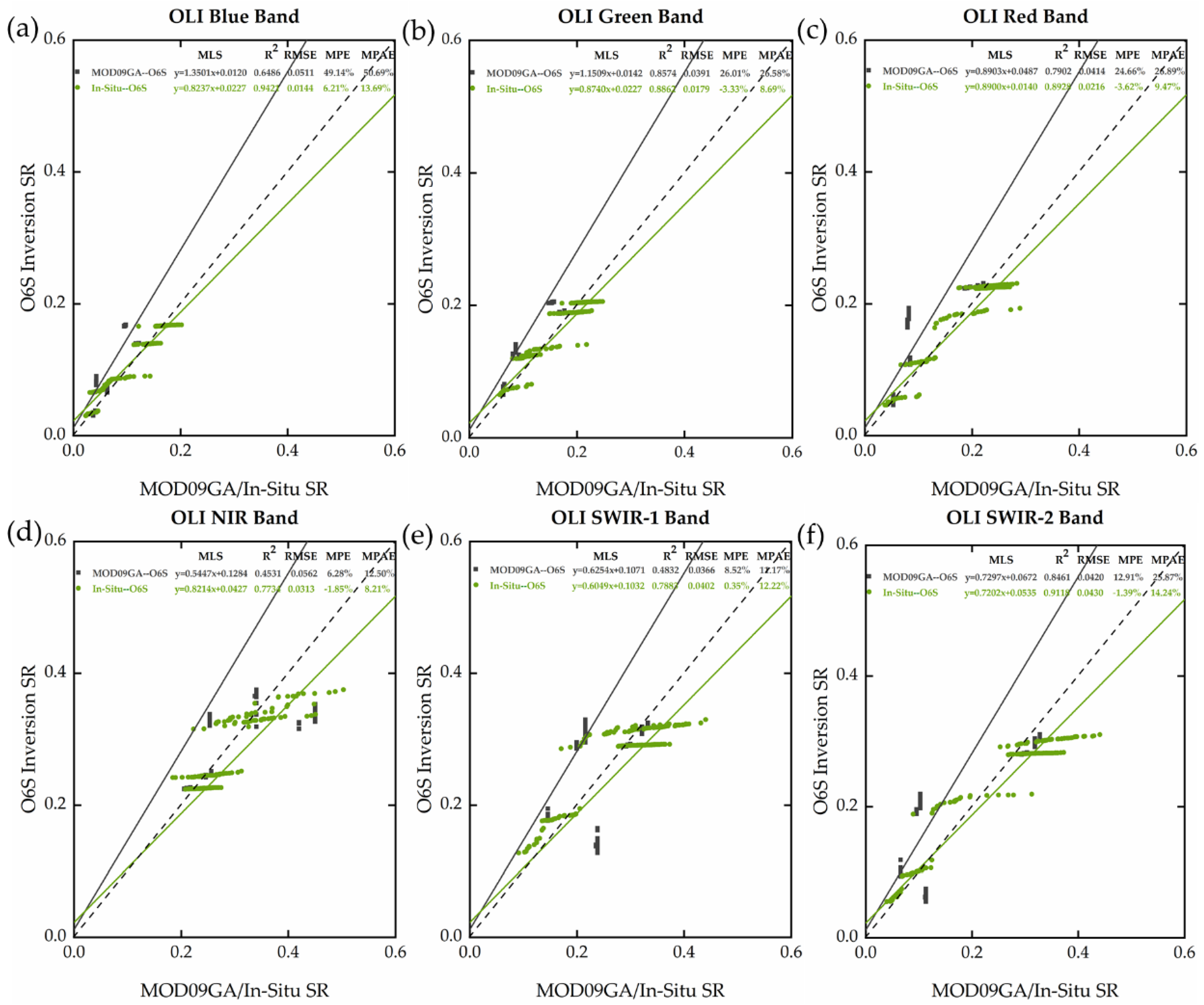
4.3. Accuracy Comparison between Direct and Indirect Validation

We used MOD09GA surface reflectance products to indirectly validate reflectance products obtained from different data sources. The spatial resolution of MOD09GA is 500 m. Since MOD09 has a much lower resolution than OLI, a 3 × 3 MODIS pixel window was used to select pixels from uniform regions. If the difference between the maximum and minimum values of nine pixels is less than the predefined threshold, the central MODIS pixel is considered to be a uniform region [9,21]. Finally, we selected five sites for comparative validation: Nanping rice at heading stage, Dunhuang Gobi, Jiayuguan Gobi, Zhangye wheat, and Shangrao mature rice, in which their area exceeded the MODIS pixel size and was sufficiently homogeneous.

Figure 12 shows the difference between direct and indirect comparisons (taking an optimized 6S model based on OLI sensor as an example). Since MOD09GA does not have a corresponding Coastal Aerosol band, we validated the six OLI bands. In general, the accuracy of MOD09GA validation was much lower than the measured data. At the shorter wavelengths, the reflectance values of MOG09GA were much lower than the inversion values, and the slopes of MLS were greater than 1. At the longer wavelengths, the accuracy of MOD09GA validation of Gobi features was high, and vegetation features were not stable.

The MSI sensor did not include the Zhangye wheat site. The validation results were similar to OLI. The complete comparison results are shown in

Table 6. Comparison results for two kinds of reflectance products between direct and indirect validation.

Sensor	Method	Band	Slope	R2	RMSE	MPE (%)	MPAE (%)
			MO09GA SR/In Situ SR—Reflectance Inversion Values
OLI	O6S	Blue	1.3501/0.8237	0.6468/0.9421	0.0511/0.0144	49.14/6.21	50.69/13.69
		Green	1.1509/0.8740	0.8574/0.8862	0.0391/0.0179	26.01/−3.33	26.58/8.69
		Red	0.8903/0.8928	0.7902/0.8928	0.0414/0.0216	24.66/−3.62	26.89/9.47
		NIR	0.5447/0.8214	0.4531/0.7734	0.0562/0.0313	6.28/−1.85	12.50/8.21
		SWIR-1	0.6254/0.6049	0.4832/0.7883	0.0366/0.0402	8.52/0.35	11.17/12.22
		SWIR-2	0.7297/0.7202	0.8461/0.9118	0.0420/0.0430	12.91/−1.39	25.87/14.24
	6S	Blue	1.1937/0.6959	0.6601/0.8754	0.0545/0.0223	59.66/6.21	59.66/13.69
		Green	1.0599/0.7986	0.8674/0.8824	0.0406/0.0178	29.32/−0.53	29.32/8.67
		Red	0.8347/0.8926	0.7987/0.8926	0.0422/0.0214	27.71/−0.94	28.06/9.11
		NIR	0.5311/0.6953	0.5907/0.7601	0.0476/0.0338	4.35/−3.26	10.66/8.23
		SWIR-1	0.6658/0.6303	0.5025/0.7851	0.0354/0.0399	7.61/−0.53	10.39/11.86
		SWIR-2	0.7257/0.7184	0.8366/0.9070	0.0429/0.0446	11.45/−2.73	25.92/14.32
	FLAASH	Blue	1.1768/0.7343	0.5907/0.8975	0.0479/0.0196	47.35/6.77	50.45/19.37
		Green	1.0643/0.8203	0.8245/0.8777	0.0378/0.0193	25.47/−3.81	26.76/9.93
		Red	0.8250/0.8522	0.7354/0.8871	0.0439/0.0220	26.41/−2.77	29.20/10.12
		NIR	0.5552/0.7938	0.5234/0.8032	0.0522/0.0287	6.97/−1.05	12.54/7.32
		SWIR-1	0.6639/0.6468	0.4749/0.7856	0.0386/0.0383	10.08/1.42	10.60/11.35
		SWIR-2	0.7111/0.7085	0.8258/0.9071	0.0443/0.0463	10.84/−3.56	27.04/14.67
MSI	O6S	Blue	2.0817/0.9951	0.7918/0.9310	0.0707/0.0199	60.74/11.93	62.24/12.98
		Green	1.5039/1.0477	0.9482/0.8945	0.0474/0.0172	28.07/0.43	28.09/8.08
		Red	1.2840/1.0231	0.9887/0.9414	0.0389/0.0175	18.47/2.14	19.54/8.06
		NIR	0.9767/0.5701	0.9079/0.8213	0.0295/0.0302	11.76/−0.87	11.76/6.98
		SWIR-1	0.7447/0.5996	0.6790/0.7802	0.0292/0.0403	6.40/2.35	12.03/11.84
		SWIR-2	0.8822/0.7654	0.9271/0.8812	0.0260/0.0411	6.27/1.53	15.49/13.18
	6S	Blue	1.2760/0.8209	0.4275/0.9102	0.0663/0.0188	61.24/15.34	61.24/19.38
		Green	1.0929/0.9075	0.6495/0.8705	0.0440/0.0181	24.96/−2.60	26.00/8.02
		Red	1.0403/0.8761	0.8340/0.8869	0.0358/0.0227	15.85/−0.24	18.69/9.72
		NIR	0.7496/0.5351	0.5655/0.7654	0.0275/0.0394	5.35/−6.92	11.60/9.09
		SWIR-1	0.6131/0.5113	0.3896/0.4802	0.0479/0.0596	1.34/−2.17	15.51/14.91
		SWIR-2	0.8020/0.6900	0.7779/0.7272	0.0463/0.0618	1.30/−3.09	18.61/16.19
	FLAASH	Blue	1.7863/0.8680	0.7775/0.9445	0.0748/0.0253	72.67/24.15	72.67/24.42
		Green	1.4002/0.9890	0.9409/0.9127	0.0547/0.0181	35.81/6.54	35.81/8.79
		Red	1.2407/0.9920	0.9858/0.9450	0.0453/0.0200	24.68/7.64	24.98/9.92
		NIR	1.0871/0.6163	0.9395/0.8016	0.0409/0.0292	16.83/3.66	16.83/8.11
		SWIR-1	0.8751/0.6553	0.7562/0.7517	0.0356/0.0413	11.44/8.42	13.96/14.41
		SWIR-2	0.9175/0.7880	0.9325/0.8687	0.0256/0.0403	7.53/4.06	14.58/14.71

.

5. Discussion

The best method for validating and evaluating the accuracy of surface reflectance products is using synchronous measurements [44]. This work mainly used three methods to obtain OLI and MSI surface reflectance products: (i) optimized 6S model with auxiliary data, (ii) original 6S model, and (iii) FLAASH model. Discuss this study from the following four aspects.

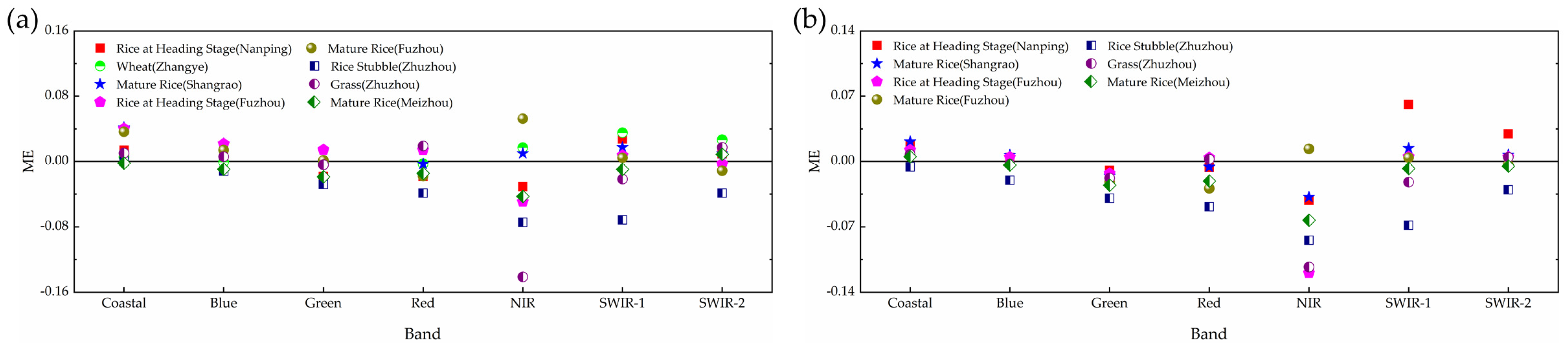
5.1. Accuracy Evaluation of Each Band

The accuracies of OLI and MSI SR products obtained by three methods were compared with the synchronous in situ measurements (Figure 5, Figure 6, Figure 7 and Figure 8). The analysis results show that the optimized 6S model with auxiliary data has the highest accuracy.

For the two kinds of sensors, the accuracy of Coastal Aerosol and Blue bands was the lowest, while the Green and Red bands showed the smallest validation deviations. Aerosols, water vapor, carbon dioxide, and ozone are the main components responsible for most atmospheric perturbations. The degree of atmosphere influence on each band was different: aerosols mainly affect the shorter wavelength bands (Coastal and Blue bands) and water vapor absorption mainly affects the longer wavelength bands (SWIR-1 and SWIR-2 bands) [19].

In the Coastal Aerosol and Blue band, the difference between SR product and measured data was the greatest [18], due to the more difficult inversion of surface reflectance for these bands—the presence of aerosols causes the Rayleigh scattering effect, especially for vegetation targets. This reflects the difficulty of performing atmospheric corrections reliably at shorter wavelengths. The input aerosol parameters in the 6S original model were insufficient (the default AOD is 0.14497), thus the retrieved SR was overestimated, which is also the reason for the large difference at shorter wavelengths. Therefore, the optimized 6S model adjusted the AOD and improved significantly at shorter wavelengths. It should be pointed out that atmospheric correction can never reach the optimal state and can only restore the true surface reflectance value as far as possible, especially at shorter wavelengths where atmospheric effects are usually greatest [13,17,45]. The effects of aerosols in the visible spectrum are difficult to correct for two main reasons. Firstly, due to the properties of aerosols [18,46], aerosol concentrations can change rapidly and significantly over time and space. Secondly, aerosols have complex scattering and absorption characteristics; these properties vary with the size, shape, density, and spectrum of aerosols [8]. Considering the accuracy of the derived surface reflectance, it is particularly important to parameterize the characteristics of aerosol models over space and time domains [47].

In the Green and Red bands, all methods had high accuracy, and the accuracy of the optimized 6S model was still the highest. The maximum value of RMSE was 0.0276. The MPE values of all methods were within 40%. The results showed that the influence of the atmosphere on these two bands was obviously lower than other bands [19].

In the NIR band, the RMSE values increased sharply, and the minimum was 0.0463 even after optimization. This is because the NIR band is a special band for both vegetation and water. There are more vegetation and water sites in this study, thus the error is obvious. Vegetation reaches a high reflectance platform in the NIR band, but the surface reflectance of water is close to 0 in this band. It is difficult for achieving such an ideal result.

In the SWIR-1 and SWIR-2 bands, the R² of all methods was almost higher than other bands. However, RMSE and MPAE values were relatively larger, which may be mainly due to the higher reflectance values of bare land and lower reflectance values of water in these two bands. The improvement of accuracy for the two bands was not obvious by the optimized 6S model compared with other bands. At longer wavelengths, however, water vapor is harder to quantify mainly because of its temporal and spatial variability.

As discussed above, the optimized 6S model provided the best performance surpassing all the other models. Thus, the 6S model needs to be corrected with necessary auxiliary data [48,49,50].

5.2. Accuracy Evaluation of Different Cover Types

For different land cover types, the accuracy of bare land is the highest, vegetation is the second and water is the lowest. Basically the same results are obtained by the three methods. Here we only discuss the results of the optimized 6S model. However, even the same type can vary slightly from place to place. Combined with Table 3 and Table 4 and Figure 9, we had the following discussion in more detail.

Figure 13 shows the mean reflectance difference between OLI/MSI SR products and in situ measurements for all vegetation sites. It indicates that the Zhuzhou rice stubble suffers from the largest errors in estimated surface reflectance (ME of up to −0.0377 and −0.0372, respectively) while the Meizhou mature rice site feature the smallest errors with MPAE of 16.54% (OLI) and 14.92% (MSI), respectively. This may be because the rice stubble is less homogeneous than other mature rice sites. Rice stubble also has no typical spectral characteristics of vegetation in these bands. It is obvious that Zhuzhou grass had small errors in all bands except the NIR band. This is because the measured reflectance of grass in this band was very high, exceeding 0.50, while the inversion reflectance did not achieve such an ideal effect, and the reflectance values were basically about 0.43. As a matter of fact, the results of almost all vegetation sites in the NIR band were lower than the measured data. This may be due to the strong reflection and transmission characteristics of vegetation in this band. At the same time, the reflectance of the near-ground observation was easily affected by the repeated reflection of the transmitted light through the lower blade, so the results of the near-ground observation were higher than those of the satellite sensor. The mean errors of vegetation sites in the last three bands were significantly higher than those in the first four bands, which depends on the reflectance values of each band, the MPAE values were just the opposite.

Figure 14 shows the mean reflectance difference between OLI/MSI SR products and in situ measurements for all water sites. In the shorter wavelength bands, the reflectance of deep water is higher than that of shallow water; in the longer wavelength bands, there is little difference between them. SR products consistently overestimate the measured reflectance, as evidenced by the mean errors of most sites above 0 for all bands. There are probably two main reasons. On the one hand, the reflectance of water is very low, especially after the NIR band; on the other hand, water is fluid and not as stable as other land objects. The ME and RMSE value of all water sites were relatively low, but the MPAE values were high. The reason is the water reflectance in the NIR and SWIR bands were essentially 0 [19], even for extremely turbid waters [51], a small absolute change in the number can result in a large percentage change. This makes both measurement and inversion difficult.

Figure 15 shows the mean reflectance difference between OLI/MSI SR products and in situ measurements for all bare land sites. It shows that bare land sites provided the best validation accuracy with ME values below 0.08 [52]. This could be explained by the fact that bare land sites mostly experience clear skies. Another rationale could be the spectral reflectance of barren ground, which tends to be flatter than that of vegetation [52]. Beach and desert reflectance curves are different. This may be due to the fact that the concrete composition of different bare-ground materials is not quite the same. At the Pingtan sand beach site, the measured sand was moist because it was constantly buffeted by the sea currents. The Gobi is composed of gravel, fine sand, and a small amount of clay. The MPAE values of the two data were 6.46% and 6.48% at the Dunhuang Gobi site and 8.69% and 8.71% at the Jiayuguan Gobi site, respectively. This also proves that, even the same Gobi, the Dunhuang Correction Field has higher accuracy, which depends on the advantages of its unique geographical location and atmospheric conditions.

5.3. Accuracy Comparison of Different Data

The accuracy of the two kinds of reflectance products was compared using the same method (Figure 9, Figure 10 and Figure 11 and Table 3 and Table 4). The accuracy of the OLI SR product and MSI SR product was highly consistent at each site even though they did not cross on the same day. This confirmed the previous hypothesis that the surface did not change much between the two observations. The differences in spatial resolution between the OLI and MSI have a negligible effect on the results showing that the almost sites variability is stable at various scales below the full measurement area [53]. The best results here are found over the Dunhuang Gobi region, despite the mismatch in measurement and MSI overpass time. It should be pointed out that the accuracy comparison results of the OLI image on 22 October and MSI image on 19 October are different for different ground objects. The difference between the two kinds of the data source of Meizhou mature rice was much smaller than that of Meizhou lake water. Although the overpass time of Landsat-8 and Sentinel-2 were three days apart, the bigger reason should be that the water has the characteristics of fluidity and instability.

Comparing different validation methods (Figure 12 and Table 6) indicated that due to the difference of sensors and the limitation of resolution between MOD09GA and OLI/MSI, the validation accuracy of MOD09GA in shorter wavelengths is lower than the measured data. MOD09GA data were unstable for vegetation. In the SWIR-1 and SWIR-2 bands, the reflectance of MOD09GA of Nanping rice was significantly higher than the inversion values, while the reflectance of MOD09GA of Shangrao rice was significantly lower than the measured values. The inversion values were normally distributed around the measured data. MOD09GA is suitable for validating large and uniform features such as Dunhuang Gobi, but it may be challenging if we want to validate specific features due to its much lower spatial resolution. Again, it’s more important to emphasize that MOD09GA data has one of its biggest drawbacks, which is that it cannot be used to validate water. For MODGA09 data, the reflectance of the water does not conform to the normal reflectance characteristics of the water, and its reflectance value is obviously high. This is also the reason why we did not choose water sites in the comparison work. Synchronous measurements ensure the traceability of the data and eliminate these challenges.

5.4. Limitation and Future Perspectives

The optimized 6S model had improved accuracy in all bands for OLI and MSI data, the results show that the improvement effect is significant in shorter wavelength bands, while the improvement effect is not obvious in longer bands, especially for water features with their reflectance close to 0. We need to continuously improve the accuracy of the calculation of the surface reflectance in future studies, then apply the method to the different data and objects as much as possible. In the actual measurement, due to the short overpass time of the satellite, we cannot measure many kinds of ground objects at the same time, but can only measure representative cover types. For vegetation, the spectra of rice and wheat were mainly collected in this study, while other crops were not involved. Although we measured the spectral data of Pingtan sweet potato leaves and Zhangye oats, the measured data showed great fluctuation, because of sparse leaves, the influence of soil, and a large area of lodging oats. We had to eliminate these data so that we didn’t compare the reflectance of many crops. The ground objects in the measurement field should be single and stable, with flat terrain, uniform surface, and good directional characteristics. Despite adopting the optimal measured data after screening, the accuracy of the Dunhuang correction field was still the highest, vegetation and water did not achieve such high precision.

The comparisons are shown in Figure 9, Figure 10 and Figure 11 and Table 5 demonstrate that the agreement between the corresponding sites of Landsat-8 OLI and Sentinel-2 MSI sensors is very good, confirming the potential of combined use of Landsat-8 OLI and Sentinel-2 MSI products. However, we did not consider the agreement between the corresponding bands of sensors. We intend to discuss this issue in-depth in our upcoming work. What are the mechanisms for establishing the most direct and accurate relationship? If we want to carry out linear fitting between the measured data (the hyperspectral in situ measured values are weighted according to the spectral response function of each sensor) and the reflectance products of each band, we need to discuss whether the fitting function is related to specific methods. In order to test this hypothesis, it seems likely that a number of careful experimentation would be required. Of course, we also need to consider that the fitting function may have substantial regional differences, and we also can determine whether the discrepancies in reflectance values are relevant or not for each specific object.

6. Conclusions

In this study, the in situ measurements of surface reflectance synchronized with satellite data were obtained in large areas of China. Compared with indirect verification, it provided effective support for the accurate validation of satellite remote sensing surface reflectance products.

The optimized 6S, original 6S model, and FLAASH model were used to retrieve the surface reflectance of Landsat-8 OLI and Sentinel-2 MSI satellite data, and the accuracy analysis showed that the optimized 6S model had the highest accuracy among the three models. It can improve the accuracy of two kinds of satellite surface reflectance products.

Although the overpass times of the two sensors, OLI and MSI, are not completely synchronized, the accuracy of each site is highly consistent. In other words, the difference between the two sensors is minimal, and the combination of OLI and MSI sensors offers unprecedented possibilities for high-frequency time series analysis, greatly alleviating the problem of data not being available due to cloud coverage.

References

1. Nazeer, M.; Wong, M.S.; Nichol, J.E. A new approach for the estimation of phytoplankton cell counts associated with algal blooms. Sci. Total Environ. 2017, 590–591, 125–138. [Google Scholar] [CrossRef] [PubMed]
2. Nazeer, M.; Ilori, C.O.; Bilal, M.; Nichol, J.E.; Wu, W.; Qiu, Z.; Gayene, B.K. Evaluation of atmospheric correction methods for low to high resolutions satellite remote sensing data. Atmos. Res. 2021, 249, 105308. [Google Scholar] [CrossRef]
3. Vermote, E.F.; Tanré, D.; Deuze, J.L.; Herman, M.; Morcette, J.J. Second simulation of the satellite signal in the solar spectrum, 6S: An overview. IEEE Trans. Geosci. Remote. Sens. 1997, 35, 675–686. [Google Scholar] [CrossRef] [Green Version]
4. Wu, X.; Wen, J.; Xiao, Q.; Yu, Y.; You, D.; Hueni, A. Assessment of NPP VIIRS Albedo Over Heterogeneous Crop Land in Northern China. J. Geophys. Res. Atmos. 2017, 122, 113–138. [Google Scholar] [CrossRef] [Green Version]
5. Yumimoto, K.; Nagao, T.M.; Kikuchi, M.; Sekiyama, T.T.; Murakami, H.; Tanaka, T.Y.; Ogi, A.; Irie, H.; Khatri, P.; Okumura, H.; et al. Aerosol data assimilation using data from Himawari-8, a next-generation geostationary meteorological satellite. Geophys. Res. Lett. 2016, 43, 5886–5894. [Google Scholar] [CrossRef]
6. Zhang, H.; Kondragunta, S.; Laszlo, I.; Liu, H.; Remer, L.A.; Huang, J.; Superczynski, S.; Ciren, P. An enhanced VIIRS aerosol optical thickness (AOT) retrieval algorithm over land using a global surface reflectance ratio database. J. Geophys. Res. Atmos. 2016, 121, 10717–10738. [Google Scholar] [CrossRef]
7. Giannis, L.; Zina, M.; Nektarios, C. Comparison of physically and image based atmospheric correction methods for Sentinel-2 satellite imagery. In Proceedings of the Fourth International Conference on Remote Sensing and Geoinformation of the Environment (RSCy2016), Paphos, Cyprus, 4–8 April 2016. [Google Scholar]
8. Eric, V.; Chris, J.; Martin, C.; Belen, F. Preliminary analysis of the performance of the Landsat 8/OLI land surface reflectance product. Remote Sens. Environ. 2016, 185, 46–56. [Google Scholar]
9. Wang, Y.; Liu, L.; Hu, Y.; Li, D.; Li, Z. Development and validation of the Landsat-8 surface reflectance products using a MODIS-based per-pixel atmospheric correction method. Int. J. Remote Sens. 2016, 37, 1291–1314. [Google Scholar] [CrossRef]
10. Neil, F.; Clement, A.; Prasad, S.T. Comparing Sentinel-2A and Landsat 7 and 8 Using Surface Reflectance over Australia. Remote Sens. 2017, 9, 659. [Google Scholar]
11. Muhammad, B.; Majid, N.; Janet, E.N.; Max, P.B.; Qiu, Z.; Evelyn, J.; James, R.C.; Luqman, A.; Huang, X.; Simone, L. A Simplified and Robust Surface Reflectance Estimation Method (SREM) for Use over Diverse Land Surfaces Using Multi-Sensor Data. Remote Sens. 2019, 11, 1134. [Google Scholar]
12. Lee, K.S.; Lee, C.S.; Seo, M.; Choi, S.; Seong, N.H.; Jin, D.; Yeom, J.-M.; Han, K.-S. Improvements of 6S Look-Up-Table Based Surface Reflectance Employing Minimum Curvature Surface Method. Asia-Pac. J. Atmos. Sci. 2020, 56, 235–248. [Google Scholar] [CrossRef] [Green Version]
13. Min, F.; Chengquan, H.; Saurabh, C.; Eric, F.V.; Jeffrey, G.M.; John, R.T. Quality assessment of Landsat surface reflectance products using MODIS data. Comput. Geosci.-UK 2012, 38, 9–22. [Google Scholar]
14. Francesco, V.; Matteo, M.; Clement, A. Comparison of the Landsat Surface Reflectance Climate Data Record (CDR) and manually atmospherically corrected data in a semi-arid European study area. Int. J. Appl. Earth Obs. Geoinf. 2015, 42, 1–10. [Google Scholar]
15. Nazeer, M.; Nichol, J.E.; Yung, Y.K. Evaluation of atmospheric correction models and Landsat surface reflectance product in an urban coastal environment. Int. J. Remote Sens. 2014, 35, 6271–6291. [Google Scholar] [CrossRef]
16. Maiersperger, T.K.; Scaramuzza, P.L.; Leigh, L.; Shrestha, S.; Gallo, K.P.; Jenkerson, C.B.; Dwyer, J.L. Characterizing LEDAPS surface reflectance products by comparisons with AERONET, field spectrometer, and MODIS data. Remote Sens. Environ. 2013, 136, 1–13. [Google Scholar] [CrossRef] [Green Version]
17. Claverie, M.; Vermote, E.F.; Franch, B.; Masek, J.G. Evaluation of the Landsat-5 TM and Landsat-7 ETM + surface reflectance products. Remote Sens. Environ. 2015, 169, 390–403. [Google Scholar] [CrossRef]
18. Moe, B.; Dennis, H.; Larry, L.; Xin, J. Methods for Earth-Observing Satellite Surface Reflectance Validation. Remote Sens. 2019, 11, 1543. [Google Scholar]
19. Cibele, T.P.; Xin, J.; Larry, L. Evaluation Analysis of Landsat Level-1 and Level-2 Data Products Using In Situ Measurements. Remote Sens. 2020, 12, 2597. [Google Scholar]
20. Song, C.; Woodcock, C.E.; Seto, K.C.; Lenney, M.P.; Macomber, S.A. Classification and Change Detection Using Landsat TM Data: When and How to Correct Atmospheric Effects? Remote Sens. Environ. 2001, 75, 230–244. [Google Scholar] [CrossRef]
21. Min, F.; Joseph, O.S.; Huang, C.; Jeffrey, G.M.; Eric, F.V.; Feng, G.; Raghuram, N.; Saurabh, C.; Robert, E.W.; John, R.T. Global surface reflectance products from Landsat: Assessment using coincident MODIS observations. Remote Sens. Environ. 2013, 134, 276–293. [Google Scholar]
22. James, R.I.; John, L.D.; Julia, A.B. The next Landsat satellite: The Landsat Data Continuity Mission. Remote Sens. Environ. 2012, 122, 11–21. [Google Scholar]
23. Drusch, M.; Del Bello, U.; Carlier, S.; Colin, O.; Fernandez, V.; Gascon, F.; Hoersch, B.; Isola, C.; Laberinti, P.; Martimort, P.; et al. Sentinel-2: ESA’s Optical High-Resolution Mission for GMES Operational Services. Remote Sens. Environ. 2012, 120, 25–36. [Google Scholar] [CrossRef]
24. Jian, L.; David, P.R.; Clement, A.; Guoqing, Z. A Global Analysis of Sentinel-2A, Sentinel-2B and Landsat-8 Data Revisit Intervals and Implications for Terrestrial Monitoring. Remote Sens. 2017, 9, 902. [Google Scholar]
25. Homer, C.; Huang, C.; Yang, L.; Wylie, B.; Coan, M. Development of a 2001 National Land-Cover Database for the United States. Photogramm. Eng. Remote Sens. 2004, 70, 829–840. [Google Scholar] [CrossRef] [Green Version]
26. Kaufman, Y.J. Algorithm for Remote Sensing of Tropospheric Aerosol from Modis. In NASA MODIS Algorithm Theoretical Basis Document; Goddard Space Flight Center: Greenbelt, MD, USA, 1998. [Google Scholar]
27. King, M.D.; Tsay, S.C.; Platnick, S.E.; Wang, M.; Liou, K.N. Cloud Retrieval Algorithms for MODIS: Optical Thickness, Effective Particle Radius, and Thermodynamic Phase, MODIS Algorithm Theoretical Basis Document; Cambridge University Press: Greenbelt, MD, USA, 1997. [Google Scholar]
28. Seemann, S.W.; Borbas, E.E.; Li, J.; Menzel, W.P.; Gumley, L.E. MODIS Atmospheric Profile Retrieval Algorithm Theoretical Basis Document; Cooperative Institute for Meteorological Satellite Studies, University of Wisconsin-Madison: Madison, WI, USA, 2006; p. 40. [Google Scholar]
29. Chen, X.; Xing, J.; Liu, L.; Li, Z.; Mei, X.; Fu, Q.; Xie, Y.; Ge, B.; Li, K.; Xu, H. In-Flight Calibration of GF-1/WFV Visible Channels Using Rayleigh Scattering. Remote Sens. 2017, 9, 513. [Google Scholar] [CrossRef] [Green Version]
30. Pandya, M.R.; Pathak, V.N.; Shah, D.B.; Singh, R.P. Retrieval of Surface Reflectance using SACRS2: A Scheme for Atmospheric Correction of ResourceSat-2 AWiFS data. ISPRS-Int. Arch. Photogramm. Remote Sens. Spat. Inf. Sci. 2014, XL-8, 865–868. [Google Scholar] [CrossRef] [Green Version]
31. Sun, Z.; Wei, J.; Zhang, N.; He, Y.; Sun, Y.; Liu, X.; Yu, H.; Sun, L. Retrieving High-Resolution Aerosol Optical Depth from GF-4 PMS Imagery in Eastern China. Remote Sens. 2021, 13, 3752. [Google Scholar] [CrossRef]
32. Prokhorenkova, L.; Gusev, G.; Vorobev, A.; Dorogush, A.V.; Gulin, A. CatBoost: Unbiased boosting with categorical features. In Proceedings of the Advances in Neural Information Processing Systems 31 (NeurIPS 2018), Montréal, QC, Canada, 3–8 December 2018. [Google Scholar]
33. Chair-Krishnapuram, B.G.; Chair-Shah, M.G.; Chair-Smola, A.P.; Chair-Aggarwal, C.P.; Chair-Shen, D.P.; Chair-Rastogi, R.P. Acm Sigkdd International Conference on Knowledge Discovery & Data Mining. In Proceedings of the 22nd ACM SIGKDD International Conference on Knowledge Discovery and Data Mining, San Francisco, CA, USA, 13–17 August 2016. [Google Scholar]
34. Zhang, Y.; Zhao, Z.; Zheng, J. CatBoost: A new approach for estimating daily reference crop evapotranspiration in arid and semi-arid regions of Northern China. J. Hydrol. 2020, 588, 125087. [Google Scholar] [CrossRef]
35. Dorogush, A.V.; Ershov, V.; Gulin, A. CatBoost: Gradient boosting with categorical features support. arXiv 2018, arXiv:1810.11363. [Google Scholar]
36. Hancock, J.; Khoshgoftaar, T.M. CatBoost for Big Data: An Interdisciplinary Review. J. Big Data 2020, 7, 94. [Google Scholar] [CrossRef] [PubMed]
37. Khalid, R.; Javaid, N. A Survey on Hyperparameters Optimization Algorithms of Forecasting Models in Smart Grid. Sustain. Cities Soc. 2020, 61, 102275. [Google Scholar] [CrossRef]
38. Ding, Y.; Chen, Z.; Lu, W.; Wang, X. A CatBoost approach with wavelet decomposition to improve satellite-derived high-resolution PM2.5 estimates in Beijing-Tianjin-Hebei. Atmos. Environ. 2021, 249, 118212. [Google Scholar] [CrossRef]
39. Xue, C.; Chen, S.; Lee, Z.; Hu, L.; Shi, X.; Lin, M.; Liu, J.; Ma, C.; Song, Q.; Zhang, T. Iterative near-infrared atmospheric correction scheme for global coastal waters. ISPRS J. Photogramm. 2021, 179, 92–107. [Google Scholar] [CrossRef]
40. Juan, C.J.; José, A.S.; Cristian, M.; Belen, F. Atmospheric correction of optical imagery from MODIS and Reanalysis atmospheric products. Remote Sens. Environ. 2010, 114, 2195–2210. [Google Scholar]
41. Kotchenova, S.Y.; Vermote, E.F.; Matarrese, R.; Klemm, F.J. Validation of a vector version of the 6S radiative transfer code for atmospheric correction of satellite data. Part I: Path radiance. Appl. Opt. 2006, 45, 6762–6774. [Google Scholar] [CrossRef] [Green Version]
42. Ron, M.; Julia, B.; Raviv, L.; Brian, M.; Esad, M.; Lawrence, O.; Pat, S.; Kelly, V. Landsat-8 Operational Land Imager (OLI) Radiometric Performance On-Orbit. Remote Sens. 2015, 7, 2208–2237. [Google Scholar]
43. Miura, T.; Huete, A.R.; Yoshioka, H. Evaluation of sensor calibration uncertainties on vegetation indices for MODIS. IEEE Trans. Geosci. Remote Sens. 2000, 38, 1399–1409. [Google Scholar] [CrossRef]
44. Dennis, H.; Kurt, T.; Dave, A.; Larry, L.; Jeff, C.; Nathan, L.; Stuart, B.; Nik, A. Recent surface reflectance measurement campaigns with emphasis on best practices, SI traceability and uncertainty estimation. Metrologia 2012, 49, 21–28. [Google Scholar]
45. Junchang, J.; David, P.R.; Eric, V.; Jeffrey, M.; Valeriy, K. Continental-scale validation of MODIS-based and LEDAPS Landsat ETM+ atmospheric correction methods. Remote Sens. Environ. 2012, 122, 175–184. [Google Scholar]
46. Georgia, D.; Eric, V.; Jean-Claude, R.; Ferran, G.; Stefan, A.; David, F.; Olivier, H.; André, H.; Grit, K.; Fuqin, L.; et al. Atmospheric Correction Inter-Comparison Exercise. Remote Sens. 2018, 10, 352. [Google Scholar]
47. Rasmus, H.; Matthew, F.M. Impacts of dust aerosol and adjacency effects on the accuracy of Landsat 8 and RapidEye surface reflectances. Remote Sens. Environ. 2017, 194, 127–145. [Google Scholar]
48. Zhang, H.K.; Roy, D.P.; Yan, L.; Li, Z.; Huang, H.; Vermote, E.; Skakun, S.; Roger, J.-C. Characterization of Sentinel-2A and Landsat-8 top of atmosphere, surface, and nadir BRDF adjusted reflectance and NDVI differences. Remote Sens. Environ. 2018, 215, 482–494. [Google Scholar] [CrossRef]
49. Martin, C.; Junchang, J.; Jeffrey, G.M.; Jennifer, L.D.; Eric, F.V.; Jean-Claude, R.; Sergii, V.S.; Christopher, J. The Harmonized Landsat and Sentinel-2 surface reflectance data set. Remote Sens. Environ. 2018, 219, 145–161. [Google Scholar]
50. David, F.; Marion, S.; Patrick, H. A Global MODIS Water Vapor Database for the Operational Atmospheric Correction of Historic and Recent Landsat Imagery. Remote Sens. 2019, 11, 257. [Google Scholar]
51. Feng, L.; Hou, X.; Li, J.; Zheng, Y. Exploring the potential of Rayleigh-corrected reflectance in coastal and inland water applications: A simple aerosol correction method and its merits. ISPRS J. Photogramm. 2018, 146, 52–64. [Google Scholar] [CrossRef]
52. Tuomiranta, A.; Alet, P.; Ballif, C.; Ghedira, H. Worldwide performance evaluation of ground surface reflectance models. Sol. Energy. 2021, 224, 1063–1078. [Google Scholar] [CrossRef]
53. Niall, O.; Javier, G.; James, R.; Joanne, N.; Agnieszka, B. Fiducial Reference Measurements for validation of Sentinel-2 and Proba-V surface reflectance products. Remote Sens. Environ. 2020, 241, 111690. [Google Scholar]
Figure 1. Route maps of typical sites (Google image). (a) Shangrao water measurement sample points, (b) Shangrao mature rice measurement sample points, and (c) Dunhuang Gobi measurement sample points.
Remotesensing 14 00083 g001
Figure 2. Locations of sites of synchronous spectral measurements in 2019 (Site 1: Rice at heading stage in Nanping; Site 2: Water in Nanping; Site 3: Sand beach in Pingtan; Site 4: Water in Pingtan; Site 5: Gobi desert in Dunhuang (radiation correction field); Site 6: Gobi desert in Jiayuguan; Site 7: Wheat in Zhangye; Site 8: Water in Shangrao; Site 9: Mature rice in Shangrao; Site 10: Rice at heading stage in Fuzhou; Site 11: Mature rice in Fuzhou; Site 12: Rice stubble in Zhuzhou; Site 13: Grass in Zhuzhou; Site 14: Xiangjiang river in Zhuzhou; Site 15: Mature rice in Meizhou; Site 16: Lake water in Meizhou).
Remotesensing 14 00083 g002
Figure 3. Field measurement scenario of sites in 2019. (a) Site 1; (b) Site 2; (c) Site 3; (d) Site 4; (e) Site 5; (f) Site 6; (g) Site 7; (h) Site 8; (i) Site 9; (j) Site 10; (k) Site 11; (l) Site 12; (m) Site 13; (n) Site 14; (o) Site 15; (p) Site 16.
Remotesensing 14 00083 g003
Figure 4. Flow chart of optimized 6S model. CatBoost reconstructs AOD; Kriging interpolates MOD05 and MOD07 products with no missing or little missing.
Remotesensing 14 00083 g004
Figure 5. Scatter plots by a band of Landsat-8 OLI SR product versus SR derived from in situ measurements. (ag) are scatter plots of Coastal Aerosol, Blue, Green, Red, NIR, SWIR-1 and SWIR-2 band, respectively; (h) is the scatter plot of 7 bands. The dashed lines are 1:1 lines for reference, while the solid line represents the MLS regression line of the reflectance product and the measurements. Different colors represent different methods. Green represents the optimized 6S—O6S; blue represents the original 6S—6S; orange represents the FLAASH.
Remotesensing 14 00083 g005aRemotesensing 14 00083 g005b
Figure 6. Residual plots by a band of Landsat-8 OLI SR product versus SR derived from in situ measurements. (ag) are residual plots of Coastal Aerosol, Blue, Green, Red, NIR, SWIR-1 and SWIR-2 band, respectively. Different methods are represented by different colors (the same as previously noted) and different sites are represented by different shapes.
Remotesensing 14 00083 g006
Figure 7. Scatter plots by a band of Sentinel-2 MSI SR data versus SR derived from in situ measurements. (ag) are scatter plots of Coastal Aerosol, Blue, Green, Red, NIR, SWIR-1 and SWIR-2 band, respectively; (h) is the scatter plot of 7 bands. The dashed lines are 1:1 lines for reference, while the solid line represents the MLS regression line of the reflectance product and the measurements. Different colors represent different methods (the same as previously noted).
Remotesensing 14 00083 g007
Figure 8. Residual plots by a band of Sentinel-2 MSI SR data versus SR derived from in situ measurements. (ag) are residual plots of Coastal Aerosol, Blue, Green, Red, NIR, SWIR-1 and SWIR-2 band, respectively. Different methods are represented by different colors (the same as previously noted) and different sites are represented by different shapes.
Remotesensing 14 00083 g008
Figure 9. Accuracy comparison of three kinds of reflectance products by optimized 6S model. (a) R2 comparison results, (b) RMSE comparison results, (c) ME comparison results and (d) MPAE comparison results. Site 1: Rice at heading stage in Nanping; Site 2: Water in Nanping; Site 5: Gobi Desert in Dunhuang (radiation correction field); Site 6: Gobi desert in Jiayuguan; Site 8: Water in Shangrao; Site 9: Mature rice in Shangrao; Site 10: Rice at heading stage in Fuzhou; Site 11: Mature rice in Fuzhou; Site 12: Rice stubble in Zhuzhou; Site 13: Grass in Zhuzhou; Site 14: Xiangjiang river in Zhuzhou; Site 15: Mature rice in Meizhou; Site 16: Lake water in Meizhou.
Remotesensing 14 00083 g009
Figure 10. Accuracy comparison of two kinds of reflectance products by 6S model. (a) R2 comparison results, (b) RMSE comparison results, (c) ME comparison results and (d) MPAE comparison results. Site 1: Rice at heading stage in Nanping; Site 2: Water in Nanping; Site 5: Gobi Desert in Dunhuang (radiation correction field); Site 6: Gobi desert in Jiayuguan; Site 8: Water in Shangrao; Site 9: Mature rice in Shangrao; Site 10: Rice at heading stage in Fuzhou; Site 11: Mature rice in Fuzhou; Site 12: Rice stubble in Zhuzhou; Site 13: Grass in Zhuzhou; Site 14: Xiangjiang river in Zhuzhou; Site 15: Mature rice in Meizhou; Site 16: Lake water in Meizhou.
Remotesensing 14 00083 g010
Figure 11. Accuracy comparison of two kinds of reflectance products by FLAASH model. (a) R2 comparison results, (b) RMSE comparison results, (c) ME comparison results and (d) MPAE comparison results. Site 1: Rice at heading stage in Nanping; Site 2: Water in Nanping; Site 5: Gobi Desert in Dunhuang (radiation correction field); Site 6: Gobi desert in Jiayuguan; Site 8: Water in Shangrao; Site 9: Mature rice in Shangrao; Site 10: Rice at heading stage in Fuzhou; Site 11: Mature rice in Fuzhou; Site 12: Rice stubble in Zhuzhou; Site 13: Grass in Zhuzhou; Site 14: Xiangjiang river in Zhuzhou; Site 15: Mature rice in Meizhou; Site 16: Lake water in Meizhou.
Remotesensing 14 00083 g011
Figure 12. Scatter plots by a band of Landsat-8 OLI SR data versus MOD09GA/In Situ SR. (af) are scatter plots of Blue, Green, Red, NIR, SWIR-1 and SWIR-2 band, respectively.
Remotesensing 14 00083 g012
Figure 13. Mean error between OLI (a)/MSI (b) SR products and in situ measurements for all vegetation sites, the MSI data did not include Zhangye wheat site.
Remotesensing 14 00083 g013
Figure 14. Mean error between OLI (a)/MSI (b) SR products and in situ measurements for all water sites, the MSI data did not include Pingtan water site.
Remotesensing 14 00083 g014
Figure 15. Mean error between OLI (a)/MSI (b) SR products and in situ measurements for all bare land sites, the MSI data did not include Pingtan Sand Beach site.
Remotesensing 14 00083 g015