Abstract
Vegetation biophysical products offer unique opportunities to examine long-term vegetation dynamics and land surface phenology (LSP). It is important to understand the time-series performances of various global biophysical products for global change research. However, few endeavors have been dedicated to assessing the performances of long-term change characteristics or LSP extraction derived from different satellite products, especially in mountainous areas with highly fragmented and rugged surfaces. In this paper, we assessed the time-series characteristics and LSP detections of Global LAnd Surface Satellite (GLASS) leaf area index (LAI), fractional vegetation cover (FVC), and gross primary production (GPP) products across the Three-River Source Region (TRSR). The performances of products’ temporal agreements and their statistical relationship as a function of topographic indices and heterogeneous pixels, respectively, were investigated through intercomparison among three products during the period 2000 to 2018. The results show that the phenological differences between FVC and two other products are beyond 10 days over more than 35% of the pixels in TRSR. The long-term trend of FVC diverges significantly from GPP and LAI for 13.96% of the total pixels, and the percentages of mismatched pixels between FVC and two other products are 33.24% in the correlation comparison. Moreover, good agreements are observed between GPP and LAI, both in terms of LSP and interannual variations. Finally, the LSP and long-term dynamics of the three products exhibit poor performances on heterogeneous surfaces and complex topographic areas, which reflects the potential impacts of environmental factors and algorithmic imperfections on the quality and performances of different products. Our study highlights the spatiotemporal disparities in detections of surface vegetation activity in mountainous areas by using different biophysical products. Future global change studies may require multiple high-quality satellite products with long-term stability as data support.
1. Introduction
Vegetation plays a vital role in the global terrestrial ecosystems [1]. In the past few decades, credible observations, comprehensions, and forecasts of the vegetation tendency or seasonal dynamics have been becoming one of the core missions in earth system science. Satellites offer the capacity to monitor the surface vegetation over long periods at large spatial scales and provide the opportunity for researchers to reveal both land surface phenology (LSP) and long-term variations in vegetation. LSP, especially dates at the start of spring growing season (SOS) and end of the growing season (EOS), has been widely reported as an independent method and powerful metric for estimating ecosystem responses to the global changes [2]. Moreover, vegetation growth regulates the balance of the terrestrial ecosystem, carbon sequestration, hydrologic cycle, and other biogeochemical processes [3]. Thus, reliable information about LSP and spatiotemporal dynamics of vegetation is significant to comprehend carbon budgets and climate change from regional to global scales.
Since the Moderate-Resolution Imaging Spectroradiometer (MODIS) sensor launched in the 2000s, vegetation indices products (e.g., Normalized Difference Vegetation Index, NDVI) have been produced and widely used in the long-term vegetation tendency analysis [4,5], detecting interactions between vegetation dynamics and climate changes [5], and carrying out phenological retrieval studies at global or regional scales [6,7,8]. Nevertheless, the vegetation indices products often saturate during peak growing season and are susceptible to background soil information [9]. Compared with vegetation indices, satellite-derived biophysical products, namely leaf area index (LAI) [10,11], fractional vegetation cover (FVC) [12,13,14], and gross primary production (GPP) [15], offer new potential for vegetation dynamics monitoring at global or regional scales. LAI is defined as half of the total green leaf area (i.e., photosynthetic active leaf area) per unit of the land surface area [16]. FVC represents the ratio of green vegetation projected vertically onto the ground surface [13]. GPP refers to the total amount of carbon fixed per unit of space and time during the process of green vegetation photosynthesis [17]. As excellent proxies for vegetation growth status, these biophysical products are more closely related to photosynthesis and vegetation transpiration and are important factors when depicting energy exchange, material, and carbon cycling between the Earth and the atmosphere [18,19].
Reasonable and reliable interpretation of terrestrial ecosystem trends is the primary issue which these satellite products should address. The synergistic application of multisource biophysical products to study terrestrial vegetation dynamics and seasonal variations at global scales requires comprehensive analyses of the various products. However, the long-term vegetation dynamic characteristics and phenological information inferred from different products vary considerably across regions, due to the regional climatic stress, land cover, and topographic complexity [3]. Zhang et al. [20] pointed out a much smaller rise in global GPP when compared with the growth rate of global vegetation LAI mainly caused by warming-induced drying. A survey in South Asia also showed that large areas of surface vegetation greening represented by LAI did not bring proportional increases of carbon uptake (i.e., GPP increase) [21]. In addition, the difference in data quality among different sensors results in high inconsistencies in the detection of LSP metrics on the global scale [22]. This was also confirmed in a study conducted in China, where their study further highlighted the high mismatches of LSP derived from vegetation indices between those from LAI in the areas with arid or high altitudes (e.g., Qinghai–Tibet Plateau) [23]. The above studies pose a challenge for monitoring surface vegetation dynamics or LSP at large spatiotemporal scales, depending on satellite products, especially in mountainous areas with highly fragmented and rugged surfaces.
The Three-River Source Region (TRSR), as the birthplace of the Yangtze, Yellow, and Lancang River in China, is one of the most eco-environmentally vulnerable areas in the world due to its complicated land surface, high elevation, spatial heterogeneity, and complex hydrological responses to variable climate conditions [24,25,26,27,28]. Long time-series satellite products are necessary to understand the vegetation growth and make sustainable development strategies in this region. However, most previous studies only use a single remote sensing product to reveal the vegetation dynamics or LSP over TRSR. They do not provide a comprehensive analysis of multiple biophysical products to reveal spatiotemporal variability of vegetation dynamics and LSP on the various surface characteristics. Moreover, previous studies using different satellite products yielded partially contradictory conclusions in the TRSR [9]. For example, the vegetation SOS obtained from different satellite data in the literature [29,30] showed obvious spatial mismatch, although the temporal periods are slightly different.
Given that a reliable inference in phenological detection and vegetation dynamics at large spatiotemporal scales affect the predictions of climate change, crop cultivation, and deployment of sustainability development in the TRSR, it is critical to conduct a comprehensive evaluation of time-series performances of various satellite products across the TRSR. In addition, several studies [13,31,32,33] have proved that Global LAnd Surface Satellite (GLASS) products exhibit good spatial, seasonal, and annual variability over regional or global scales compared to other biophysical satellite products (e.g., MODIS). In this context, GLASS biophysical products (i.e., LAI, FVC, GPP) are selected as good proxies for interpreting vegetation changes in this study, and we carry out intercomparison among three GLASS products over the TRSR. Our objectives are to (1) evaluate the characteristics of LSP metrics derived from three products and the level of their agreement; (2) reveal the performances of temporal variations of GLASS LAI, FVC, and GPP products and their matching degree.
The organization of this study is as follows. Section 2 presents the GLASS LAI, FVC, and GPP products. The ancillary data are also introduced. The research methods are shown at the end of this section. Section 3 details the LSP and temporal variation characteristics of GLASS products and their comparative analysis, as well as the time-series performances of three products under different characteristics of topographic complexity (TC) and land-cover heterogeneity (LCH). Discussions and conclusions are drawn in Section 4 and Section 5, respectively.
2. Materials and Methods
Figure 1 displays the flowchart of this study concerning the comparison of performances among GLASS LAI, FVC, and GPP products. Firstly, based on the original data with spatial and temporal resolutions of 500 m and 8-day, respectively, the annual mean values of all datasets during the 2000–2018 growing seasons were obtained. Note that the growing season in the TRSR was from the 129th to the 289th day of year (DOY) [24]. Then, the time-series changing tendency of three products and their correlations were also calculated using the Theil–Sen’s slope estimator, Mann–Kendall test, and Spearman correlation coefficient methods. On this basis, the long temporal variation characteristics of different products were compared. In addition, the vegetation phenological metrics were extracted in 2018 to compare their characteristics of LSP detection. Finally, the performances of long temporal changes and LSP detection of three products under different characteristics of TC and LCH were analyzed.
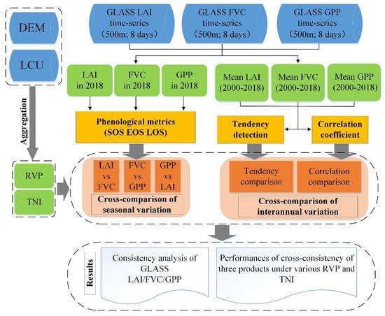
Figure 1.
Flowchart of the comparison scheme for GLASS LAI/FVC/GPP from 2000 to 2018 in the TRSR. All abbreviations are mentioned in the text for the first time.
2.1. Study Area
The TRSR is located between 31°39′–36°16′N and 89°24′–102°23′E and lies in the hinterland of the Qinghai–Tibet Plateau in China (Figure 2) [9]. It includes 22 counties (e.g., Gonghe, Xinghai, Maduo, etc.) and its area is more than 369,000 km2. The TRSR shows complex terrain and heterogeneous land-cover characteristics, and grasslands are the main vegetation type, covering the majority of the study area. The TRSR is widely known as the “Water Tower of China” because it offers 25%, 49%, and 15% of the water for the Yangtze River, Yellow River, and Lancang River, respectively. The TRSR has a representative continental climate, with a small difference in annual temperature and a large difference in diurnal, hydrothermal conditions increasing from northwest to southeast. In the past decades, the TRSR has attracted noticeable attention because it experienced marked climatic changes, e.g., significant increases in rainfall, temperature, and solar radiation. Moreover, the ecogeological environment security of the TRSR, and even the Southeast Asia region, is facing a dangerous situation with the deteriorative regional ecosystem and a decrease in water conservation function.
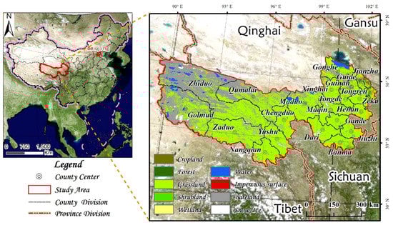
Figure 2.
Study area. The land-cover maps in the right panel were published by Gong et al. [34].
2.2. Datasets
All the GLASS products were obtained from the Nation Earth System Data Center, National Science & Technology Infrastructure of China (http://www.geodata.cn, accessed on 20 November 2021). Table 1 shows the product information. All the GLASS products were firstly transformed from HDF to GeoTIFF format and then reprojected from the sinusoidal to the AEA_WGS_1984 projection. Subsequently, the average composition method was used to achieve the temporal GLASS datasets during the period of 2000 to 2018 growing seasons.

Table 1.
GLASS products were investigated in the study.
2.2.1. GLASS LAI
The GLASS LAI was calculated from the MOD09A1 using a general regression neural network (GRNN) method at a global scale with spatial and temporal resolutions of 8-day and 500 m, respectively [10]. The “effective” CYCLOPES LAI was firstly converted to the actual value using the clumping index (Ω), using the following equation:
Then, the MODIS and CYCLOPES LAI were fused in a weighted linear combination to obtain the best LAI estimate. The MOD09A1 data were reprocessed to clear cloud barrier, and the missing gaps were filled to obtain spatial–temporal continuous and smooth data using the algorithm proposed by Tang et al. [35]. A GRNN was trained using the fused LAI for each biome type and the MOD09A1 data over the Benchmark Land Multisite Analysis and Intercomparison of Products (BELMANIP) sites. Ultimately, the annual LAI profiles were retrieved using the neural network trained from the MOD09A1 reflectance data [10].
2.2.2. GLASS FVC
The GLASS FVC [12,13] was firstly generated by selecting a global sampling location based on the BELMANIP sites, and high-quality Landsat TM/ETM+ data were employed at each site to generate high spatial resolution FVC samples. Subsequently, Landsat data were preprocessed using global land-cover data with 30 m resolution and global terrestrial ecoregion, and the FVC was estimated using a dichotomous pixel model. In addition, the MODIS surface reflectance data were reprocessed to eliminate cloud contamination and other effects.
Based on the global high-resolution FVC sample dataset, four machine learning methods, namely back-propagation neural networks, GRNNs, support vector regression, and multivariate adaptive regression splines (MARS), were evaluated to generate GLASS FVC. All four machine learning methods were trained using sample data from the same sampling location and by comparing their fitting accuracy and computational efficiency; the MARS model was then selected as the most suitable method. Finally, the MARS was trained and used to estimate the global surface FVC [14].
2.2.3. GLASS GPP
GLASS GPP products were produced using a revised eddy covariance light-use efficiency (EC-LUE) model, integrated by the following variables: atmospheric CO2 concentration, radiation components, and atmospheric water vapor pressure [15,33]. The algorithm considered the effects of saturation water vapor pressure deficits, atmospheric CO2 concentrations, and long-term changes in radiation. In addition, the development and validation of the algorithm were based on global eddy flux towers data which includes 84 sites; it covers nine terrestrial ecosystem types: evergreen broadleaf forest, evergreen needleleaf forest, deciduous broadleaf forest, mixed forest, grasslands, savannas, shrubs, wetlands, croplands, etc. The revised model could interpret 68% and 83% of the spatial variations in the annual GPP at 43 validation and 42 calibration sites, respectively. Hence, the estimated GPP derived from the revised EC-LUE model provides an alternative and reliable dataset at the long-term scale by integrating the important environmental variables.
2.2.4. Ancillary Data
Land-Cover Data
The global land-cover maps with 30 m spatial resolution were made using Landsat time-series data [34]. An exclusive land-cover classification system was developed that contains ten primary biomes (e.g., cropland, forest, grassland, shrubland, wetland, water, tundra, impervious surface, bare land, and snow/ice). The first five biomes are considered as vegetation type pixels and other species are considered as nonvegetation type pixels. Subsequently, the ratio of vegetation pixels (RVP) [36] is calculated by using the spatial aggregation method under a 500 m spatial resolution grid, which reflects the LCH characteristic more comprehensively.
DEM Data
The terrain data were derived from the Advanced Spaceborne Thermal Emission and Reflection Radiometer Global Digital Elevation Model Version 2 (ASTER-GDEM V2) with a spatial resolution of 30 m. To reflect the complexity of the topographic features in the TRSR, this study introduces the terrain niche index (TNI) [37] with the following equation:
where is the TNI; and represent the elevation with 30 m spatial resolution and the elevation aggregated to 500 m resolution using the spatial averaging method, respectively. Similarly, and perform the slope with 30 m and 500 m spatial resolution, respectively. By employing the above equation, the original topographic properties (i.e., elevation and slope) can be described by TNI. The areas with low TNI values represent low elevations and flat terrains, and the areas with high TNI values indicate high elevations and sloping terrains, whereas regions with middle TNI values mean the other cases.
The terrain and land-cover data were firstly projected, mosaicked, and aggregated to match the GLASS grid, then terrain and surface heterogeneity metrics were extracted based on a 500 m grid by using zonal statistics. Subsequently, the RVP metrics were then divided into 10 (0–10%, 10–20%, …, 90–100%) groups based on an interval of 10% (Figure 3a). Similarly, the TNI was divided into 12 groups (0–0.2, 0.2–0.4, …, >2.2) based on an interval of 0.2 (Figure 3b).
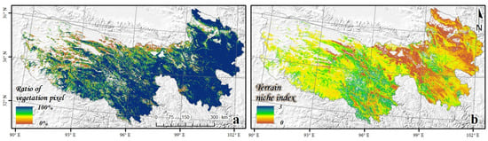
Figure 3.
Ancillary data: (a) Pixel ratio map of vegetation; (b) Terrain niche index.
2.3. Research Methods
Comparison analyses of correlation [38] and trend [19] were effective methods to evaluate the time series performances of different products. In this study, simple and robust Theil–Sen’s slope estimator [39], Mann–Kendall test [40], and Spearman correlation coefficients [41] were used to reflect the interannual consistency of change direction and correlation among different products. Besides, Xia et al. [42] reported that, compared with other models, the phenological metrics derived from the double-logistic function had the highest accuracy. Hence, the LSP extracted by fitting the double-logistic regression function was used in this study to explore the seasonal characteristics among different products.
2.3.1. Phenological Metrics
Several important LSP metrics can be inferred from the LAI/FVC/GPP annual profiles, e.g., the SOS, the EOS, etc. These metrics represent the ecological responses of vegetation communities to environmental variations over spaces and times and define the key phenological phases of vegetation dynamics at annual time scales, which are often used in remote sensing-based phenology studies [43,44,45,46].
Here, we employ a double logistic regression function to reconstruct the annual vegetation growth curve [47]. Based on this function, it is possible to systematically determine the phenological metrics at regional, or even larger, scales. The smooth temporal profile in LAI/FVC/GPP data for a whole year can be modeled using a function of the following form:
where is time in the DOY; is the observed LAI/FVC/GPP at the DOY; is the background value; is the difference between the early summer plateau and amplitude of spring; and is the difference between the background and the amplitude of the summer and autumn plateau; and represent normalized slope coefficients of spring and fall, respectively; and perform the midpoints in DOY of transitions for the greening and browning, respectively.
LSP metrics can be scientifically calculated by the reconstructed temporal trajectories. We investigated and compared the SOS and EOS indicators inferred from three products in 2018, respectively. The SOS and EOS correspond to the DOY of the local maxima and minima of the first derivatives of the fitted curve, respectively.
2.3.2. Trend Detection
Temporal trends of each product are calculated by employing Theil–Sen’s slope estimator with time as the independent variable and remote sensing data as the dependent variable. This method is insensitive to outliers, so it is more robust, theoretically. We used the modified Z-score to standardize the raw data before calculated the trend. The formula of Theil–Sen’s slope estimator is as follows:
where Median is a statistic function; Xj and Xi are the biophysical data, and β indicates the indicates the trends for each pixel. The determination of the significance level is supplemented by the Mann–Kendall test. The algorithms are as follows:
where sgn is the symbolic function; n represents the number of years during 2000–2018, i.e., n = 19. The standard normal test statistic (Z) can be calculated by
where var indicates the variance; m is the number of recurring datasets in the series, and ti is the number of repeated datasets in the i group.
The outputs of the Theil–Sen analysis and Mann–Kendall test are two images of the slope and significance tests at the 500 m resolution. When |Z|> Z1−α/2, the null hypothesis is refuted, and the trend is significant. The value of Z1−α/2 can be found in the standard normal distribution table. In this research, significance degree at α = 0.05 is selected, which corresponded to Z1−α/2 value of 1.96 to classify the slope values into three categories: significant positive (β > 0, |Z| > 1.96), negative (β < 0, |Z| > 1.96), and insignificant changes (β ∃, |Z| ≤ 1.96) [19,48].
2.3.3. Correlation Coefficient
The Spearman rho correlation coefficient is used to determine the level of correlation between every two variables and is usually represented as r-values [49]. It is a nonparametric factor that estimates the dependence between the rankings of two products. If there are no repeated values in the data and the two variables are perfectly monotonically correlated, the Spearman correlation coefficient is either −1 or +1, with the former representing a completely negative correlation and the latter a totally positive correlation. The correlation r of each two variables is calculated by the following equation:
where A and B represent the different products used in this research, respectively. d is the discrepancies between the ranks of two products, and n is the length of each observation, i.e., n = 19. The output r-values indicate the correlation coefficient between the two products from 2000 to 2018.
Significance tests are selected at a level of α = 0.05 to classify the correlation types into three categories: positive correlation (r > 0, α < 0.05), negative correlation (r < 0, α < 0.05), and insignificant correlation (r∃, α > 0.05) [50,51]. The formula of significance test is shown in [52].
2.3.4. Comprehensive Assessment Framework
To comprehensively evaluate the performances among GLASS products, the agreement level of LSP metrics was firstly estimated by calculating their absolute difference (days). In addition, the results of the long-term trend analysis and correlation detection were counted and used to populate the comparisons framework, as framed in Figure 4. This framework was used to assess the matching degree of interannual variation among three products. Physical agreement situations were assumed as the following forms (Figure 4):
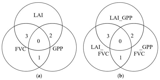
Figure 4.
Comparison framework of (a) tendency and (b) correlation among three products.
- The pixels with ID 0 indicate that all products are agreed in the trend comparison, i.e., consistently positive, negative, or insignificant changes; while in the correlation comparison, it means that three datasets are synchronously positively, negatively, or insignificantly correlated between each other.
- In the tendency comparison, the pixels with ID 1 represent FVC and GPP agreement in positive, negative, or insignificant changes, while LAI disagrees with the other two products. In the correlation comparison, the pixels with ID 1 indicate FVC has a consistently positive, negative, or insignificant relationship with LAI or GPP, while LAI and GPP are oppositely correlated.
- The pixels with ID 2 indicate that GPP and LAI have the same trend direction in these areas (i.e., positive, negative, or insignificant changes), however, FVC is inconsistent; while in the correlation comparison, it means that GPP has the same positive, negative, or insignificant relationship between FVC or LAI, but the correlation between FVC and LAI is reversed in these regions.
- The pixels with ID 3 intend that LAI and FVC agree (i.e., accordant positive, negative, or insignificant changes), nevertheless, GPP disagrees in the tendency directions; while in correlation comparison, it means that LAI has the same positive, negative, or insignificant correlation between FVC or GPP, while the correlation between GPP and FVC is opposite.
In summary, pixels with ID 0 represent that the interannual trend and correlation are in total agreement in comparison, and pixels with ID 1, 2, and 3 indicate the total disagreement (i.e., interannual differences). Subsequently, the statistical distributions of comparison results of LSP and interannual variation as a function of the RVP and TNI indicators, respectively, are calculated to reveal the performances of temporal agreements among LAI/FVC/GPP under different characteristics of TC and LCH.
3. Results
3.1. LSP Characteristics of Three Products
3.1.1. Spatial Patterns of LSP of LAI/FVC/GPP
Using the LAI/FVC/GPP data in 2018, we display the spatial patterns of the LSP in the TRSR (Figure 5). In general, the patterns are elevation-dependent, and vegetation growth in northwestern parts of the study areas (i.e., Zhiduo, Qumalai, and Golmud counties) occurs a little later than the other areas. Most pixels’ SOS there begin after 135 DOY, while EOS happen before 275 DOY. Eastward from the Zhiduo county, the SOS advances from May to April, and the EOS postpones from September to October. In other words, with the increasing elevation in the TRSR, the SOS delays from the southeast to northwest, while EOS is in advancement.
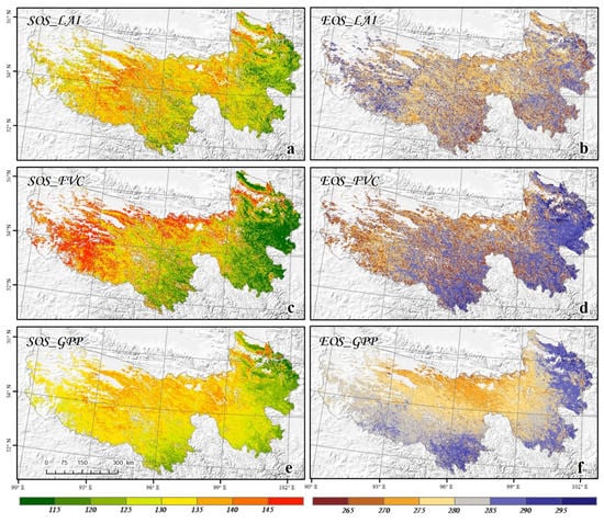
Figure 5.
Spatial patterns of the land surface phenology derived from (a,b) LAI, (c,d) FVC, and (e,f) GPP in 2018 across TRSR. The left panels display the start of the growing season, and the right panels show the end of the growing season.
Despite the similar spatial pattern exhibited by the three various products, there are still noteworthy variances in the estimation of LSP metrics from different products (Table 2). In the estimations of SOS, 42.22% and 39.80% of the pixels indicate that the phenological differences of LAI_FVC and FVC_GPP are more than 10 days; while in the EOS estimates, these percentages are 41.92% and 32.62%, respectively. In brief, at least 35% of the pixels in the study area represent a significant difference between FVC and other products in LSP estimation, which are mainly located at the Golmud, Zhiduo, Qumalai, and Gonghe counties. However, 95.38% and 85.50% of the pixels prove that the phenological differences between GPP and LAI are within 10 days, respectively. This phenomenon implies that the LSP estimations by GPP and LAI enjoy better agreements in the vast majority of the study area (more than 90%).
Table 2.
The statistical distribution of absolute difference (days) of SOS and EOS between every two products.
3.1.2. Performances of Phenological Differences among LAI/FVC/GPP under Different Surface Conditions
The left and right panels in Figure 6 show the variation of phenological differences (days) of SOS and EOS varying with RVP and TNI across TRSR, respectively. A clear phenomenon can be derived in which the discrepancies of phenological indicators decrease with the increase of RVP (the left panels). The minimum phenological differences are simultaneously observed over the regions with homogeneous land cover (i.e., RVP level larger than 80%), the maximum, conversely, are captured at the heterogeneous surfaces (i.e., RVP level less than 30%). Note that the differences of SOS derived from LAI and FVC products can reach about 10 days between the most homogeneous and heterogeneous surfaces (panel a). This further illustrates that LSP retrievals from three products show poor performances under heterogeneous surfaces.
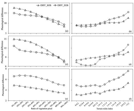
Figure 6.
Phenological difference (days) between (a,b) LAI and FVC, (c,d) FVC and GPP, and (e,f) GPP and LAI, varying with the ratio of vegetation pixel (left panels) and terrain niche index (right panels) in 2018 across TRSR.
The absolute discrepancies of phenological metrics between every two products increase with rising TNI (the right panels), which firstly remains relatively stable at the 0–1.0 level and then increases rapidly at the >1.0 level. Overall, the discrepancies at high altitudes with rugged surfaces are larger than those at low elevations with flat terrain, regardless of SOS and EOS. This suggests that the agreements of LSP metrics derived from three products under the areas with high TNI values exhibit poor performances.
3.2. Long-Term Characteristics of Three Products
3.2.1. Tendency and Correlation of LAI/FVC/GPP
The left panels in Figure 7 present spatial distributions of vegetation change trends by employing the Theil–Sen’s slope estimator. Note that the Mann–Kendall test not marked in the panel. All datasets generally display a large area of significant positive trends in the northeastern (e.g., Gonghe, Jianzha, Guide, Guinan counties, etc.) and northwest TRSR (e.g., Zhiduo and Golmud counties). A few pixels with negative trends among three products have been found in the northwestern and southern TRSR.
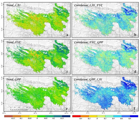
Figure 7.
Spatial patterns of the slope values estimated from Theil–Sen trend analysis of LAI (a), FVC (c), and GPP (e), and the r-values estimated from Spearman rank correlation coefficient analysis between LAI_FVC (b), FVC_GPP (d), and GPP_LAI (f) during 2000–2018 across the TRSR.
Table 3 shows the statistical results of the change trends of three products from the 2000 to 2018 growing season. A significant tendency is observed for 10.44% of the LAI pixels, including 5.63% positive trends and 4.81% negative trends, whereas the FVC analysis generates approximately 19.92% significant pixels (17.37% and 2.55% with positive or negative trends, respectively). In addition, the GPP produces about 5.47% significant pixels (5.31% positive and 0.16% negative).
Table 3.
Statistical results on the correlations and trends of LAI, FVC, and GPP products during 2000–2018 (α = 0.05).
The right panels in Figure 7 show the correlation between each of the two products using the Spearman rank correlation coefficient method from 2000 to 2018 growing seasons in the TRSR. The highly positive relationship pixels among all datasets have been found in the northeastern TRSR (e.g., Gonghe, Guide, Jianzha, Guinan, Xinghai counties, etc.), and northern or northwestern TRSR (e.g., Maduo, Qumalai counties, etc.). Conversely, there were a few negative pixels found in the Golmud, Nangqian, Yushu counties, etc. As far as the statistical result was concerned, the proportion of positive correlation pixels between GPP and LAI is 74.59%, while FVC~GPP and LAI~FVC is 34.70% and 42.52%, respectively (Table 3).
3.2.2. Comprehensive Assessment of Long-Term Changes in LAI/FVC/GPP
Figure 8 presents the trend comparison map of LAI, FVC, and GPP, at a per-pixel level. The dark green and dark red pixels (i.e., ID 0) represent the three products showing consistent positive and negative trend directions, respectively. The agreed positive tendency among three datasets is unambiguous across most of the northeastern (e.g., Jianzha, Guide, Tongren counties, etc.) and part of the northwestern TRSR (e.g., Zhiduo and Golmud counties). A few agreed positive pixels were also found in the western part of Dari County. In addition, the areas of agreed negative are usually concentrated in the northern TRSR (e.g., Qumalai county) and parts of the southeastern TRSR (e.g., Dari and Gande counties).
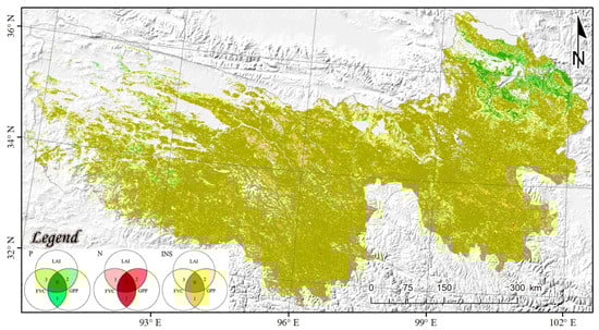
Figure 8.
Spatial patterns of long-term trend comparison estimated from LAI, FVC, and GPP during the 2000–2018 growing season across the TRSR. The dark-colored pixels with ID 0 represent total agreement in the trend direction, i.e., total agreed in positive (P0), negative (N0), and insignificant changes (INS0), while light-colored pixels with ID 1, 2, or 3 represent total disagreement, i.e., total disagreed in positive (P1, P2, or P3), negative (N1, N2, or N3), and insignificant changes (INS1, INS2, or INS3), and the meanings of each ID are shown in Section 2.3.4.
Table 4 displays the statistical information of the metrics of interannual consistency derived from trend analysis. The trend direction of all datasets agrees in 76.08% of the whole TRSR, collectively displaying agreement with positive tendencies of 2.50% and very few negative tendencies of 0.06%. The light-colored pixels (i.e., ID 1, 2, and 3) indicate regions where two out of three products synchronously display a positive, negative, or insignificant trend, while the third product exhibits an inconsistent tendency. In this region, FVC most often shows an inconsonant tendency where the other two products show an accordant trend direction. The pixels with ID 2 accounts for about 13.96% of the whole TRSR. Conversely, LAI (i.e., the pixels with ID 1) and, to a lesser extent, GPP (i.e., the pixels with ID 3), show relatively few inconsistencies for 6.15% and 3.81% pixels, respectively.
Table 4.
Comparison statistics of the agreement metrics of interannual variation difference, derived from three products.
Figure 9 depicts the correlation comparison map derived from the Spearman correlation analysis by LAI, FVC, and GPP from the 2000 to 2018 growing season. The pixels with ID 0 indicate a consistent positive or negative correlation for three products. Accordantly, positive correlations among all products are obviously across the majority area of the northeastern (e.g., Gonghe, Jianzha, Guide counties) and northwestern (e.g., Golmud county) TRSR. In addition, there are a few consistently positively correlated pixels found in the northern parts of the study area (e.g., Maduo county).
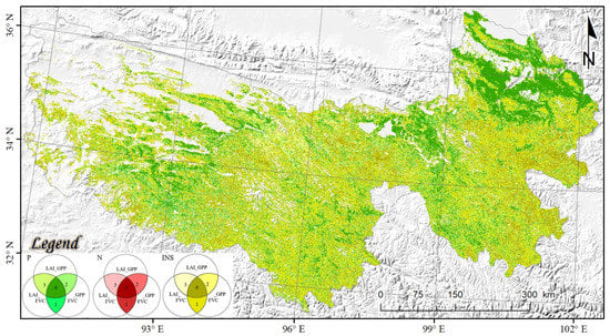
Figure 9.
Spatial patterns of long-term correlation comparison calculated by LAI, FVC, and GPP during the 2000–2018 growing season across the TRSR. The dark-colored pixels with ID 0 represent total agreement in the correlation, i.e., total agreement in positive (P0), negative (N0), and insignificant correlation (INS0), while light-colored pixels with ID 1, 2, or 3 represent total disagreement, i.e., total discordant in positive (P1, P2, or P3), negative (N1, N2, or N3), and insignificant correlation (INS1, INS2, or INS3), and the meanings of each ID are shown in Section 2.3.4.
Table 4 shows the statistical results of the interannual correlated comparison derived from the correlation analysis. The rank relation among all datasets agrees in 38.96% across the whole TRSR, respectively, revealing a positive correlation of 23.08% and a negative correlation of less than 0.01%. The percentages of light-colored pixels with ID 1, 2, and 3 describe the extent to which FVC, GPP, and LAI are inconsistent with the other two products, respectively. For example, the pixels with INS1 show the ratio of 31.80% in the whole TRSR, which means that GPP is significantly correlated with LAI in these regions, while FVC is not significantly correlated with both products. As far as the proportions of light-colored pixels with ID 1, 2, or 3 are concerned (i.e., total disagreement), these account for 33.24%, 12.74%, or 15.06%, respectively, that is, FVC is the most inconsistent with the other two products in the correlation comparison.
3.2.3. Performances of Long-Term Variations among LAI/FVC/GPP under Various Situations
Figure 10 illustrates the performances of comparison of interannual variations among three products over different degrees of RVP and TNI. As far as the comparison of long-term trends is concerned (panels a and b in Figure 10), the total agreement tends to decline (or rise) with increasing RVP (or TNI), and it seems that the long-term trends of the three products have “good” performances over the areas with high heterogeneous surfaces or complex terrain. Nevertheless, after separating the agreed positive changes (P0) from the total agreement, an explicit differentiation pattern shows that the P0 tends to decrease with the rising TNI (panel c) and increase with the ascending RVP (panel d). The INS0, conversely, raises with the increasing TNI and declines with the increasing RVP (not marked in the panel). This phenomenon indicates that the long-term trends of the three products show poor performances under heterogeneous surfaces or complex terrain.
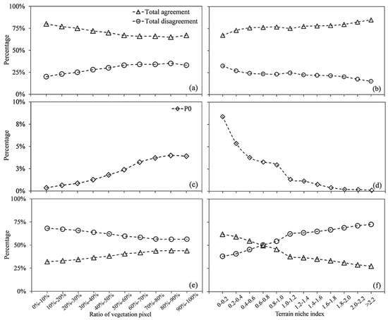
Figure 10.
The statistical distribution of comprehensive assessment results of the tendency (a,b) and correlation (e,f) of three products varying with the ratio of vegetation pixel and terrain niche index. The statistical distribution of agreed positive trends (P0) calculated by LAI, FVC, and GPP varying with the ratio of vegetation pixel (c) and terrain niche index (d).
Panels e and f in Figure 10 depict the performances of interannual correlation comparison of the three products under different levels of RVP and TNI. A clear statistical distribution suggests that the percentage of total agreement tends to be decreasing with increasing land-cover heterogeneity (RVP) or surface complexity (TNI), which indicates the long-term correlations of the three products, also showing poor performances under heterogeneous ground surfaces or complicated topography.
4. Discussions
4.1. Importance of Comprehensive Assessment for Biophysical Products
In this study, double-logistic function, Theil–Sen’s slope estimator, Mann–Kendall test, and Spearman correlation coefficient were employed to examine the LSP and long-term changes of vegetation of LAI, FVC, and GPP from 2000 to 2018 in the TRSR. Most previous research for estimating vegetation tendency or phenological phases has been based on the employment of vegetation indices. Yet, vegetation indices were greatly different in the LSP estimations over specific spaces and various vegetation types [8]. Biophysical variables were more sensitive than vegetation indices to dense vegetation. This was particularly significant to describe the later phases of canopy growth and leaf maturity. In addition, phenological and interannual tendency estimations were also expected to be more robust across different biophysical data than those in vegetation indices, because vegetation indices highly depend on the band characteristics across various sensors [23]. It was also reported that the high discordances in the characteristics of seasonal patterns between various vegetation indices and MODIS datasets, and vegetation indices seasonality still lacks a robust biophysical explanation across the Amazon rainforest [53]. It further highlighted the shortcomings of vegetation indices and the ecological significance of synergistic employment of biophysical products for time-series analysis.
Nevertheless, previous researchers directly apply a single product to analyze vegetation dynamics or LSP, which often leads to contradictory conclusions in special cases [48]. Moreover, a comparative study on the time-series performance of different biophysical products can also improve the cognition of the uncertainty of land surface models. Given that these products are often combined with various satellite data as input parameters into the land surface models, the credibility of results is crucial for users when GLASS products are assimilated together into a land surface model. Therefore, the systematic and reliable identification of phenology and interannual variations of surface vegetation using multiple GLASS products at large spatiotemporal scales is of great significance to clarify the patterns of spatial and temporal processes in typical mountain areas, and these activities can also promote the effective deployment of sustainable management strategies for mountain ecosystems.
4.2. Mismatches of Long-Term Variations and LSP among LAI/FVC/GPP
We find a significant positive tendency on surface vegetation over the northeastern and northwestern TRSR during the last 20 years, which is consistent with one recent study [9]. However, there exists a large mismatch between FVC with other two products, regardless of LSP detection, interannual trend, and correlation. These phenomena may be caused by the influences of combinations of various factors, such as the algorithms and effects of climate or other environmental factors.
Firstly, all these biophysical variables are typical indicators used to characterize the growth status of green vegetation; FVC and LAI can also be linked by the Beer–Lambert equation, theoretically [54,55]. Yet, FVC is not a proxy of LAI or GPP, as environment and human activities may restrain the process of green vegetation carbon sequestration over a long period. A recent study conducted in the Amur River basin also indicates a much weaker rise in GPP growth rate when compared with the FVC, partly due to the influences of environmental factors (e.g., warming-induced drying) [3]. In addition, current retrieval algorithms of those products are mostly designed to acquire a single variable from remote sensing observations. Thus, various parameters are retrieved from different models and schemes based on various physical assumptions [56]. These parameter-specific approaches ignore the physical connections between the various datasets, resulting in a difference among different time-series biophysical products even if they are estimated from the same remote sensing data. Lastly, we observe good agreements between LAI and GPP in the TRSR. The reason may be explained by LAI having significant effects on the GPP estimations in the revised EC-LUE model [33,57]. More specifically, the absorbed photosynthetically active radiation (APAR) by green leaves is an important parameter in the revised EC-LUE model, while LAI is critical in the calculation of APAR.
Note that we find the LSP metrics and long-term changes of the three products perform better on homogeneous surfaces (i.e., high RVP level) and flat terrain (i.e., low TNI level). This phenomenon may be explained by the fact that the pixels with high RVP or TNI values are usually located at high altitudes in the TRSR, and the climatic warming-induced drying may significantly affect vegetation growth and carbon uptake at high elevations [20]. In addition, the estimation of vegetation phenology at the pixel level remains a large uncertainty and can reach approximately ±20 days, especially in high-elevation areas [44]. Both the effects of species composition [45] and the frequency and mixture of species present in each pixel [46] contribute to high variability in phenological estimations. More specifically, the spatial resolution of satellite products used in our study is 500 m, and the pixels are generally not composed of a homogeneous ground biome type, but a mixture of several classes. The pixels, therefore, are not a single but mixed reflections of spectral features of several ground communities [58]. The heterogeneous pixels may have a significant negative effect on the accurate retrieval of global biophysical products, whereas the current algorithms of GLASS products do not consider the mixed characteristics of pixels.
On the other hand, the quality of satellite products becomes poor as the topographic complexity increases. Firstly, local topography may cause the frequent occurrence of climate change so that reflectance data in these regions often receive contaminations from aerosols, clouds, and snow [59]. Fortunately, the surface reflectance data are reprocessed to remove the influences of extreme climatic change before inputting the algorithm [35]. The rugged surfaces also influence the irradiance and bidirectional reflectance distribution function (BRDF) of optical satellite images [60]. Significant differences exist in the solar irradiance received by areas with different slopes. Furthermore, the rugged surfaces result in the raised angular variations between the satellite sensors and the sun, which may further increase the complexity of BRDF and bring high uncertainties in data quality [61].
Overall, the LSP and long-term variations inferred from LAI, FVC, and GPP display strong spatial heterogeneity with diverse spatial patterns, especially at high altitudes in the TRSR. Commonly, this phenomenon is the comprehensive consequence of climate stress, anthropogenic influence, and differences of retrieval algorithms for different products. The mechanisms behind this phenomenon need further research to better understand and improve the predictions of mountain vegetation activity under different climate scenarios in the future.
4.3. Limitations and Prospects
As far as we know, this study is the first to analyze the performances of different biophysical products in the TRSR region both in terms of LSP detection and long-term changes; however, it must be emphasized that the regression model and Spearman correlation coefficient used in this study are statistical analyses, whereas statistical analyses are methods to objectively calculate the linear relationship between time variables and vegetation growth. Several studies [62,63] give evidence that the correlations and responding mechanisms between ecosystem and natural variation are nonlinear, which highlights the potential defect of linear statistical analysis. This limitation may be overcome by correctly and appropriately adopting process-based ecosystem models in further studies.
Our study also indicates the high mismatch of LSP metrics observed in areas with highly rugged surfaces or landscape fragmentations. Given the highly surface heterogeneity and topographic complexity, the inversion accuracy of GLASS products should be enhanced. Particularly, the high uncertainties of surface reflectance data limit latent development of the algorithms of biophysical products, and subsequently influence the performance of LSP retrievals of GLASS products over mountain areas. The improvement of retrieval algorithms with topography and heterogeneous surface in consideration will help to improve the inversion accuracy [32]. Furthermore, coarse-resolution pixels will greatly increase the uncertainties of spectral information, which would propagate into the production of global products. Paradoxical conclusions may arise from integrated analysis by end-users using multiple time-series satellite products, which poses a challenge for reliable monitoring and attribution in LSP and vegetation dynamics over some special environments. Thus, it is an imminent study to develop various satellite products with finer resolution (e.g., 30 m or even higher) over heterogeneous surfaces and complex terrains.
Overall, the disproportionate increase between vegetation greening trend, represented by FVC, with vegetation carbon sequestration indicates that the climatic conditions and human activities in the TRSR may hinder the conversion of vegetation greening to a carbon sink. Therefore, we emphasize that the existing natural vegetation in the TRSR needs to be further protected. The time-series analysis based on a single product may not be directly considered as a convincing result when exploring the long-term changes of vegetation, carbon, and water cycles in the TRSR. Hence, we propose the application of a complementary combination of simulation data based on climate and human impacts with multiple products as a new attempt for tendency analysis, which may greatly improve the interpretation and attribution of vegetation trends.
5. Conclusions
In this study, the time-series characteristics of three GLASS products (LAI, FVC, and GPP) were assessed based on the tendency, correlation, and phenological retrieval methods during 2000 to 2018 in the TRSR. Moreover, the performances of these products over different surfaces and terrain were analyzed. We found that three products reasonably displayed the vegetation phenological characteristics and their interannual variations across TRSR. Nevertheless, the phenological differences between FVC and two other products were larger than 10 days in more than 35% of pixels in the study area, and the proportion of large differences of LSP between GPP and LAI was only 10%. Moreover, we proved that the long temporal variations of FVC were significantly different from LAI and GPP in the TRSR from 2000 to 2018. The significant positive trends of LAI and GPP (~5%) were much weaker than those in the FVC (~17%). Note that the poor performances of LSP metrics and long-term changes were observed at the regions with heterogeneous land cover (i.e., low RVP level) and rugged surfaces (i.e., high TNI level). This demonstrates that the complex effects of both the algorithm and the environmental factors at high elevation can cause a high degree of difference in the time-series performances of different products.
In brief, this research highlights the potentiality of joint application of GLASS products for observing vegetation characteristics and regional carbon dynamics in mountainous areas. The intercomparison of different time-series products is crucial for not only the recognition of the relationship between vegetation greening and the carbon cycle in mountainous areas, but also the refinement of the retrieval algorithm of global products over mountain areas. In the future, we will evaluate the performance of various biophysical products with high spatial resolution and utilize the process-based models to assess vegetation dynamics at global or regional scales.
Author Contributions
Conceptualization, H.J., H.S. and W.Z.; methodology, H.J., H.S. and W.Z.; software, G.L., X.N. and X.X.; writing—original draft preparation, W.Z. and W.F.; writing—review and editing, H.J., A.L. and H.S.; visualization, W.Z. and G.H.; supervision, H.J., A.L. and H.S.; project administration, H.J. and A.L.; funding acquisition, H.J. and A.L. All authors have read and agreed to the published version of the manuscript.
Funding
This research was funded by National Key Research and Development Program of China (Grant No. 2016YFA0600103), National Natural Science Foundation of China (Grant No. 42071352, 41631180, 41801370), and the Chinese Academy of Sciences (CAS) “Light of West China” Program.
Institutional Review Board Statement
Not applicable.
Informed Consent Statement
Not applicable.
Data Availability Statement
(1) The GLASS products introduced in this paper are available in [http://www.geodata.cn/index.html, accessed on 20 November 2021] or [http://glass.umd.edu/Download.html, accessed on 20 November 2021], reference number [2,3,4,5,6,7]. (2) DEM and land cover data can be found in: [http://www.gscloud.cn/, accessed on 20 November 2021] or [http://data.ess.tsinghua.edu.cn/, accessed on 20 November 2021], reference number [35].
Acknowledgments
The authors would like to thank teachers and work fellows of the Research Center for Digital Mountain and Remote Sensing Application, Institute of Mountain Hazards and Environment for their support during this research. Meanwhile, we thank all members of Shunlin Liang’s team providing the GLASS products for us. In addition, we are also most thankful to the anonymous reviewers and all the editors for their helpful comments and suggestions.
Conflicts of Interest
The authors declare no conflict of interest.
References
- Guo, X.; Zhang, H.; Wu, Z.; Zhao, J.; Zhang, Z. Comparison and Evaluation of Annual NDVI Time Series in China Derived from the NOAA AVHRR LTDR and Terra MODIS MOD13C1 Products. Sensors 2017, 17, 1298. [Google Scholar] [CrossRef] [Green Version]
- Peng, D.; Wu, C.; Zhang, X.; Yu, L.; Huete, A.R.; Wang, F.; Luo, S.; Liu, X.; Zhang, H. Scaling up spring phenology derived from remote sensing images. Agric. For. Meteorol. 2018, 256–257, 207–219. [Google Scholar] [CrossRef]
- Zhou, S.; Zhang, W.; Wang, S.; Zhang, B.; Xu, Q. Spatial–Temporal Vegetation Dynamics and Their Relationships with Climatic, Anthropogenic, and Hydrological Factors in the Amur River Basin. Remote Sens. 2021, 13, 684. [Google Scholar] [CrossRef]
- Wen, Z.; Wu, S.; Chen, J.; Lu, M. NDVI indicated long-term interannual changes in vegetation activities and their responses to climatic and anthropogenic factors in the Three Gorges Reservoir Region, China. Sci. Total Environ. 2017, 574, 947–959. [Google Scholar] [CrossRef]
- Mao, D.; Wang, Z.; Luo, L.; Ren, C. Integrating AVHRR and MODIS data to monitor NDVI changes and their relationships with climatic parameters in Northeast China. Int. J. Appl. Earth Obs. Geoinf. 2012, 18, 528–536. [Google Scholar] [CrossRef]
- Wu, C.; Peng, D.; Soudani, K.; Siebicke, L.; Gough, C.M.; Arain, M.A.; Bohrer, G.; Lafleur, P.M.; Peichl, M.; Gonsamo, A.; et al. Land surface phenology derived from normalized difference vegetation index (NDVI) at global FLUXNET sites. Agric. For. Meteorol. 2017, 233, 182. [Google Scholar] [CrossRef]
- Wu, C.; Gonsamo, A.; Gough, C.M.; Chen, J.M.; Xu, S. Modeling growing season phenology in North American forests using seasonal mean vegetation indices from MODIS. Remote Sens. Environ. 2014, 147, 79–88. [Google Scholar] [CrossRef]
- Peng, D.; Wu, C.; Li, C.; Zhang, X.; Liu, Z.; Ye, H.; Luo, S.; Liu, X.; Hu, Y.; Fang, B. Spring green-up phenology products derived from MODIS NDVI and EVI: Intercomparison, interpretation and validation using National Phenology Network and AmeriFlux observations. Ecol. Indic. 2017, 77, 323–336. [Google Scholar] [CrossRef]
- Zhang, W.; Jin, H.; Shao, H.; Li, A.; Li, S.; Fan, W. Temporal and Spatial Variations in the Leaf Area Index and Its Response to Topography in the Three-River Source Region, China from 2000 to 2017. ISPRS Int. J. Geo-Inf. 2021, 10, 33. [Google Scholar] [CrossRef]
- Xiao, Z.; Liang, S.; Wang, J.; Chen, P.; Yin, X.; Zhang, L.; Song, J. Use of General Regression Neural Networks for Generating the GLASS Leaf Area Index Product From Time-Series MODIS Surface Reflectance. IEEE Trans. Geosci. Remote Sens. 2014, 52, 209–223. [Google Scholar] [CrossRef]
- Xiao, Z.; Liang, S.; Wang, J.; Xiang, Y.; Zhao, X.; Song, J. Long-Time-Series Global LAnd Surface Satellite Leaf Area Index Product Derived From MODIS and AVHRR Surface Reflectance. IEEE Trans. Geosci. Remote Sens. 2016, 54, 5301–5318. [Google Scholar] [CrossRef]
- Jia, K.; Liang, S.; Wei, X.; Yao, Y.; Yang, L.; Zhang, X.; Liu, D. Validation of Global LAnd Surface Satellite (GLASS) fractional vegetation cover product from MODIS data in an agricultural region. Remote Sens. Lett. 2018, 9, 847–856. [Google Scholar] [CrossRef]
- Jia, K.; Liang, S.; Liu, S.; Li, Y.; Xiao, Z.; Yao, Y.; Jiang, B.; Zhao, X.; Wang, X.; Xu, S.; et al. Global Land Surface Fractional Vegetation CoverEstimation Using General Regression Neural Networks from MODIS Surface Reflectance. IEEE Trans. Geosci. Remote Sens. 2015, 53, 4787–4796. [Google Scholar] [CrossRef]
- Yang, L.; Jia, K.; Liang, S.; Liu, J.; Wang, X. Comparison of Four Machine Learning Methods for Generating the GLASS Fractional Vegetation Cover Product from MODIS Data. Remote Sens. 2016, 8, 682. [Google Scholar] [CrossRef] [Green Version]
- Yuan, W.; Liu, S.; Yu, G.; Bonnefond, J.M.; Verma, S.B. Global estimates of evapotranspiration and gross primary production based on MODIS and global meterology data. Remote Sens. Environ. 2010, 114, 1416–1431. [Google Scholar] [CrossRef] [Green Version]
- Chen, J.M.; Black, T. Defining leaf area index for non-flat leaves. Plant Cell Environ. 1992, 15, 421–429. [Google Scholar] [CrossRef]
- Xie, X.; Li, A. Development of a topographic-corrected temperature and greenness model (TG) for improving GPP estimation over mountainous areas. Agric. For. Meteorol. 2020, 295, 108193. [Google Scholar] [CrossRef]
- Wang, H.; He, M.; Yan, W.; Ai, J.; Chu, J. Ecosystem vulnerability in the Tianshan Mountains and Tarim Oasis based on remote sensed gross primary productivity. Acta Ecol. Sin. 2021, 41, 1–9. [Google Scholar] [CrossRef]
- Yang, L.; Jia, K.; Liang, S.; Liu, M.; Wei, X.; Yao, Y.; Zhang, X.; Liu, D. Spatio-temporal analysis and uncertainty of fractional vegetation cover change over northern China during 2001–2012 based on multiple vegetation data sets. Remote Sens. 2018, 10, 549. [Google Scholar] [CrossRef] [Green Version]
- Zhang, Y.; Song, C.; Band, L.E.; Sun, G. No Proportional Increase of Terrestrial Gross Carbon Sequestration from the Greening Earth. J. Geophys. Res. Biogeosci. 2019, 124, 2540–2553. [Google Scholar] [CrossRef]
- Sarmah, S.; Singha, M.; Wang, J.; Dong, J.; Deb Burman, P.K.; Goswami, S.; Ge, Y.; Ilyas, S.; Niu, S. Mismatches between vegetation greening and primary productivity trends in South Asia—A satellite evidence. Int. J. Appl. Earth Obs. Geoinf. 2021, 104, 102561. [Google Scholar] [CrossRef]
- Zhang, X.; Liu, L.; Yan, D. Comparisons of Global Land Surface Seasonality and Phenology Derived from AVHRR, MODIS and VIIRS Data. J. Geophys. Res. Biogeosci. 2017, 122, 1506–1525. [Google Scholar] [CrossRef]
- Wang, C.; Li, J.; Liu, Q. Analysis on difference of phenology extracted from EVI and LAI. In Proceedings of the 2017 IEEE International Geoscience and Remote Sensing Symposium (IGARSS), Fort Worth, TX, USA, 23–28 July 2017; pp. 5101–5104. [Google Scholar] [CrossRef]
- Du, J.; Jiaerheng, A.; Zhao, C.; Fang, S.; Liu, W.; Yin, J.; Yuan, X.; Xu, Y.; Shu, J.; He, P. Analysis of vegetation dynamics using GIMMS NDVI3g in the Three-Rivers Headwater Region from 1982 to 2012. Acta Pratacult. Sin. 2016, 25, 1–12. [Google Scholar] [CrossRef]
- Zhang, Y.; Zhang, C.; Wang, Z.; Chen, Y.; Gang, C.; An, R.; Li, J. Vegetation dynamics and its driving forces from climate change and human activities in the Three-River Source Region, China from 1982 to 2012. Sci. Total Environ. 2016, 563, 210–220. [Google Scholar] [CrossRef]
- Shao, Q.; Zhao, Z.; Liu, J.; Fan, J. The characteristics of land cover and macroscopical ecology changes in the source region of three rivers on Qinghai-Tibet Plateau during last 30 years. Geogr. Res. 2010, 29, 1439–1451. [Google Scholar] [CrossRef]
- Xue, B.; Wang, G.; Xiao, J.; Helman, D.; Sun, W.; Wang, J.; Liu, T. Global convergence but regional disparity in the hydrological resilience of ecosystems and watersheds to drought. J. Hydrol. 2020, 591, 125589. [Google Scholar] [CrossRef]
- Xue, B.; Helman, D.; Wang, G.; Xu, C.-Y.; Xiao, J.; Liu, T.; Wang, L.; Li, X.; Duan, L.; Lei, H. The low hydrologic resilience of Asian Water Tower basins to adverse climatic changes. Adv. Water Resour. 2021, 155, 103996. [Google Scholar] [CrossRef]
- Liu, Y.; Wang, J.; Dong, J.; Wang, S.; Ye, H. Variations of Vegetation Phenology Extracted from Remote Sensing Data over the Tibetan Plateau Hinterland during 2000–2014. J. Meteorol. Res. 2020, 34, 786–797. [Google Scholar] [CrossRef]
- Wang, J.; Sun, H.; Xiong, J.; He, D.; Cheng, W.; Ye, C.; Yong, Z.; Huang, X. Dynamics and Drivers of Vegetation Phenology in Three-River Headwaters Region Based on the Google Earth Engine. Remote Sens. 2021, 13, 2528. [Google Scholar] [CrossRef]
- Xiao, Z.; Liang, S.; Jiang, B. Evaluation of four long time-series global leaf area index products. Agric. For. Meteorol. 2017, 246, 218–230. [Google Scholar] [CrossRef]
- Jin, H.; Li, A.; Bian, J.; Nan, X.; Zhao, W.; Zhang, Z.; Yin, G. Intercomparison and validation of MODIS and GLASS leaf area index (LAI) products over mountain areas: A case study in southwestern China. Int. J. Appl. Earth Obs. Geoinf. 2017, 55, 52–67. [Google Scholar] [CrossRef]
- Zheng, Y.; Shen, R.; Wang, Y.; Li, X.; Liu, S.; Liang, S.; Chen, J.; Ju, W.; Zhang, L.; Yuan, W. Improved estimate of global gross primary production for reproducing its long-term variation, 1982–2017. Earth Syst. Sci. Data Discuss. 2020, 12, 2725–2746. [Google Scholar] [CrossRef]
- Gong, P.; Wang, J.; Yu, L.; Zhao, Y.; Zhao, Y.; Liang, L.; Niu, Z.; Huang, X.; Fu, H.; Liu, S.; et al. Finer resolution observation and monitoring of global land cover: First mapping results with Landsat TM and ETM+ data. Int. J. Remote Sens. 2013, 34, 2607–2654. [Google Scholar] [CrossRef] [Green Version]
- Tang, H.; Yu, K.; Hagolle, O.; Jiang, K.; Geng, X.; Zhao, Y. A cloud detection method based on a time series of MODIS surface reflectance images. Int. J. Digit. Earth 2013, 6, 157–171. [Google Scholar] [CrossRef]
- Yu, W.; Li, J.; Liu, Q.; Zeng, Y.; Yin, G.; Zhao, J.; Xu, B. Extraction and Analysis of Land Cover Heterogeneity over China. Adv. Earth Sci. 2016, 31, 1067–1077. [Google Scholar] [CrossRef]
- Yu, H.; Zeng, H.; Jiang, Z. Study on Distribution Characteristics of Landscape Elements along the Terrain Gradient. Sci. Geogr. Sin. 2001, 21, 64–69. [Google Scholar] [CrossRef]
- Fensholt, R.; Proud, S.R. Evaluation of Earth Observation based global long term vegetation trends—Comparing GIMMS and MODIS global NDVI time series. Remote Sens. Environ. 2012, 119, 131–147. [Google Scholar] [CrossRef]
- Sen, P.K. Estimates of the Regression Coefficient Based on Kendall’s Tau. J. Am. Stat. Assoc. 1968, 63, 1379–1389. [Google Scholar] [CrossRef]
- Mann, H.B. Nonparametric Test against Trend. Econometrica 1945, 13, 245–259. [Google Scholar] [CrossRef]
- Spearman, C. The proof and measurement of association between two things. Am. J. Psychol. 1987, 100, 441–471. [Google Scholar] [CrossRef]
- Xia, C.; Li, J.; Liu, Q. Review of advances in vegetation phenology monitoring by remote sensing. J. Remote Sens. 2013, 17, 1–16. [Google Scholar]
- Tong, X.; Tian, F.; Brandt, M.; Liu, Y.; Zhang, W.; Fensholt, R. Trends of land surface phenology derived from passive microwave and optical remote sensing systems and associated drivers across the dry tropics 1992–2012. Remote Sens. Environ. 2019, 232, 111307. [Google Scholar] [CrossRef]
- Guyon, D.; Guillot, M.; Vitasse, Y.; Cardot, H.; Hagolle, O.; Delzon, S.; Wigneron, J.-P. Monitoring elevation variations in leaf phenology of deciduous broadleaf forests from SPOT/VEGETATION time-series. Remote Sens. Environ. 2011, 115, 615–627. [Google Scholar] [CrossRef]
- Fisher, J.I.; Richardson, A.D.; Mustard, J.F. Phenology model from surface meteorology does not capture satellite-based greenup estimations. Glob. Chang. Biol. 2007, 13, 707–721. [Google Scholar] [CrossRef]
- Badeck, F.-W.; Bondeau, A.; Böttcher, K.; Doktor, D.; Lucht, W.; Schaber, J.; Sitch, S. Responses of spring phenology to climate change. New Phytol. 2004, 162, 295–309. [Google Scholar] [CrossRef]
- Gonsamo, A.; Chen, J.; D’Odorico, P. Deriving land surface phenology indicators from CO2 eddy covariance measurements. Ecol. Indic. 2013, 29, 203–207. [Google Scholar] [CrossRef]
- Heck, E.; de Beurs, K.M.; Owsley, B.C.; Henebry, G.M. Evaluation of the MODIS collections 5 and 6 for change analysis of vegetation and land surface temperature dynamics in North and South America. ISPRS J. Photogramm. Remote Sens. 2019, 156, 121–134. [Google Scholar] [CrossRef]
- Zhang, L.; Lin, J.; Qiu, R.; Hu, X.; Zhang, H.; Chen, Q.; Tan, H.; Lin, D.; Wang, J. Trend analysis and forecast of PM2.5 in Fuzhou, China using the ARIMA model. Ecol. Indic. 2018, 95, 702–710. [Google Scholar] [CrossRef]
- Liu, Y.; Peng, J.; Zhang, T.; Zhao, M. Assessing landscape eco-risk associated with hilly construction land exploitation in the southwest of China: Trade-off and adaptation. Ecol. Indic. 2016, 62, 289–297. [Google Scholar] [CrossRef]
- Yang, S.; Zhang, J.; Han, J.; Wang, J.; Zhang, S.; Bai, Y.; Cao, D.; Xun, L.; Zheng, M.; Chen, H.; et al. Evaluating global ecosystem water use efficiency response to drought based on multi-model analysis. Sci. Total Environ. 2021, 778, 146356. [Google Scholar] [CrossRef]
- Zar, J.H. Significance Testing of the Spearman Rank Correlation Coefficient. Publ. Am. Stat. Assoc. 1972, 67, 578–580. [Google Scholar] [CrossRef]
- Maeda, E.E.; Moura, Y.M.; Wagner, F.; Hilker, T.; Lyapustin, A.I.; Wang, Y.; Chave, J.; Mõttus, M.; Aragão, L.E.O.C.; Shimabukuro, Y. Consistency of vegetation index seasonality across the Amazon rainforest. Int. J. Appl. Earth Obs. Geoinf. 2016, 52, 42–53. [Google Scholar] [CrossRef]
- Fang, H.; Li, S.; Zhang, Y.; Wei, S.; Wang, Y. New insights of global vegetation structural properties through an analysis of canopy clumping index, fractional vegetation cover, and leaf area index. Sci. Remote Sens. 2021, 4, 100027. [Google Scholar] [CrossRef]
- Nilson, T. A theoretical analysis of the frequency of gaps in plant stands. Agric. Meteorol. 1971, 8, 25–38. [Google Scholar] [CrossRef]
- Shi, H.; Xiao, Z.; Liang, S.; Zhang, X. Consistent estimation of multiple parameters from MODIS top of atmosphere reflectance data using a coupled soil-canopy-atmosphere radiative transfer model. Remote Sens. Environ. 2016, 184, 40–57. [Google Scholar] [CrossRef]
- Fang, H.; Baret, F.; Plummer, S.; Schaepman-Strub, G. An overview of global leaf area index (LAI): Methods, products, validation, and applications. Rev. Geophys. 2019, 57, 739–799. [Google Scholar] [CrossRef]
- Liu, Q.; Cao, B.; Zeng, Y.; Li, J.; Du, Y.; Wen, J.; Fan, W.; Zhao, J.; Yang, L. Recent progresses on the remote sensing radiative transfer modeling over heterogeneous vegetation canopy. J. Remote Sens. 2016, 20, 933–945. [Google Scholar] [CrossRef]
- Li, A.; Jiang, J.; Bian, J.; Deng, W. Combining the matter element model with the associated function of probability transformation for multi-source remote sensing data classification in mountainous regions. ISPRS J. Photogramm. Remote Sens. 2012, 67, 80–92. [Google Scholar] [CrossRef]
- Liang, S. Quantitative Remote Sensing of Land Surfaces; John Wiley & Sons: New York, NY, USA, 2005. [Google Scholar] [CrossRef]
- Xie, X.; Li, A.; Jin, H.; Yin, G.; Bian, J. Spatial Downscaling of Gross Primary Productivity Using Topographic and Vegetation Heterogeneity Information: A Case Study in the Gongga Mountain Region of China. Remote Sens. 2018, 10, 647. [Google Scholar] [CrossRef] [Green Version]
- Piao, S.L.; Yin, G.D.; Tan, J.G.; Cheng, L.; Huang, M.T.; Li, Y.; Liu, R.G.; Mao, J.F.; Myneni, R.B.; Peng, S.S.; et al. Detection and attribution of vegetation greening trend in China over the last 30 years. Glob. Change Biol. 2015, 21, 1601–1609. [Google Scholar] [CrossRef] [PubMed]
- Piao, S.; Nan, H.; Huntingford, C.; Ciais, P.; Friedlingstein, P.; Sitch, S.; Peng, S.; Ahlström, A.; Canadell, J.G.; Cong, N.; et al. Evidence for a weakening relationship between interannual temperature variability and northern vegetation activity. Nat. Commun. 2014, 5, 5018. [Google Scholar] [CrossRef] [PubMed] [Green Version]
Publisher’s Note: MDPI stays neutral with regard to jurisdictional claims in published maps and institutional affiliations. |
© 2021 by the authors. Licensee MDPI, Basel, Switzerland. This article is an open access article distributed under the terms and conditions of the Creative Commons Attribution (CC BY) license (https://creativecommons.org/licenses/by/4.0/).