Abstract
With the advancement of multi-constellation and multi-frequency global navigation satellite systems (GNSSs), more observations are available for high precision positioning applications. Although there is a lot of progress in the GNSS world, achieving realistic precision of the solution (neither too optimistic nor too pessimistic) is still an open problem. Weighting among different GNSS systems requires a realistic stochastic model for all observations to achieve the best linear unbiased estimation (BLUE) of unknown parameters in multi-GNSS data processing mode. In addition, the correct integer ambiguity resolution (IAR) becomes crucial in shortening the Time-To-Fix (TTF) in RTK, especially in challenging environmental conditions. In general, it is required to estimate various variances for observation types, consider the correlation between different observables, and compensate for the satellite elevation dependence of the observable precision. Quality control of GNSS signals, such as GPS, GLONASS, Galileo, and BeiDou can be performed by processing a zero or short baseline double difference pseudorange and carrier phase observations using the least-squares variance component estimation (LS-VCE). The efficacy of this method is investigated using real multi-GNSS data sets collected by the Trimble NETR9, SEPT POLARX5, and LEICA GR30 receivers. The results show that the standard deviation of observations depends on the system and the observable type in which a particular receiver could have the best performance. We also note that the estimated variances and correlations among different observations are also dependent on the receiver type. It is because the approaches utilized for the recovery techniques differ from one type of receiver to another kind. The reliability of IAR will improve if a realistic stochastic model is applied in single or multi-GNSS data processing. According to the results, for the data sets considered, a realistic stochastic model can increase the computed empirical success rate to 100% in multi-GNSS as well as a single system. As mentioned previously, the realistic precision of the solution can be achieved with a realistic stochastic model. However, using the estimated stochastic model, in fact, leads to better precision and accuracy for the estimated baseline components, up to 39% in multi-GNSS.
1. Introduction
In the past, US global positioning system (GPS) was the only operational system. However, the progress and development of Russia’s global navigation satellite system (GLONASS), China’s BeiDou navigation satellite system (BDS), and Europe’s Galileo in combination with GPS improves positioning continuity, integrity, accuracy, and precision [,]. They increase the number of signals acquired and allow more observation equations to provide instantaneous and highly accurate global positioning or meteorological estimates in a shorter convergence time [,].
Processing multi-GNSS observations of different systems have shown excellent results [,,]. In [], the combination of GPS and BDS showed that the fixed solutions could be improved by more than 20%. In contrast, some results pointed out that using multi-GNSS systems did not always provide better positioning results than GPS-only []. Some scientific communities are trying to facilitate the use of multi-GNSS systems. For instance, several analysis centers and agencies, such as the International GNSS Service (IGS) have established multi-GNSS experiments (MGEX) that generate satellite orbits, clock information for all GNSS satellites, phase center offsets, codes, and phase biases models [,,,].
Although the basic idea of all navigation systems is the same, they differ in some aspects. This resulted in distinct functional models as well as varying measuring qualities. Proper functional and realistic stochastic models based on the various characteristics of each system signal are required to obtain the best linear unbiased estimation []. There are a few reasons as to why different navigation systems have different measurement qualities. The first explanation is the different signal structure of GLONASS. Another systems is code division multiple access (CDMA), this system is a frequency division multiple access (FDMA) system. It means that GLONASS uses different frequencies to identify satellites (see [,] for more detail on GLONASS). Another explanation is that GNSS systems have different orbit reference frames, often within the same constellation, which can cause different signal qualities in the same system. For example, BeiDou satellites orbit in three different constellations, medium earth orbit (MEO), geostationary earth orbit (GEO), and inclined geosynchronous orbit (IGSO) [,].
In most positioning applications, nominal variances are considered for code and phase observations, and the correlations between different observations are neglected. This approach can lead to an unrealistic stochastic model, which affects the accuracy of the estimated parameters. To obtain a realistic stochastic model for multi-GNSS, it is necessary to consider different variances for each system observation type, the correlation between different observables, the dependence of the precision, the satellite altitude, and the temporal correlation of the observables in the stochastic model []. The E1B and E5aQ signals of the Galileo carrier phase standard deviation, for example, were studied [,]. The same was done for BeiDou by [].
Different weighting methods have been proposed to properly weigh the multi-GNSS observations, such as carrier-to-noise ratio, elevation/azimuth-dependent weighting, signal-in-space ranging errors (SISRE), and Helmert variance component estimations (HVCEs) [,,,]. For the GPS observation variance component estimation, different methods have been proposed, but one of the most well-known is the least squares variance component estimation (LS-VCE) [,,,,]. This method is developed in this paper for multi-GNSS VCE.
The integer ambiguity resolution is a critical requirement in high-precision positioning. The functional model, stochastic model, and the chosen method of integer ambiguity estimation are all known to influence IAR performance []. To avoid applying an incorrect integer solution, which could result in a large error in solving the fixed position, the success rate and failure rate ratio test are utilized as critical metrics to verify the reliability of IAR. For more information, refer to [,]. The reliability of the resolved ambiguities on the stochastic model was investigated in [] by comparing the IAR success rate when a nominal and realistic stochastic model for the GPS observables is considered. It was shown that when a realistic stochastic model was used, the IAR success rate on individual frequencies improved by 20%, whether on L1 or L2. The same is done in this work for the multi-GNSS case.
Moreover, the weight matrix of the observables is taken into account to affect the estimated baseline components and their uncertainties. As a result, the estimated baseline uncertainties were evaluated in [] using a nominal and realistic stochastic model of the GPS observables. The findings demonstrate that employing realistic stochastic model results in realistic baseline component uncertainty.
This paper discusses the basic concept of multi-GNSS double-difference (DD) data processing in Section 2, considering the functional and stochastic models of CDMA and FDMA observation. Then, in Section 3, the LS-VCE methodology is explained. The output of the realistic stochastic model obtained by the LS-VCE method is examined in Section 4 using three real data sets of zero or very short baselines. Then, the effect of the stochastic model on the IAR success rate and the precision and accuracy of the baseline components are investigated. Finally, the results are discussed in Section 5, and conclusions are presented in Section 6.
2. Multi-GNSS Double-Difference Data Processing Methodology
The double-difference method is a standard high-accuracy positioning technique that uses simultaneous observations of code pseudorange and phase from multi-GNSS receivers. When the goal is to find the (co)variances of multi-GNSS observations, this approach with a zero or very short baseline is preferable since some errors, such as orbital errors, multipath effects, ionospheric and tropospheric delay, are removed by differentiation []. However, it should be noted that some of these errors are distance-dependent, and ignoring them becomes more difficult as the baseline lengthens.
This method consists of two parts. The first part is the definition of the functional model, which specifies the relationship between the observations and unknowns. The second part is the stochastic model, which describes the precision and mutual correlation between the observations.
2.1. Functional Model
The double-difference dual-frequency code pseudorange and carrier phase observations are used in this process. When two satellites, r, and s, are observed simultaneously by two receivers, A and B, the observation equation is as follows []:
where and f is the frequency band (f = 1, 2, ...). P and are the DD pseudorange code and phase observations in meters, respectively. is the geometric path length between the satellites and the receivers, T and I are the tropospheric and ionospheric delay, respectively. is the wavelength of the GNSS signal, and N is the phase ambiguity in cycles, and e and are the errors for code and phase measurements, respectively. As long as the baselines are zero or short, the ionospheric and tropospheric effects can be neglected. Therefore, the functional model related to these observations for short baselines is as follows []:
where E is the mathematical expectation operator, G is the relative receiver–satellite geometry matrix, ⊗ denotes the Kronecker products, , and diag gives the diagonal matrix of wavelengths for f frequencies of GNSS systems. I is the identity matrix of order , where m denotes the number of observed satellites, b is the baseline vector, and a is a vector containing the DD integer phase ambiguities.
This equation is applied to the CDMA-based systems, e.g., GPS, Galileo, and BeiDou. On the other hand, the GLONASS system uses the FDMA technique. The integer-estimable ambiguities could not be achieved using the same model as Equation (3) for the GLONASS DD observations. Therefore, based on [], the functional model of GLONASS DD observation can be computed using Equation (4), which is similar to the DD CDMA model.
where L is a full rank lower triangular matrix:
and the integers and are given by in which , is the GLONASS satellite channel number, which is , and , GCD.
This model, which appears to be quite similar to standard CDMA models, can guarantee integer ambiguities estimates. Therefore, different types of multi-GNSS observations can be combined, and existing integer ambiguity resolution methods can be directly applied. However, large values of the LAMBDA-decorrelated ambiguity conditional standard deviations for , for the FDMA model is obtained due to the presence of the matrix L [,]. As a result, partial ambiguity resolution (PAR) should be used by letting the least precise transformed ambiguities float.
This model for multi-GNSS RTK positioning was analyzed, considering short to long baselines, which proposed a PAR approach with which the inclusion of the integer estimable of GLONASS FDMA model was beneficial in all cases considered [,].
2.2. Stochastic Model
There are benefits and drawbacks to using the multi-GNSS observation equations. While increasing the number of observation equations can improve the standard errors in the coordinates and convergence time [], it is shown that improper weighting of the multi-GNSS observation can lead to degradation of the repeatability of the coordinates. The standard deviation for pseudorange code and carrier phase observations is set to specific values in most GNSS software, e.g., 30 cm and 3 mm, respectively.
The stochastic model contains the variances and covariances between different types of observations, and the methods that estimate these unknown parameters are called variance component estimations (VCEs). Consider a single observation epoch with dual-frequency observations for the DD code and phase. The simple stochastic model in this case is:
where
and,
and,
here, D is the dispersion operator, and are the variances of the undifferenced code and phase observations, respectively, with q = 1, 2. Moreover, , and W is the diagonal weight matrix whose entries are based on the elevation of the satellites. The and parameters are what define the stochastic model for various systems. GPS is denoted by an upper-case G, GLONASS by an R, Galileo by an E, and BeiDou by a C. By taking into account various variance components for observables, correlations among observations, and satellite elevation dependence of observables precision for each system, this paper describes a method for tuning proper weightings for various types of equations. The structure of a stochastic model can be defined as follows []:
in which
blkdiag generates a block diagonal matrix using matrices as diagonal elements, computed using the following formula, where is the GNSS type (G, R, E, or C) to consider all the systems simultaneously.
If we assume each system has four different observation types, then each system consists of 10 unknown (including 4 variances and 6 covariances) which will be calculated using LS-VCE. is a Toeplitz matrix, used to consider the time correlation between the observables for K epochs, as follows:
and is used to describe the observable precision dependency to the elevation of m satellites, which has the following definition:
where is computed using the following equation, with being the satellite’s elevation angle, and the reference satellite index is assumed to be satellite 1.
3. LS-VCE
Essential pieces of information used to obtain a realistic stochastic model are the variance and covariance of the GNSS observations. A correct stochastic model can influence the correct ambiguity resolution and position [,,]. Various VCE studies have been conducted to modify the stochastic model. Some models were proposed based on the elevation dependence of the observations [], while others considered the time correlation and cross-correlation of the code pseudoranges and carrier phases [,]. In addition, some methods using the atmospheric uncertainties were introduced [,].
Least-squares variance component estimation is a well-known method for estimating the unknown (co)variance components based on least-squares rules []. This method was first used to estimate the (co)variance of the GPS observations. Considering the linear model as below:
y is the observation vector with dimension , where is the number of observations for system . x is the vector with unknowns, where 3 is the number of baseline unknowns and describes the number of ambiguities for each system. A is the size full rank known design matrix. As a result, should be an covariance matrix of the observables, and is the known part of the variance matrix. The are the known symmetric and positive definite cofactor matrices. Thus, this model contains the unknown parameter vectors as well as (co)variance components for each system.
The unknown (co)variances will be calculated iteratively using LS-VCE based on Equation (18) []:
in which:
consist the elements of matrix N, and the components of vector l define as follows:
where is the least-squares residual estimator and is a projector for projects in the range space of . The iteration continues until the converge condition of is satisfied, or in other words, until the difference between two consecutive solutions is less than the tolerance . Using , the time correlations between the observations are neglected. It denotes an absence of temporal correlation between the observations. For several state-of-the-art GNSS receivers, this is not an unreasonable assumption due to its less importance than satellite elevation and GNSS system type [].
In [], the multivariate linear model was implemented to reduce the computational load and memory consumption for VCE due to the enormous size of the A matrix. In this method, the model is repeated r times. In other words, the model is proposed for a few consecutive epochs in each group. Then, using Equation (21), the mean value of the estimated variances will be used as the final estimation, where is the covariance component of the group.
The diagonal elements of the final estimated matrix are variances, and the off-diagonals are the covariances. The correlation coefficient between the various observation types is another parameter that can be calculated using the variances and covariances with Equation (22).
4. Experiment Description and Numerical Results
The LS-VCE method was applied to three baseline multi-GNSS real data sets to determine the (co)variance components. The effect of using a realistic stochastic model of various GNSS observables on IAR and the estimated baseline components and their uncertainties could be investigated. The receivers used in these experiments were Trimble NETR9, SEPT POLARX5, and LEICA GR30, which corresponds to 4 January 2019, from 00:00 to 11:59:30, and contains 2880 epochs. The receivers are the same in each baseline. The baseline equipped with Trimble NETR9 is a zero baseline, while others are very short. Using the zero (short) baseline of two identical receivers is essential for estimating the precision of each system’s observations due to the elimination of almost all other effects. In order to properly weight the observations and estimate the realistic stochastic model, the data of these three baselines are divided into approximately 288 groups for implementing LS-VCE, which increases the number of estimates to be sufficient for more reliable results []. However, a group may be without any observations due to primary criteria, such as a low elevation angle, outlier detection, or even no visible satellites. As a result, there may be less than 288 estimated (co)variances. Multiple constellations were used in the experiment, including GPS, GLONASS, Galileo, and BeiDou.
For each system, four types of observations are considered at each epoch for each visible satellite; two code pseudorange and two phase observations, which for simplicity, we call C1, P2, L1, and L2, respectively. The functional and stochastic model was defined based on the DD combination of the code and phase measurements in the relative positioning, and satellite observations less than 15 degrees are excluded. Individual variances for all observations are estimated simultaneously. Table 1 summarizes the data processing techniques employed.

Table 1.
Summary of the strategy of data processing.
The number of DD equations for each receiver can be determined. Figure 1 depicts the number of visible satellites for each system, as well as their combinations. It is clear that using multi-GNSS improves the degree of freedom significantly.
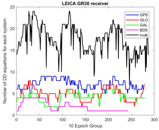
Figure 1.
Number of DD equations for each system in 10 epoch group windows.
The priori values of the variances for all four systems were set to 30 cm and 3 mm for code pseudorange and phase observations, respectively, and zero for all covariances in the first iteration. Note that the observables from different systems were considered completely uncorrelated. In the implementation of LS-VCE, the (co)variances of are estimated iteratively until the for two consecutive iterations are smaller than , while the time correlation is ignored. Although the satellite elevation dependence of the observations is taken into account, the inter-satellite/channel correlation was ignored. Moreover, the ambiguities are resolved by least squares ambiguity decorrelation adjustment (LAMBDA) [,].
For each GNSS system, the groupwise standard deviations calculated for C1, P2, L1, and L2 for the Trimble NETR9, SEPT POLARX5, and LEICA GR30 receivers, as well as their average values in 10 sequential epoch group windows, are shown in Figure 2, Figure 3 and Figure 4. The type of receiver used has an impact on the stochastic model determination. This is because each receiver uses its recovery technique to measure the code pseudorange and carrier phase measurements. The noise structure and, therefore, the stochastic model, can be affected by the general setup and antenna of the receiver [].
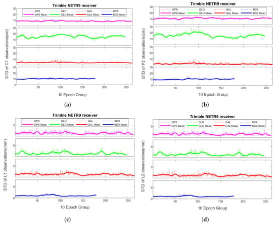
Figure 2.
Groupwise estimated standard deviations for each system (dashed line) with their average values in 10 epoch group windows (bold line) over a zero baseline with Trimble NETR9 receiver: (a,b) for the C1 and P2 in cm; (c,d) for the L1 and L2 in mm.
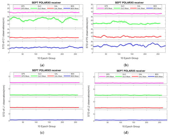
Figure 3.
Groupwise estimated standard deviations for each system (dashed line) with their average values in 10 epoch group windows (bold line) over a very short baseline with SEPT POLARX5 receiver: (a,b) for the C1 and P2 in cm; (c,d) for the L1 and L2 in mm.
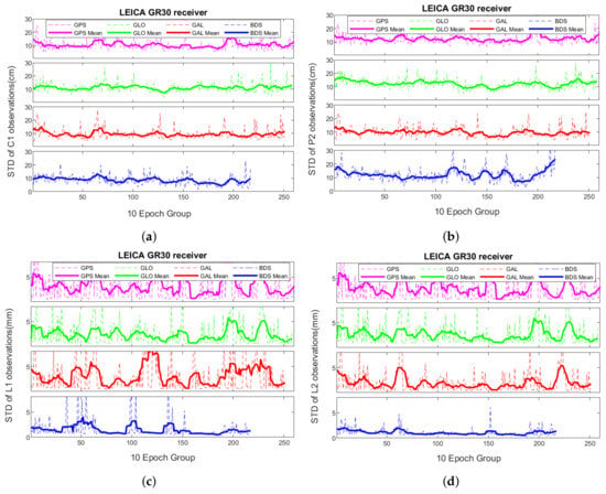
Figure 4.
Groupwise estimated standard deviations for each system (dashed line) with their average values in 10 epoch group windows (bold line) over a very short baseline with LEICA GR30 receiver: (a,b) for the C1 and P2 in cm; (c,d) for the L1 and L2 in mm.
For convenience, the mean values of the estimated standard deviations of four observation types for each system and their precision are presented in Table 2, Table 3 and Table 4. The results indicate that the estimated SDs of GPS observations are 85.62, 108.01, 1.47, and 1.58 mm for C1, P2, L1, and L2 for the Trimble NETR9 receiver. Similar to the GPS estimated variances, the BeiDou measurements have calculated SDs of 102.04, 100.62, 1.04, and 1.12 mm. Moreover, in the Trimble NETR9 receiver, the GLONASS measurements have the highest variances, with 152 mm, 156.66 mm, 1.43 mm, and 1.50 mm for C1, P2, L1, and L2, and the Galileo code observations have the lowest variances of all systems. In the SEPT POLARX5 receiver, GLONASS has the highest standard deviation for code observations, while the GALILEO has the lowest for the phase observations. The phase measurements of LEICA GR30 have the highest, and the SEPT POLARX5 have the lowest standard deviation. It’s worth noting that, as can be observed, the LEICA GR30 receiver’s observations are noisier, particularly for phase measurements. The final estimated variances, on the other hand, are not affected crucially.

Table 2.
Standard deviation of the phase and code observations and their precisions for each system, for Trimble NETR9 receiver over a zero baseline.

Table 3.
Standard deviation of the phase and code observations and their precision for each system for SEPT POLARX5 receiver over a very short baseline.

Table 4.
Standard deviation of the phase and code observations and their precision for each system for LEICA GR30 receiver over a very short baseline.
A similar scenario happens when it comes to the precision of the estimates. In most cases, the precision of the estimates for SEPT POLARX5 observations is the best, while for LEICA GR30, it is the worst. Moreover, for the Trimble NETR9 case, the precision of the estimates for Galileo code observations is the best at the sub-millimeter level, while the precision of the estimates for GLONASS code observations is the worst. The precision of phase variance estimates for all systems and all receivers, on the other hand, are at the micrometer level, which is likely too optimistic due to ignoring the temporal correlation, which has a colored noise effect instead of white noise.
The higher precision of L1 and C1 compared to L2 and P2 is due to the AS (Anti Spoofing) confrontation method of the receiver to measure the L2 and P2 in the phase tracking, and code tracking loops that lead to higher observations noise in these observation types [].
When considering the number of available satellites or the number of DD equations used to estimate the variances, we see that the number of equations and the variances are linked. Figure 5 depicted the number of equations and computed SD for LEICA GR30’s code and phase observations for GLONASS, respectively. It can be seen that when there are more visible satellites, the variances are lower.
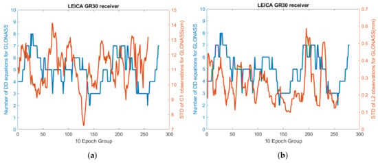
Figure 5.
Number of DD equations and the estimated SD for (a) C1 and (b) L2, for GLONASS in 10 epoch group windows.
Following the explanations of the LS-VCE method, the off-diagonal elements of the computed are the covariances between the observables of each system. As mentioned earlier, the observations from different systems were considered uncorrelated. Therefore, six correlations between C1 and P2, C1 and L1, C1 and L2, P2 and L1, P2 and L2, and L1 and L2 were estimated for each system. In addition, the correlation between the observation types was determined to make judgments. The precision of these estimations can also be obtained by applying the error propagation law to Equation (22). The reader is directed to [] for more detail.
The estimated values for different receivers are shown in Table 5, Table 6 and Table 7. Figure 6, Figure 7 and Figure 8, for example, show the groupwise estimated correlations between code observations for each system.

Table 5.
Covariances and correlation coefficient and their precision between the observation types for each system for the Trimble NETR9 receiver over a zero baseline.

Table 6.
Covariances and correlation coefficient and their precision between the observation types for each system for SEPT POLARX5 receiver over a very short baseline.

Table 7.
Covariances and correlation coefficient and their precision between the observation types for each system for LEICA GR30 receiver over a very short baseline.
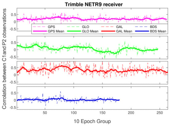
Figure 6.
Estimated correlation coefficients between the C1 and P2 observations (dashed line) with their average values in 10 epoch group windows (bold line) over a zero baseline.
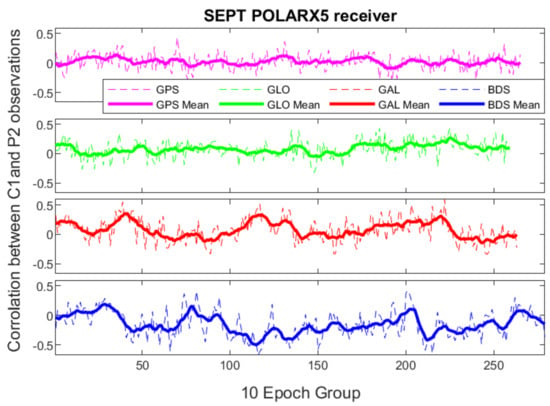
Figure 7.
Estimated correlation coefficients between the C1 and P2 observations (dashed line) with their average values in 10 epoch group windows (bold line) over a very short baseline.
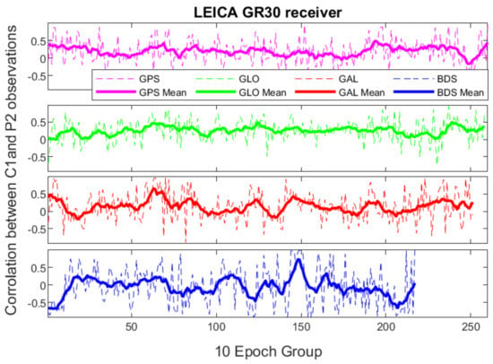
Figure 8.
Estimated correlation coefficients between the C1 and P2 observations (dashed line) with their average values in 10 epoch group windows (bold line) over a very short baseline.
The tables show that the correlations between two code and two phase observations are significant in most cases. The correlation values for the SEPT POLARX5 are the lowest, while Trimble NETR9 is the highest. The correlations between the phase observations are striking and for GPS is the highest with Trimble NETR9 and LEICA GR30. At the same time, BeiDou has the lowest correlation values in these two receivers among other systems.
One of the most critical steps in high-precision GNSS positioning, as previously indicated, is the IAR, which is influenced by a realistic estimate of the covariance matrix. The LAMBDA approach was employed in this paper as a integer least-squares ambiguity estimation method, resulting in the highest probability of a valid integer estimation. However, due to the risk of applying an incorrect integer solution, which could result in a large positioning error, the resolution of ambiguity includes not only integer estimation, but also validation. The integer bootstrapping ambiguity success rate (SR) is used as a critical metric to determine the reliability of integer ambiguity resolution. It displays the fraction or percentage of IAR that were successful. The bootstrapping method begins with the most precise float ambiguity becoming rounded. According to [], to enhance the bootstrapped success rate, one should work with decorrelated ambiguities rather than the original DD ambiguities, which have a significant correlation. Therefore, Z-transformation is used to transform the original ambiguities and the covariance matrix in the following form that and . So, the SR of integer bootstrapping can be estimated as follows []:
in which n represents the available ambiguities and the ambiguity derived through a conditioning on the previous I= consecutively rounded ambiguities, is denoted by the short-hand notation . Moreover, is the cumulative normal distribution, which is calculated according to the following manner:
If the precision of the float ambiguities improves, the bootstrapped success rate keeps increasing. As a result, integer bootstrapping will benefit from the GNSS model being strengthened. Therefore, the integer ambiguity success rate can be compared using two cases for single and multi-GNSS. In the first case, the nominal (co)variance in the stochastic model is used. In contrast, the estimated variances and covariances of the data set in the realistic stochastic model are introduced in the second case. Compared to a realistic stochastic model, a nominal stochastic model will reduce the precision of calculated parameters and result in a lower integer ambiguity success rate for all the systems. This paper is a follow-up to [], which demonstrates how using a more realistic stochastic model improves the IAR success rate for GPS observations. Table 8 shows the empirical success rate computed with nominal and realistic stochastic models and different receivers considering each system as well as multi-GNSS.

Table 8.
Estimated empirical success rate (SR) with Nominal and Realistic stochastic model in % (G:GPS, E:Galileo, R:GLONASS, C:BeiDou).
Finally, the estimated baseline component values are used as a criterion for evaluating the effect of adopting a realistic (co)variance matrix. Moreover, the estimated unknowns’ uncertainties (i.e., the baseline components deviation from zero) will be calculated by taking the square root of the diagonal components of the unknown covariance matrix approximated by . We estimated these values for two situations, one with a nominal and the other with a realistic stochastic model of the multi-GNSS observables. The difference between calculated baselines and real values, as well as their standard deviations, are shown in Table 9.

Table 9.
The difference between calculated baselines and real values and standard deviations with nominal and realistic stochastic model in multi-GNSS (mm).
5. Discussion
Estimating the variances and covariances of measurements in various receivers for the GPS, Galileo, GLONASS, and BeiDou systems yielded remarkable results based on the system and the receiver. As indicated in the figures and tables, the first noticeable issue was that the LEICA GR30 estimations were noisier. Even though this had practically no effect on the estimated parameters, it did significantly impact the precision of the estimated phase variances. Furthermore, among other receivers for phase observations, the SEPT POLARX5 is the most precise. The code measurement findings vary depending on the system and receiver. For example, we may claim that SEPT POLARX5 is the most excellent option for GPS code measurements, while Trimble NETR9 has the most precise code observations for Galileo. LEICA GR30 has the most precise observations for two other systems.
The covariances and correlations results revealed strong correlations between two phase and two code measurements, with the values for phase observations being significantly higher. This is because all GNSS satellites, as is well known, have at least two ranging codes. For instance, CA and P-codes are used in GPS. The first is for public use and is available to civilians. An unknown W-code encrypts the latter to generate the Y-code, which is only for military use. There are, however, several methods for tracking the P(Y) signal that does not require knowledge of the W-code. In other words, signal recovery techniques on the L1 frequency can not be used to measure the P-code or the L2 carrier in GPS receivers. With codeless or quasi-codeless techniques, GPS receivers can use L1 and CA-code information to perform measurements on the L2 carrier, and Y-code [,,]. The use of these techniques results in a correlation between code and phase observations [,]. Besides that, the correlation values also depend on the method used for the recovery techniques, which varies between different receivers. Furthermore, since the L2 phase tracking loop is not independent of L1 measurements, its SD values are higher. Table 5, Table 6 and Table 7 back up these claims. GLONASS and BeiDou are identical to GPS in that they both offer public and military positioning services. Unlike more military-oriented systems, however, the Galileo system is intended for civilian and commercial use []. Considering all the facts and results, it can be concluded that the precision of GNSS observations is receiver-dependent and system-dependent. That is where estimating a realistic stochastic model becomes vivid. However, in total, SEPT POLARX5 has the lowest correlation among others.
To evaluate the effect of applying a realistic stochastic model, the IAR success rate was estimated for two cases: the nominal and realistic stochastic model. When realistic variances and covariances are added into the process, it can be seen that the IAR success rate increases for each system as well as multi-GNSS data processing. The introduction of the realistic stochastic model can also lead to a realistic standard deviation of the baseline components. Compared to the basic stochastic model, the results of employing the realistic model indicated a reduction in these values. Although the changes are minor, given the baseline length, it can be claimed that using a realistic stochastic model in this experiment improves the results’ reliability. In the end, regardless of the system or receiver used, we can conclude that using a basic stochastic model leads to poorer precision of the predicted parameters. The results of LS-VCE for each receiver could be used in any other observation session. This procedure can also be thought of as the calibration of a specific receiver.
6. Conclusions
The observation weighting and the realistic stochastic model estimation is still a challenging problem in GNSS processing. To deal with this problem, the LS-VCE method was applied to real GNSS data sets collected by three multi-GNSS receivers (Trimble NETR9, SEPT POLARX5, and LEICA GR30) to estimate different variances and covariances for each GNSS observation type as well as the correlation between various observations. Considering these values and the observables’ satellite elevation dependence weighting, a realistic stochastic model for GNSS observables can be estimated and ultimately achieve the best linear unbiased estimators in high precision GNSS positioning. To repeat the LS-VCE scenario several times and reduce the processing time, the data were divided into 288 groups containing ten epochs of observations.
The results showed the estimated (co)variance values for Trimble NETR9 and SEPT POLARX5 are compatible. The Trimble NETR9 has the lowest and highest variances for Galileo and GLONASS code observations of all, respectively. On the SEPT POLARX5 receiver, GLONASS has the highest standard deviation for code observations, and GALILEO has the lowest for phase observations. The phase observations from the LEICA GR30 have the highest standard deviation, while those from the SEPT POLARX5 have the lowest. In most cases, the correlations between the phase observations are significantly larger than those between the code observations. Moreover, the correlation values for the SEPT POLARX5 are the lowest, while they are the highest for the Trimble NETR9. BeiDou has the lowest correlation values for Trimble NETR9 and LEICA GR30, among other systems.
In summary, the preliminary numerical results show that the stochastic model determination of the observables is highly dependent on the type of receiver used and the signal quality. This is because each receiver measures the code pseudorange and carrier phase measurements using its recovery method. Therefore, the overall design of the receiver and its antenna can affect the noise structure and hence the stochastic model. As a result, it is preferable to do the VCE before processing to obtain the BLUE of unknown parameters. This could be seen as a kind of calibration for the measurements of a specific GNSS receiver.
As previously mentioned, a realistic stochastic model affects the IAR success rate. The SR was compared in two cases, once with the nominal and once with the realistic (co)variance matrix used in the stochastic model. The results emphasized that using a more realistic stochastic model would increase IAR success rates in single and multi-GNSS cases. Affecting the IAR, using a realistic stochastic model based on LS-VCE, can shorten the TTF, which is a challenge for real-time positioning techniques.
Another criterion may be the impact of the realistic stochastic model on the estimated baseline components values and standard deviations, which are influenced by the observables’ weight matrix. In this way, the reported precision of the solution is realistic, neither too optimistic nor too pessimistic. The findings show that introducing the realistic stochastic model improves the baseline components’ standard deviation and accuracy and make them reliable. Considering all of the positive effects of utilizing a realistic stochastic model, we may evaluate the values of VCE for observations of each receiver and use the values in other upcoming processing.
Author Contributions
J.A. proposed the initial idea. F.M., J.A. and S.V. designed the algorithm and experiment. F.M. developed the software and wrote the manuscript. A.A.-S. All coauthors analyzed the results and reviewed and edited the manuscript. All authors have read and agreed to the published version of the manuscript.
Funding
This research was funded by Delft University of Technology.
Conflicts of Interest
The authors declare no conflict of interest.
References
- Wang, L.; Li, Z.; Zhao, J.; Zhou, K.; Wang, Z.; Yuan, H. Smart device-supported BDS/GNSS real-time kinematic positioning for sub-meter-level accuracy in urban location-based services. Sensors 2016, 16, 2201. [Google Scholar] [CrossRef] [PubMed] [Green Version]
- Wang, L.; Li, Z.; Yuan, H.; Zhao, J.; Zhou, K.; Yuan, C. Influence of the time-delay of correction for BDS and GPS combined real-time differential positioning. Electron. Lett. 2016, 52, 1063–1065. [Google Scholar] [CrossRef]
- Bosy, J.; Kaplon, J.; Rohm, W.; Sierny, J.; Hadas, T. Near real-time estimation of water vapour in the troposphere using ground GNSS and the meteorological data. In Annales Geophysicae; Copernicus GmbH: Göttingen, Germany, 2012; Volume 30, pp. 1379–1391. [Google Scholar]
- Hordyniec, P.; Bosy, J.; Rohm, W. Assessment of errors in Precipitable Water data derived from Global Navigation Satellite System observations. J. Atmos. Sol. Terr. Phys. 2015, 129, 69–77. [Google Scholar] [CrossRef]
- Chen, H.; Jiang, W.; Li, J. Multi-GNSS relative positioning with fixed inter-system ambiguity. Remote Sens. 2019, 11, 454. [Google Scholar] [CrossRef] [Green Version]
- Li, X.; Ge, M.; Dai, X.; Ren, X.; Fritsche, M.; Wickert, J.; Schuh, H. Accuracy and reliability of multi-GNSS real-time precise positioning: GPS, GLONASS, BeiDou, and Galileo. J. Geod. 2015, 89, 607–635. [Google Scholar] [CrossRef]
- Li, X.; Zhang, X.; Ren, X.; Fritsche, M.; Wickert, J.; Schuh, H. Precise positioning with current multi-constellation global navigation satellite systems: GPS, GLONASS, Galileo and BeiDou. Sci. Rep. 2015, 5, 8328. [Google Scholar] [CrossRef]
- Odolinski, R.; Teunissens, P.J.; Odijk, D. Combined GPS and BeiDou instantaneous RTK positioning. Navig. J. Inst. Navig. 2014, 61, 135–148. [Google Scholar] [CrossRef] [Green Version]
- Lau, L.; Tateshita, H.; Sato, K. Impact of multi-GNSS on positioning accuracy and multipath errors in high-precision single-epoch solutions–a case study in Ningbo China. J. Navig. 2015, 68, 999–1017. [Google Scholar] [CrossRef] [Green Version]
- Steigenberger, P.; Hugentobler, U.; Loyer, S.; Perosanz, F.; Prange, L.; Dach, R.; Uhlemann, M.; Gendt, G.; Montenbruck, O. Galileo orbit and clock quality of the IGS Multi-GNSS Experiment. Adv. Space Res. 2015, 55, 269–281. [Google Scholar] [CrossRef]
- Guo, J.; Xu, X.; Zhao, Q.; Liu, J. Precise orbit determination for quad-constellation satellites at Wuhan University: Strategy, result validation, and comparison. J. Geod. 2016, 90, 143–159. [Google Scholar] [CrossRef]
- Montenbruck, O.; Steigenberger, P.; Prange, L.; Deng, Z.; Zhao, Q.; Perosanz, F.; Romero, I.; Noll, C.; Stürze, A.; Weber, G.; et al. The Multi-GNSS Experiment (MGEX) of the International GNSS Service (IGS)–Achievements, prospects and challenges. Adv. Space Res. 2017, 59, 1671–1697. [Google Scholar] [CrossRef]
- Guo, F.; Li, X.; Zhang, X.; Wang, J. The contribution of Multi-GNSS Experiment (MGEX) to precise point positioning. Adv. Space Res. 2017, 59, 2714–2725. [Google Scholar] [CrossRef]
- Amiri-Simkooei, A.; Zangeneh-Nejad, F.; Asgari, J. Least-squares variance component estimation applied to GPS geometry-based observation model. J. Surv. Eng. 2013, 139, 176–187. [Google Scholar] [CrossRef]
- ICD. Global Navigation Satellite System GLONASS Interface Control Document, v5. 1.; Russian Institute of Space Device Engineering: Moscow, Russia, 2008. [Google Scholar]
- Leick, A.; Rapoport, L.; Tatarnikov, D. GPS Satellite Surveying; John Wiley & Sons: Hoboken, NJ, USA, 2015. [Google Scholar]
- Yang, Y.; Li, J.; Xu, J.; Tang, J.; Guo, H.; He, H. Contribution of the compass satellite navigation system to global PNT users. Chin. Sci. Bull. 2011, 56, 2813–2819. [Google Scholar] [CrossRef] [Green Version]
- Yang, Y.; Gao, W.; Guo, S.; Mao, Y.; Yang, Y. Introduction to BeiDou-3 navigation satellite system. Navig. J. Inst. Navig. 2019, 66, 7–18. [Google Scholar] [CrossRef] [Green Version]
- Amiri-Simkooei, A.R.; Jazaeri, S.; Zangeneh-Nejad, F.; Asgari, J. Role of stochastic model on GPS integer ambiguity resolution success rate. GPS Solut. 2016, 20, 51–61. [Google Scholar] [CrossRef]
- De Bakker, P.F.; Tiberius, C.C.; Van Der Marel, H.; van Bree, R.J. Short and zero baseline analysis of GPS L1 C/A, L5Q, GIOVE E1B, and E5aQ signals. GPS Solut. 2012, 16, 53–64. [Google Scholar] [CrossRef] [Green Version]
- Steigenberger, P.; Hugentobler, U.; Montenbruck, O. First demonstration of Galileo-only positioning. GPS World 2013, 24, 14–15. [Google Scholar]
- Montenbruck, O.; Hauschild, A.; Steigenberger, P.; Hugentobler, U.; Teunissen, P.; Nakamura, S. Initial assessment of the COMPASS/BeiDou-2 regional navigation satellite system. GPS Solut. 2013, 17, 211–222. [Google Scholar] [CrossRef]
- Gopaul, N.; Wang, J.G.; Scherzinger, B. Simplified algorithms of variance component estimation for static and kinematic GPS single point positioning. J. Glob. Position. Syst. 2009, 8, 43–52. [Google Scholar]
- Kazmierski, K.; Hadas, T.; Sośnica, K. Weighting of multi-GNSS observations in real-time precise point positioning. Remote Sens. 2018, 10, 84. [Google Scholar] [CrossRef] [Green Version]
- Han, J.; Huang, G.; Zhang, Q.; Tu, R.; Du, Y.; Wang, X. A new azimuth-dependent elevation weight (ADEW) model for real-time deformation monitoring in complex environment by multi-GNSS. Sensors 2018, 18, 2473. [Google Scholar] [CrossRef] [Green Version]
- Li, M.; Nie, W.; Xu, T.; Rovira-Garcia, A.; Fang, Z.; Xu, G. Helmert variance component estimation for multi-GNSS relative positioning. Sensors 2020, 20, 669. [Google Scholar] [CrossRef] [Green Version]
- Koch, K. Maximum likelihood estimate of variance components. Bull. Gæodésique 1986, 60, 329–338. [Google Scholar] [CrossRef]
- Koch, K.R. Parameter estimation in linear models. In Parameter Estimation and Hypothesis Testing in Linear Models; Springer: Berlin/Heidelberg, Germany, 1999; pp. 149–269. [Google Scholar]
- Teunissen, P.J.; Amiri-Simkooei, A. Least-squares variance component estimation. J. Geod. 2008, 82, 65–82. [Google Scholar] [CrossRef] [Green Version]
- Junhuan, P.; Yun, S.; Shuhui, L.; Honglei, Y. MINQUE of variance-covariance components in linear Gauss-Markov models. J. Surv. Eng. 2011, 137, 129–139. [Google Scholar] [CrossRef]
- Hofmann-Wellenhof, B.; Lichtenegger, H.; Wasle, E. GNSS–Global Navigation Satellite Systems: GPS, GLONASS, Galileo, and More; Springer Science & Business Media: Berlin/Heidelberg, Germany, 2007; pp. 101–102. [Google Scholar]
- Verhagen, S.; Odijk, D.; Boon, F.; Almansa, J.M.L. Reliable multi-carrier ambiguity resolution in the presence of multipath. In Proceedings of the 20th International Technical Meeting of the Satellite Division of The Institute of Navigation (ION GNSS 2007), Fort Worth, TX, USA, 25–28 September 2007; pp. 339–350. [Google Scholar]
- Teunissen, P.J.; Verhagen, S. The GNSS ambiguity ratio-test revisited: A better way of using it. Surv. Rev. 2009, 41, 138–151. [Google Scholar] [CrossRef]
- Zangeneh-Nejad, F.; Amiri-Simkooei, A.R.; Sharifi, M.A.; Asgari, J. On the realistic stochastic model of GPS observables: Implementation and Performance. Int. Arch. Photogramm. Remote Sens. Spat. Inf. Sci. 2015, 40, 755–761. [Google Scholar] [CrossRef] [Green Version]
- Teunissen, P.J. Quality Contzrol and GPS. In GPS for Geodesy; Springer: Berlin/Heidelberg, Germany, 1998; pp. 271–318. [Google Scholar]
- Teunissen, P.; Montenbruck, O. Springer Handbook of Global Navigation Satellite Systems; Springer: Berlin/Heidelberg, Germany, 2017. [Google Scholar]
- Teunissen, P. A new GLONASS FDMA model. GPS Solut. 2019, 23, 100. [Google Scholar] [CrossRef] [Green Version]
- Teunissen, P.; Khodabandeh, A. GLONASS ambiguity resolution. GPS Solut. 2019, 23, 1–11. [Google Scholar] [CrossRef] [Green Version]
- Zaminpardaz, S.; Teunissen, P.J.; Khodabandeh, A. GLONASS–only FDMA+ CDMA RTK: Performance and outlook. GPS Solut. 2021, 25, 1–12. [Google Scholar] [CrossRef]
- Brack, A. Rapid initialization for long baseline RTK positioning: Combined GPS+ Galileo+ BDS+ QZSS+ GLONASS with partial ambiguity resolution. In Proceedings of the 2020 European Navigation Conference (ENC), Dresden, Germany, 23–24 November 2020; pp. 1–9. [Google Scholar]
- Brack, A.; Männel, B.; Schuh, H. GLONASS FDMA data for RTK positioning: A five-system analysis. GPS Solut. 2021, 25, 1–13. [Google Scholar] [CrossRef]
- Amiri-Simkooei, A.; Teunissen, P.; Tiberius, C. Application of least-squares variance component estimation to GPS observables. J. Surv. Eng. 2009, 135, 149–160. [Google Scholar] [CrossRef] [Green Version]
- Teunissen, P.J.; Jonkman, N.; Tiberius, C. Weighting GPS dual frequency observations: Bearing the cross of cross-correlation. GPS Solut. 1998, 2, 28–37. [Google Scholar] [CrossRef] [Green Version]
- Bischoff, W.; Heck, B.; Howind, J.; Teusch, A. A procedure for estimating the variance function of linear models and for checking the appropriateness of estimated variances: A case study of GPS carrier-phase observations. J. Geod. 2006, 79, 694–704. [Google Scholar] [CrossRef]
- Amiri-Simkooei, A.R.; Tiberius, C.C.; Teunissen, P.J. Assessment of noise in GPS coordinate time series: Methodology and results. J. Geophys. Res. Solid Earth 2007, 112. [Google Scholar] [CrossRef] [Green Version]
- Jin, X.X.; de Jong, C.D. Relationship between satellite elevation and precision of GPS code observations. J. Navig. 1996, 49, 253–265. [Google Scholar]
- Wang, J.; Stewart, M.P.; Tsakiri, M. Stochastic modeling for static GPS baseline data processing. J. Surv. Eng. 1998, 124, 171–181. [Google Scholar] [CrossRef]
- Tiberius, C.; Jonkman, N.; Kenselaar, F. Innovation: The stochastics of GPS observables. GPS World 1999, 10, 49–54. [Google Scholar]
- Teunissen, P. The ionosphere-weighted GPS baseline precision in canonical form. J. Geod. 1998, 72, 107–111. [Google Scholar] [CrossRef]
- Bock, Y. Medium distance GPS measurements. In GPS for Geodesy; Springer: Berlin/Heidelberg, Germany, 1998; pp. 483–536. [Google Scholar]
- Teunissen, P. Towards a Least-Squares Framework for Adjusting and Testing of Both Functional and Stochastic Models; No. 26; Internal Research Memo, Geodetic Computing Centre: Delft, The Netherlands, 2004. [Google Scholar]
- Teunissen, P.J. Least-squares estimation of the integer GPS ambiguities. In Proceedings of the Invited Lecture, Section IV Theory and Methodology, IAG General Meeting, Beijing, China, 6 August 1993. [Google Scholar]
- Teunissen, P.; De Jonge, P.; Tiberius, C. The LAMBDA method for fast GPS surveying. In Proceedings of the International Symposium “GPS Technology Applications”, Bucharest, Romania, 26–29 September 1995. [Google Scholar]
- Teunissen, P.J. An optimality property of the integer least-squares estimator. J. Geod. 1999, 73, 587–593. [Google Scholar] [CrossRef]
- Teunissen, P.J. Success probability of integer GPS ambiguity rounding and bootstrapping. J. Geod. 1998, 72, 606–612. [Google Scholar] [CrossRef] [Green Version]
- Ashjaee, J.; Lorenz, R. Precise GPS surveying after Y-code. In Proceedings of the 5th International Technical Meeting of the Satellite Division of the Institute of Navigation (ION GPS 1992), Albuquerque, NM, USA, 16–18 September 1992; pp. 657–659. [Google Scholar]
- Seeber, G. Satellite Geodesy: Foundations, Methods, and Applications; Walter de Gruyter: Berlin, Germany, 2008; pp. 240–243. [Google Scholar]
- Amiri-Simkooei, A.; Tiberius, C. Assessing receiver noise using GPS short baseline time series. GPS Solut. 2007, 11, 21–35. [Google Scholar] [CrossRef] [Green Version]
- Chen, H.C.; Huang, Y.S.; Chiang, K.W.; Yang, M.; Rau, R.J. The performance comparison between GPs and BeiDou-2/compass: A perspective from Asia. J. Chin. Inst. Eng. 2009, 32, 679–689. [Google Scholar] [CrossRef]
Publisher’s Note: MDPI stays neutral with regard to jurisdictional claims in published maps and institutional affiliations. |
© 2021 by the authors. Licensee MDPI, Basel, Switzerland. This article is an open access article distributed under the terms and conditions of the Creative Commons Attribution (CC BY) license (https://creativecommons.org/licenses/by/4.0/).