
Internal Tides and Their Intraseasonal Variability on the Continental Slope Northeast of Taiwan Island Derived from Mooring Observations and Satellite Data

 , ,
, , 
Abstract
:1. Introduction
2. Data and Methods
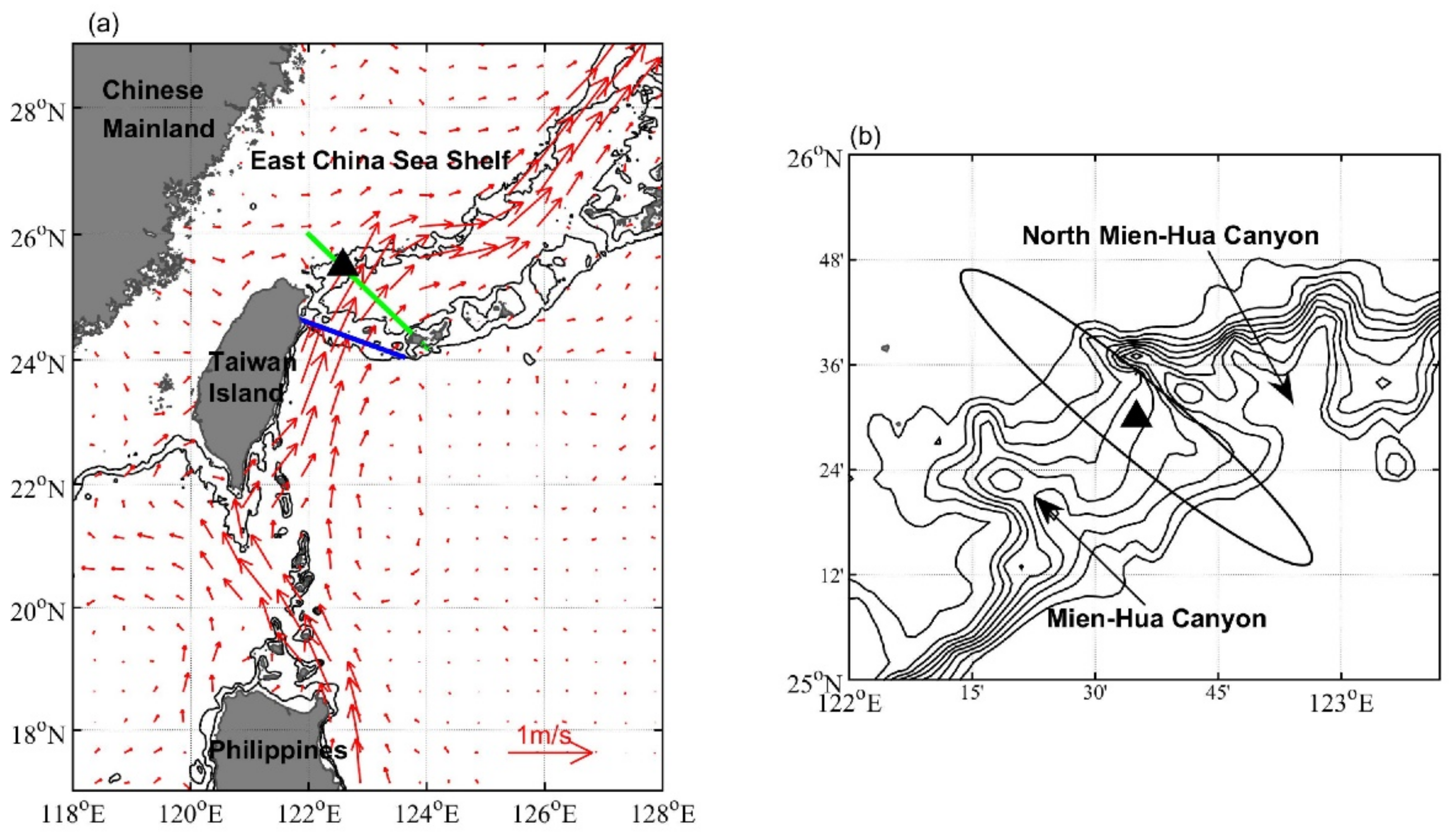
2.1. In Situ Velocities
2.2. Satellite Altimetry Data
2.3. Ocean Analysis Data
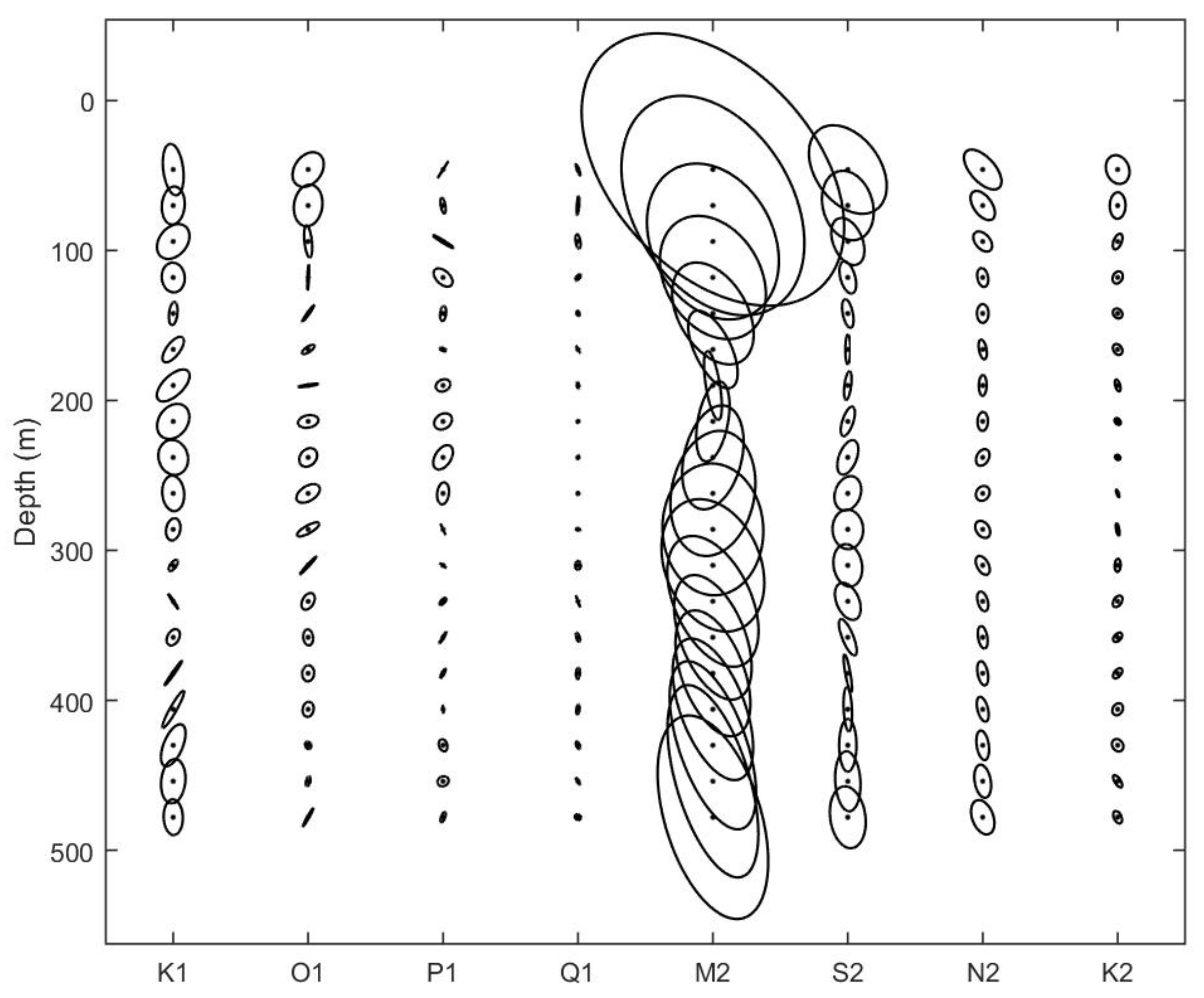
2.4. Tidal Harmonic Analyses
3. Results
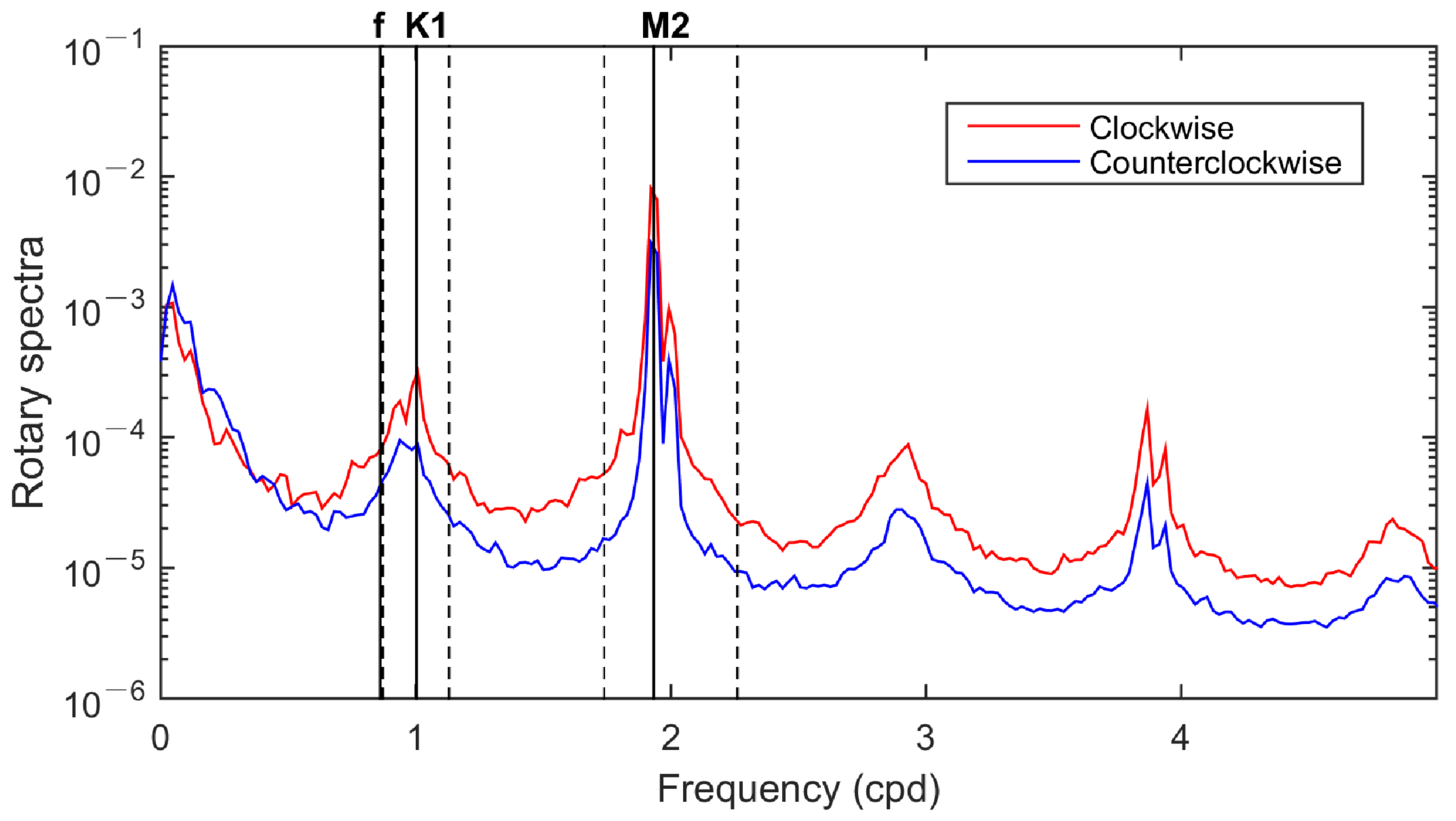
3.1. Barotropic Tides
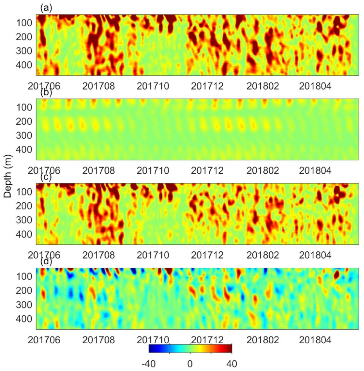
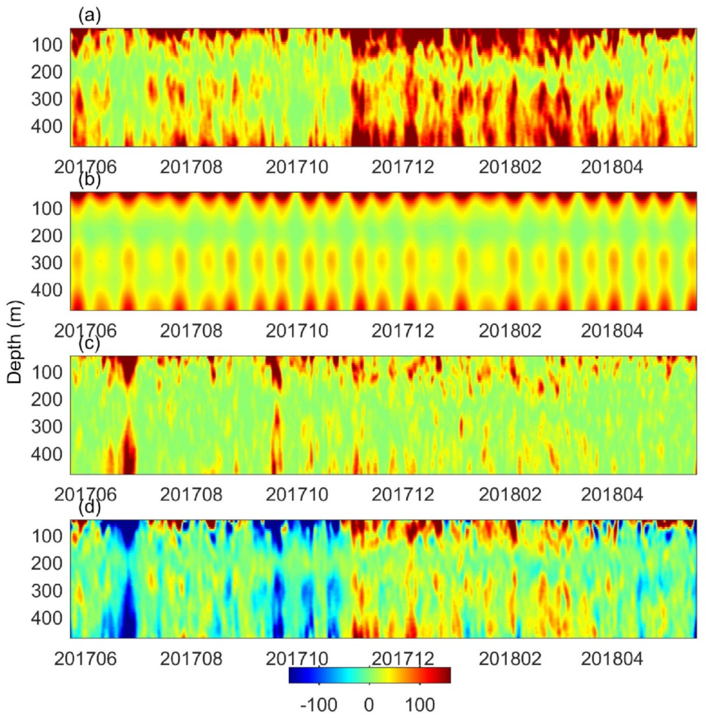
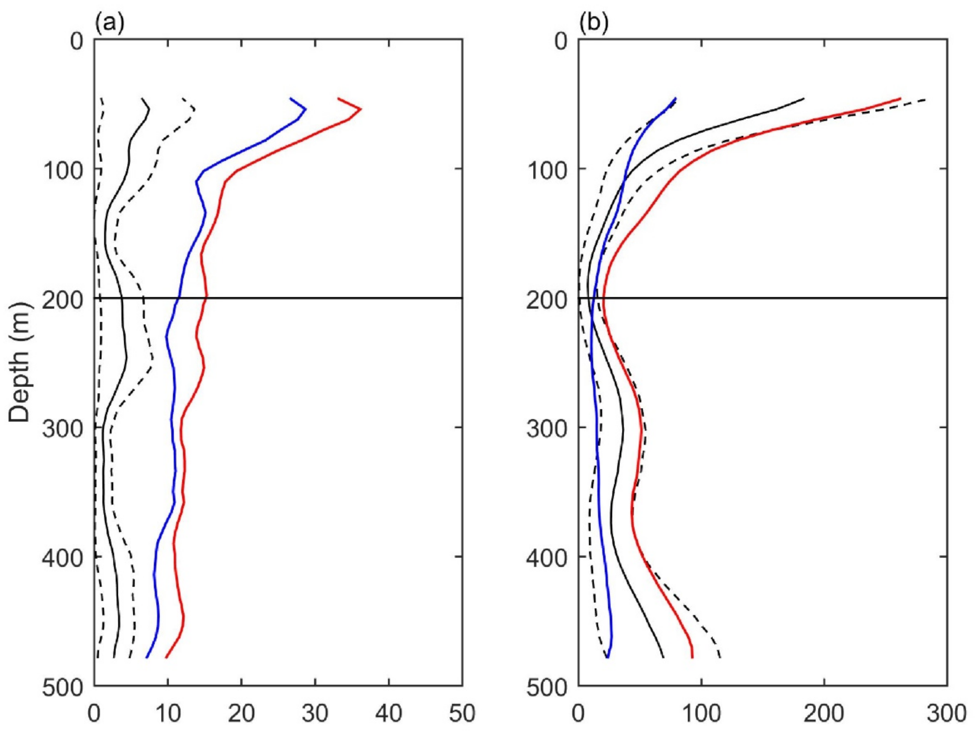
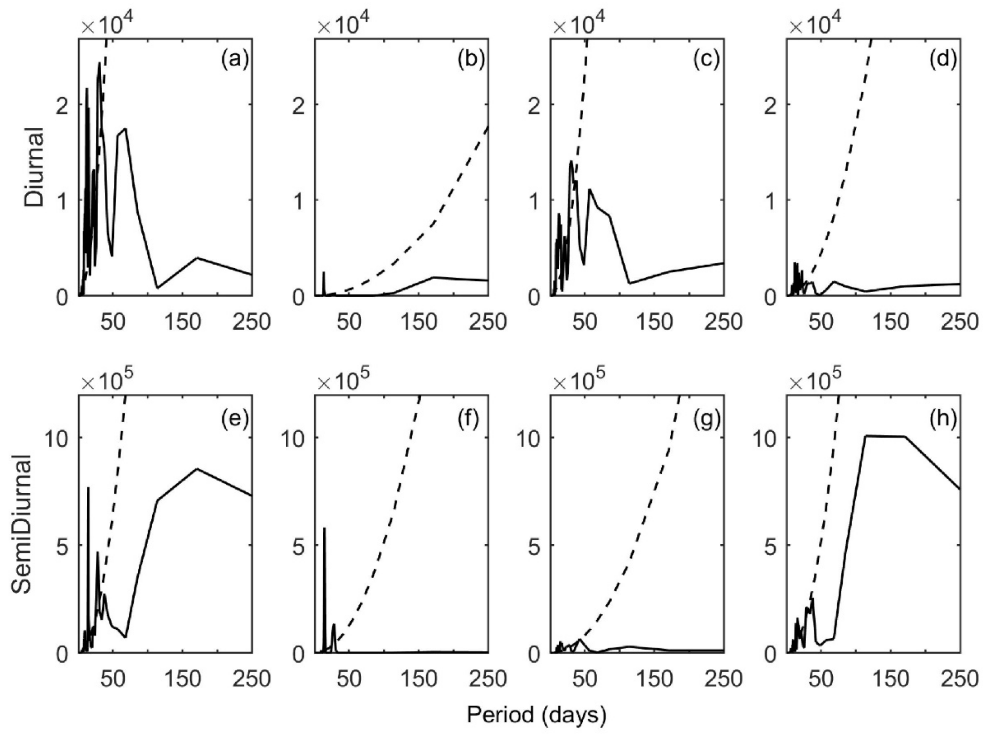
3.2. Internal Tides
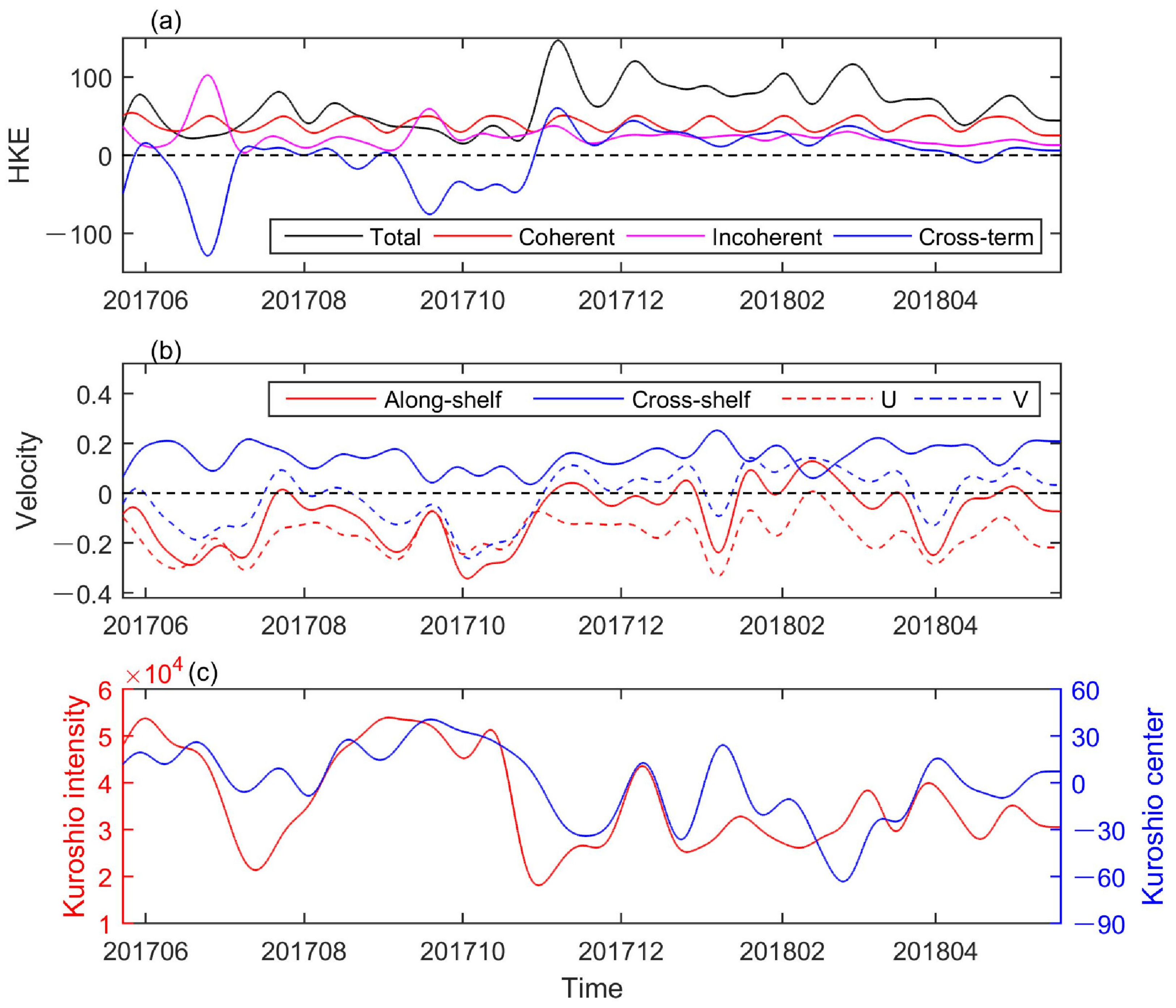
4. Discussion
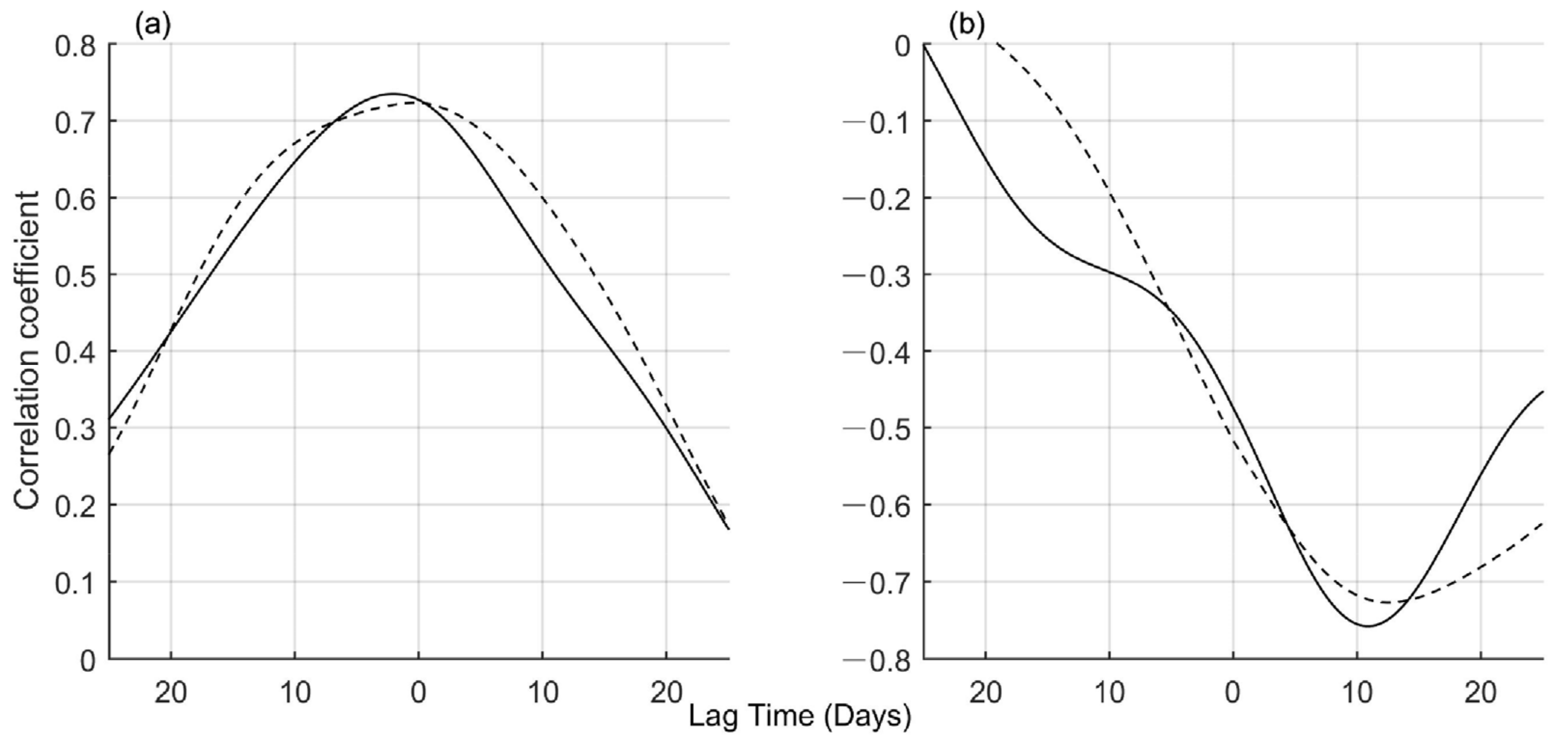
4.1. The Effect of Background Currents on Energy Propagation
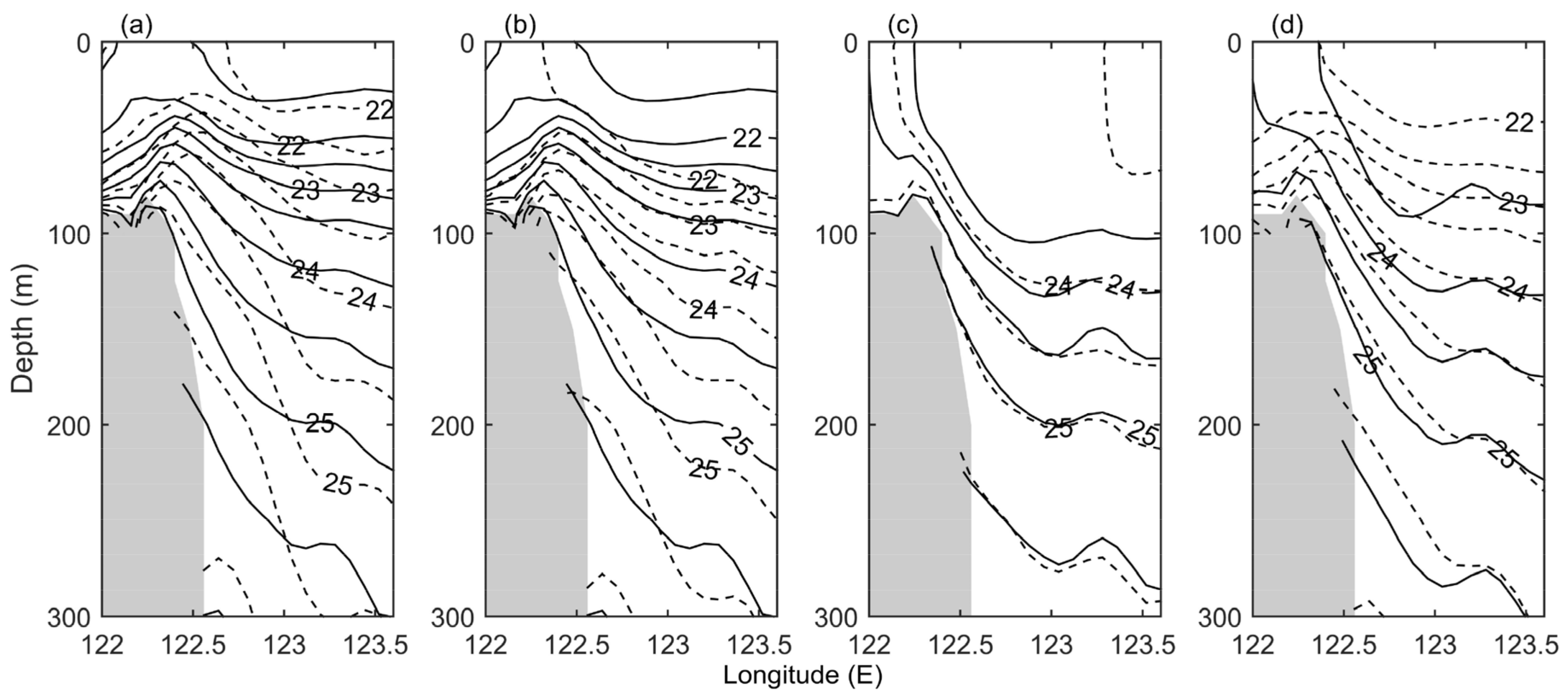
4.2. The Effect of Ocean Stratification on Energy Generation
4.3. The Effect of the Kuroshio Current and Mesoscale Eddies
5. Conclusions
Author Contributions
Funding
Institutional Review Board Statement
Informed Consent Statement
Data Availability Statement
Acknowledgments
Conflicts of Interest
References
- Baines, P. On internal tide generation models. Deep. Sea Res. Part A Oceanogr. Res. Pap. 1982, 29, 307–338. [Google Scholar] [CrossRef]
- Garrett, C.; Kunze, E. Internal Tide Generation in the Deep Ocean. Annu. Rev. Fluid Mech. 2007, 39, 57–87. [Google Scholar] [CrossRef]
- Chang, H.; Xu, Z.; Yin, B.; Hou, Y.; Liu, Y.; Li, D.; Wang, Y.; Cao, S.; Liu, A.K. Generation and Propagation of M 2 Internal Tides Modulated by the Kuroshio Northeast of Taiwan. J. Geophys. Res. Oceans 2019, 124, 2728–2749. [Google Scholar] [CrossRef]
- Wunsch, C.; Ferrari, R. Vertical mixing, energy, and the general circulation of the oceans. Annu. Rev. Fluid Mech. 2004, 36, 281–314. [Google Scholar] [CrossRef] [Green Version]
- Nagai, T.; Hasegawa, D.; Tanaka, T.; Nakamura, H.; Tsutsumi, E.; Inoue, R.; Yamashiro, T. First Evidence of Coherent Bands of Strong Turbulent Layers Associated with High-Wavenumber Internal-Wave Shear in the Upstream Kuroshio. Sci. Rep. 2017, 7, 14555. [Google Scholar] [CrossRef] [Green Version]
- Cimoli, L.; Caulfield, C.P.; Johnson, H.L.; Marshall, D.P.; Mashayek, A.; Garabato, A.N.; Vic, C. Sensitivity of Deep Ocean Mixing to Local Internal Tide Breaking and Mixing Efficiency. Geophys. Res. Lett. 2019, 43, 14622–14633. [Google Scholar] [CrossRef] [Green Version]
- Munk, W.; Wunsch, C. Abyssal recipes II: Energetics of tidal and wind mixing. Deep. Sea Res. Part I Oceanogr. Res. Pap. 1998, 45, 1977–2010. [Google Scholar] [CrossRef]
- Laurent, L.S.; Garrett, C. The Role of Internal Tides in Mixing the Deep Ocean. J. Phys. Oceanogr. 2002, 32, 2882–2899. [Google Scholar] [CrossRef] [Green Version]
- Williams, K.; Henyey, F.S.; Rouseff, D.; Reynolds, S.A.; Ewart, T. Internal wave effects on high-frequency acoustic propagation to horizontal arrays-experiment and implications to imaging. IEEE J. Ocean. Eng. 2001, 26, 102–112. [Google Scholar] [CrossRef]
- Wunsch, C. Internal tides in the ocean. Rev. Geophys. 1975, 13, 167–182. [Google Scholar] [CrossRef]
- Alford, M.H. Redistribution of energy available for ocean mixing by long-range propagation of internal waves. Nature 2003, 423, 159–162. [Google Scholar] [CrossRef] [PubMed]
- Alford, M.H.; Gregg, M.C.; Merrifield, M.A. Structure, Propagation, and Mixing of Energetic Baroclinic Tides in Mamala Bay, Oahu, Hawaii. J. Phys. Oceanogr. 2006, 36, 997–1018. [Google Scholar] [CrossRef]
- Zhao, Z.; Alford, M.H.; Girton, J.B.; Rainville, L.; Simmons, H.L. Global Observations of Open-Ocean Mode-1 M2 Internal Tides. J. Phys. Oceanogr. 2016, 46, 1657–1684. [Google Scholar] [CrossRef]
- Nakamura, T.; Awaji, T. Scattering of Internal Waves with Frequency Change over Rough Topography. J. Phys. Oceanogr. 2009, 39, 1574–1594. [Google Scholar] [CrossRef] [Green Version]
- Nikurashin, M.; Legg, S. A Mechanism for Local Dissipation of Internal Tides Generated at Rough Topography. J. Phys. Oceanogr. 2011, 41, 378–395. [Google Scholar] [CrossRef]
- Niwa, Y.; Hibiya, T. Numerical study of the spatial distribution of the M2internal tide in the Pacific Ocean. J. Geophys. Res. Space Phys. 2001, 106, 22441–22449. [Google Scholar] [CrossRef] [Green Version]
- Niwa, Y.; Hibiya, T. Three-dimensional numerical simulation of M2 internal tides in the East China Sea. J. Geophys. Res. Oceans 2004, 109. [Google Scholar] [CrossRef]
- Zhao, Z.; Klemas, V.; Zheng, Q.; Yan, X.-H. Remote sensing evidence for baroclinic tide origin of internal solitary waves in the northeastern South China Sea. Geophys. Res. Lett. 2004, 31, 06302. [Google Scholar] [CrossRef] [Green Version]
- Larsen, L.; Cannon, G.; Choi, B. East China Sea tide currents. Cont. Shelf Res. 1985, 4, 77–103. [Google Scholar] [CrossRef]
- Fang, G. Tide and tidal current charts for the marginal seas adjacent to China. Chin. J. Oceanol. Limnol. 1986, 4, 1–16. [Google Scholar]
- Li, L.; Jiang, W.; Li, P.; Yang, B. Vertical structure of the tidal currents on the continental shelf of the East China Sea. J. Ocean Univ. China 2012, 11, 347–353. [Google Scholar] [CrossRef]
- Guo, X.; Yanagi, T. Three-dimensional structure of tidal current in the East China Sea and the Yellow Sea. J. Oceanogr. 1998, 54, 651–668. [Google Scholar] [CrossRef]
- Da Silva, J.C.B.; New, A.L.; Srokosz, M.A.; Smyth, T. On the observability of internal tidal waves in remotely-sensed ocean colour data. Geophys. Res. Lett. 2002, 29, 10–11. [Google Scholar] [CrossRef]
- Kuroda, Y.; Mitsudera, H. Observation of internal tides in the East China Sea with an underwater sliding vehicle. J. Geophys. Res. Oceans 1995, 100, 10801. [Google Scholar] [CrossRef]
- Duda, T.F.; Newhall, A.E.; Gawarkiewicz, G.; Caruso, M.J.; Graber, H.C.; Yang, Y.J.; Jan, S. Significant internal waves and internal tides measured northeast of Taiwan. J. Mar. Res. 2013, 71, 47–81. [Google Scholar] [CrossRef] [Green Version]
- Lien, R.-C.; Sanford, T.B.; Jan, S.; Chang, M.-H.; Ma, B.B. Internal tides on the East China Sea Continental Slope. J. Mar. Res. 2013, 71, 151–185. [Google Scholar] [CrossRef]
- Liu, A.K.; Chang, Y.S.; Hsu, M.-K.; Liang, N.K. Evolution of nonlinear internal waves in the East and South China Seas. J. Geophys. Res. Oceans 1998, 103, 7995–8008. [Google Scholar] [CrossRef]
- Hsu, M.-K.; Liu, A.K.; Liu, C. A study of internal waves in the China Seas and Yellow Sea using SAR. Cont. Shelf Res. 2000, 20, 389–410. [Google Scholar] [CrossRef]
- Gerkema, T.; Lam, F.A.; Maas, L.R. Internal tides in the Bay of Biscay: Conversion rates and seasonal effects. Deep. Sea Res. Part II Top. Stud. Oceanogr. 2004, 51, 2995–3008. [Google Scholar] [CrossRef]
- Nash, J.D.; Kelly, S.M.; Shroyer, E.L.; Moum, J.N.; Duda, T. The Unpredictable Nature of Internal Tides on Continental Shelves. J. Phys. Oceanogr. 2012, 42, 1981–2000. [Google Scholar] [CrossRef] [Green Version]
- Pickering, A.; Alford, M.; Nash, J.; Rainville, L.; Buijsman, M.; Ko, D.S.; Lim, B. Structure and Variability of Internal Tides in Luzon Strait. J. Phys. Oceanogr. 2015, 45, 1574–1594. [Google Scholar] [CrossRef] [Green Version]
- Klymak, J.M.; Pinkel, R.; Rainville, L. Direct Breaking of the Internal Tide near Topography: Kaena Ridge, Hawaii. J. Phys. Oceanogr. 2008, 38, 380–399. [Google Scholar] [CrossRef]
- Cao, A.; Guo, Z.; Wang, S.; Chen, X.; Lv, X.; Song, J. Upper ocean shear in the northern South China Sea. J. Oceanogr. 2019, 75, 525–539. [Google Scholar] [CrossRef]
- Xu, Z.; Yin, B.; Hou, Y.; Xu, Y. Variability of internal tides and near-inertial waves on the continental slope of the northwestern South China Sea. J. Geophys. Res. Oceans 2013, 118, 197–211. [Google Scholar] [CrossRef]
- Du, T.; Tseng, Y.-H.; Yan, X.-H. Impacts of tidal currents and Kuroshio intrusion on the generation of nonlinear internal waves in Luzon Strait. J. Geophys. Res. Oceans 2008, 113, 08015. [Google Scholar] [CrossRef]
- Park, J.-H.; Farmer, D. Effects of Kuroshio intrusions on nonlinear internal waves in the South China Sea during winter. J. Geophys. Res. Oceans 2013, 118, 7081–7094. [Google Scholar] [CrossRef]
- Li, Q.; Wang, B.; Chen, X.; Chen, X.; Park, J. Variability of nonlinear internal waves in the South China Sea affected by the Kuroshio and mesoscale eddies. J. Geophys. Res. Oceans 2016, 121, 2098–2118. [Google Scholar] [CrossRef] [Green Version]
- Vlasenko, V.; Stashchuk, N.; Hutter, K. Baroclinic Tides; Cambridge University Press: Cambridge, UK, 2005; pp. 94–100. [Google Scholar]
- Jan, S.; Chern, C.-S.; Wang, J.; Chiou, M.-D. Generation and propagation of baroclinic tides modified by the Kuroshio in the Luzon Strait. J. Geophys. Res. Oceans 2012, 117, 02019. [Google Scholar] [CrossRef] [Green Version]
- Yuan, Y.; Zheng, Q.; Dai, D.; Hu, X.; Qiao, F.; Meng, J. Mechanism of internal waves in the Luzon Strait. J. Geophys. Res. 2006, 111, C11S17. [Google Scholar] [CrossRef] [Green Version]
- Xie, J.; He, Y.; Chen, Z.; Xu, J.; Cai, S. Simulations of internal solitary wave interactions with mesoscale eddies in the north-eastern South China Sea. J. Phys. Oceanogr. 2015, 45, 2959–2978. [Google Scholar] [CrossRef]
- Li, B.; Wei, Z.; Wang, X.; Fu, Y.; Fu, Q.; Li, J.; Lv, X. Variability of coherent and incoherent features of internal tides in the north South China Sea. Sci. Rep. 2020, 10, 12904. [Google Scholar] [CrossRef]
- Huang, X.; Zhang, Z.; Zhang, X.; Qian, H.; Zhao, W.; Tian, J. Impacts of a Mesoscale Eddy Pair on Internal Solitary Waves in the Northern South China Sea revealed by Mooring Array Observations. J. Phys. Oceanogr. 2017, 47, 1539–1554. [Google Scholar] [CrossRef]
- Ma, B.B.; Lien, R.-C.; Ko, D.S. The variability of internal tides in the Northern South China Sea. J. Oceanogr. 2013, 69, 619–630. [Google Scholar] [CrossRef]
- Zhang, D.; Lee, T.N.; Johns, W.E.; Liu, C.-T.; Zantopp, R. The Kuroshio East of Taiwan: Modes of Variability and Relationship to Interior Ocean Mesoscale Eddies. J. Phys. Oceanogr. 2001, 31, 1054–1074. [Google Scholar] [CrossRef]
- Vélez-Belchí, P.; Centurioni, L.R.; Lee, D.-K.; Jan, S.; Niiler, P.P. Eddy induced Kuroshio intrusions onto the continental shelf of the East China Sea. J. Mar. Res. 2013, 71, 83–107. [Google Scholar] [CrossRef]
- Yin, Y.; Lin, X.; He, R.; Hou, Y. Impact of mesoscale eddies on Kuroshio intrusion variability northeast of Taiwan. J. Geophys. Res. Oceans 2017, 122, 3021–3040. [Google Scholar] [CrossRef]
- Yin, Y.; Liu, Z.; Hu, P.; Hou, Y.; Lu, J.; He, Y. Impact of mesoscale eddies on the southwestward countercurrent northeast of Taiwan revealed by ADCP mooring observations. Cont. Shelf Res. 2020, 195, 104063. [Google Scholar] [CrossRef]
- Chelton, D.B.; Schlax, M.G.; Samelson, R.M. Global observations of nonlinear mesoscale eddies. Prog. Oceanogr. 2011, 91, 167–216. [Google Scholar] [CrossRef]
- Rio, M.H.; Guinehut, S.; Larnicol, G. New CNES-CLS09 global mean dynamic topography computed from the combination of GRACE data, altimetry, and in situ measurements. J. Geophys. Res. Oceans 2011, 116, 07018. [Google Scholar] [CrossRef]
- Chassignet, E.P.; Hurlburt, H.E.; Metzger, E.J.; Smedstad, O.M.; Cummings, J.A.; Halliwell, G.R.; Bleck, R.; Baraille, R.; Wallcraft, A.J.; Lozano, C.; et al. US GODAE: Global Ocean Prediction with the HYbrid Coordinate Ocean Model (HYCOM). Oceanography 2009, 22, 64–75. [Google Scholar] [CrossRef]
- Cummings, J.A.; Smedstad, O.M. Variational Data Assimilation for the Global Ocean. In Data Assimilation for Atmospheric, Oceanic and Hydrologic Applications; Park, S., Xu, L., Eds.; Springer: Berlin/Heidelberg, Germany, 2013; Volume 2, pp. 303–343. [Google Scholar]
- Chao, S.-Y. Circulation of the East China Sea, a numerical study. J. Oceanogr. 1990, 46, 273–295. [Google Scholar] [CrossRef]
- Oey, L.-Y.; Hsin, Y.-C.; Wu, C.-R. Why does the Kuroshio northeast of Taiwan shift shelfward in winter? Ocean Dyn. 2010, 60, 413–426. [Google Scholar] [CrossRef]
- James, C.; Wimbush, M.; Ichikawa, H. Kuroshio Meanders in the East China Sea. J. Phys. Oceanogr. 1999, 29, 259–272. [Google Scholar] [CrossRef]
- Zhao, X.; Hou, Y.; Liu, Z.; Zhuang, Z.; Wang, K. Seasonal Variability of Internal Tides Northeast of Taiwan. J. Ocean Univ. China 2020, 19, 740–746. [Google Scholar] [CrossRef]
- Johns, W.E.; Lee, T.N.; Zhang, D.X.; Zantopp, R.; Liu, C.T.; Yang, Y. The Kuroshio east of Taiwan: Moored transport observations from the WOCE PCM-1 array. J. Phys. Oceanogr. 2001, 31, 1031–1053. [Google Scholar] [CrossRef] [Green Version]
- Rainville, L.; Pinkel, R. Observations of Energetic High-Wavenumber Internal Waves in the Kuroshio. J. Phys. Oceanogr. 2004, 34, 1495–1505. [Google Scholar] [CrossRef]
- He, Y.; Hu, P.; Yin, Y.; Liu, Z.; Liu, Y.; Hou, Y.; Zhang, Y. Vertical Migration of the Along-Slope Counter-Flow and Its Relation with the Kuroshio Intrusion off Northeastern Taiwan. Remote Sens. 2019, 11, 2624. [Google Scholar] [CrossRef] [Green Version]
- Ji, C.; Zhang, Y.; Cheng, Q.; Li, Y.; Jiang, T.; Liang, X.S. Analyzing the variation of the precipitation of coastal areas of eastern China and its association with sea surface temperature (SST) of other seas. Atmos. Res. 2019, 219, 114–122. [Google Scholar] [CrossRef]
- Ji, C.; Zhang, Y.; Cheng, Q.; Tsou, J.; Jiang, T.; Liang, X.S. Evaluating the impact of sea surface temperature (SST) on spatial distribution of chlorophyll-a concentration in the East China Sea. Int. J. Appl. Earth Obs. Geoinf. 2018, 68, 252–261. [Google Scholar] [CrossRef]
- Zhang, Y.; Huang, Z.; Fu, D.; Tsou, J.; Jiang, T.; Liang, X.; Lu, X. Monitoring of chlorophyll-a and sea surface silicate concen-trations in the south part of Cheju island in the East China Sea using MODIS data. Int. J. Appl. Earth Obs. Geoinf. 2018, 67, 173–178. [Google Scholar] [CrossRef]
- Hsin, Y.-C.; Qiu, B.; Chiang, T.-L.; Wu, C.-R. Seasonal to interannual variations in the intensity and central position of the surface Kuroshio east of Taiwan. J. Geophys. Res. Oceans 2013, 118, 4305–4316. [Google Scholar] [CrossRef]
- Ichikawa, K.; Tokeshi, R.; Kashima, M.; Sato, K.; Matsuoka, T.; Kojima, S.; Fujii, S. Kuroshio variations in the upstream region as seen by HF radar and satellite altimetry data. Int. J. Remote Sens. 2008, 29, 6417–6426. [Google Scholar] [CrossRef]
- Tang, T.; Tai, J.-H.; Yang, Y.-J. The flow pattern north of Taiwan and the migration of the Kuroshio. Cont. Shelf Res. 2000, 20, 349–371. [Google Scholar] [CrossRef]
- Liu, C.; Wang, F.; Chen, X.; Von Storch, J.-S. Interannual variability of the Kuroshio onshore intrusion along the East China Sea shelf break: Effect of the Kuroshio volume transport. J. Geophys. Res. Oceans 2014, 119, 6190–6209. [Google Scholar] [CrossRef] [Green Version]
- Isobe, A. Recent advances in ocean-circulation research on the Yellow Sea and East China Sea shelves. J. Oceanogr. 2008, 64, 569–584. [Google Scholar] [CrossRef]


| Constituents | K1 | O1 | P1 | Q1 | M2 | S2 | N2 | K2 |
|---|---|---|---|---|---|---|---|---|
| Amplitude (cm s−1) | 1.86 | 1.27 | 0.44 | 0.38 | 24.12 | 7.47 | 4.11 | 1.78 |
| Phase (°) | 115 | 75 | 135 | 50 | 185 | 226 | 154 | 230 |
| Inclination (°) | 133 | 125 | 129 | 124 | 140 | 138 | 141 | 146 |
| Zonal Velocity | Meridional Velocity | Along-Shelf Velocity | Cross-Shelf Velocity | Kuroshio Intensity | Kuroshio Center | |
|---|---|---|---|---|---|---|
| HKE | 0.39 | 0.73 | 0.69 | 0.23 | −0.76 (10.88 d) | −0.68 (6.25 d) |
| HKEcr | 0.26 | 0.72 | 0.65 | 0.40 | −0.73 (12.58 d) | −0.67 (2.67 d) |
Publisher’s Note: MDPI stays neutral with regard to jurisdictional claims in published maps and institutional affiliations. |
© 2021 by the authors. Licensee MDPI, Basel, Switzerland. This article is an open access article distributed under the terms and conditions of the Creative Commons Attribution (CC BY) license (https://creativecommons.org/licenses/by/4.0/).
Share and Cite
Yin, Y.; Liu, Z.; Zhang, Y.; Chu, Q.; Liu, X.; Hou, Y.; Zhao, X. Internal Tides and Their Intraseasonal Variability on the Continental Slope Northeast of Taiwan Island Derived from Mooring Observations and Satellite Data. Remote Sens. 2022, 14, 59. https://doi.org/10.3390/rs14010059
Yin Y, Liu Z, Zhang Y, Chu Q, Liu X, Hou Y, Zhao X. Internal Tides and Their Intraseasonal Variability on the Continental Slope Northeast of Taiwan Island Derived from Mooring Observations and Satellite Data. Remote Sensing. 2022; 14(1):59. https://doi.org/10.3390/rs14010059
Chicago/Turabian StyleYin, Yuqi, Ze Liu, Yuanzhi Zhang, Qinqin Chu, Xihui Liu, Yijun Hou, and Xinhua Zhao. 2022. "Internal Tides and Their Intraseasonal Variability on the Continental Slope Northeast of Taiwan Island Derived from Mooring Observations and Satellite Data" Remote Sensing 14, no. 1: 59. https://doi.org/10.3390/rs14010059
APA StyleYin, Y., Liu, Z., Zhang, Y., Chu, Q., Liu, X., Hou, Y., & Zhao, X. (2022). Internal Tides and Their Intraseasonal Variability on the Continental Slope Northeast of Taiwan Island Derived from Mooring Observations and Satellite Data. Remote Sensing, 14(1), 59. https://doi.org/10.3390/rs14010059