Few-Shot Learning for Post-Earthquake Urban Damage Detection

Abstract

Among natural disasters, earthquakes are recorded to have the highest rates of human loss in the past 20 years. Their unexpected nature has severe consequences on both human lives and material infrastructure, demanding urgent action to be taken. For effective emergency relief, it is necessary to gain awareness about the level of damage in the affected areas. The use of remotely sensed imagery is popular in damage assessment applications; however, it requires a considerable amount of labeled data, which are not always easy to obtain. Taking into consideration the recent developments in the fields of Machine Learning and Computer Vision, this study investigates and employs several Few-Shot Learning (FSL) strategies in order to address data insufficiency and imbalance in post-earthquake urban damage classification. While small datasets have been tested against binary classification problems, which usually divide the urban structures into collapsed and non-collapsed, the potential of limited training data in multi-class classification has not been fully explored. To tackle this gap, four models were created, following different data balancing methods, namely cost-sensitive learning, oversampling, undersampling and Prototypical Networks. After a quantitative comparison among them, the best performing model was found to be the one based on Prototypical Networks, and it was used for the creation of damage assessment maps. The contribution of this work is twofold: we show that oversampling is the most suitable data balancing method for training Deep Convolutional Neural Networks (CNN) when compared to cost-sensitive learning and undersampling, and we demonstrate the appropriateness of Prototypical Networks in the damage classification context.

1. Introduction

Earthquakes are events of episodic nature, which can have a grave impact on human life and cause immense property loss. The Centre for Research on the Epidemiology of Disasters (CRED) and UN Office for Disaster Risk Reduction (UNDRR) [1] report on the cost of disasters for the period 2000–2019 declared earthquakes as the deadliest type of disaster for the first two decades of the 21st century, and highlight their potential for massive damage to infrastructure. Given that earthquakes are unpredictable, both in terms of time and magnitude, responding appropriately after the event is often critical to minimize the number of casualties. The success of emergency response operations relies on efficient organizational management and rapid reaction. A mandatory precondition to fulfill these requirements is to gain Situational Awareness: to know what has happened, when and where. The suitability of Machine Learning (ML) [2] techniques in different phases of disaster mitigation has been exhibited in recent studies. Harirchian et al. [3] assess the seismic vulnerability given a set of quantifiable parameters. The regional seismicity can also be monitored using ML if the automatically captured ambient noise data are subjected to Convolutional Neural Network (CNN)-based classifiers in order to detect earthquake events [4]. In the post-disaster phase, ML approaches have been employed to locate and measure post-earthquake urban damage, confirming the relevance of this field for such kinds of applications [5,6,7,8,9,10,11,12,13,14,15]. Pre-event seismic vulnerability assessment, earthquake magnitude evaluation and post-event damage detection are complementary aspects of disaster mitigation and, if combined, can provide valuable insights to local stakeholders for traffic network disruption modeling, restoration planning and cost estimation [16].

To identify the locations that require immediate relief, remotely sensed data are commonly used because they can provide an overview of a large region at once, and acquiring them does not pose the same risks as collecting ground-truth data [11]. In the context of emergency mapping, remotely sensed data usually refer to imagery acquired via satellite, Unmanned Aerial Vehicles (UAVs) or other aerial platforms [17]. As the availability of this kind of data and the processing power of modern computational systems have been constantly increasing, the possibility of automating the identification and assessment of post-disaster damage is also being explored [18]. For this reason, computer vision methods are employed, aiming to minimize the time overhead and the error that is introduced by the human factor [9]. Recent studies have demonstrated that ML algorithms outperform traditional Remote Sensing techniques in image classification tasks [19]. One of the main obstacles to overcome in the identification of earthquake damage is the small number of training samples [6]. The methodology that we follow in this study is based on Few-Shot Learning (FSL), which is a type of ML method, where the available data for the target classification task contains only a limited number of examples with supervised information [20]. Since destructive seismic events rarely happen but reacting quickly in such cases is crucial, FSL is competent when it comes to extracting knowledge from a narrow amount of data, and thus, the required effort for data gathering is also reduced. However, an FSL problem is not easy to solve. The lack of data requires a different approach than other ML problems, which rely on having a plethora of samples to train the model. The suggested solutions may vary in terms of algorithm, model parameters and data handling [20].

Related research papers that have incorporated FSL for locating ravaged buildings focus on binary classification rather than further dividing buildings into different wreckage levels [5,6,8,10,12]. Multi-class categorization, though, can emphasize or even create class imbalances within the data. The present study seeks to fill this gap by leveraging FSL to tackle data deficiency for certain classes in a multi-class problem. There are several means of dealing with data deficiency [20,21] and imbalance [22]. Applications that track disaster-related damage with ML can benefit from the existence of pre-event data, but on some occasions, this kind of data may be impossible to acquire. For this reason, we examine how efficient can a model be that is based only on post-event data. The purpose of this study is to implement and evaluate the effect of different FSL approaches on an imbalanced dataset. More precisely, we explore how can the supervised classification of a highly imbalanced dataset be elaborated, to what extent are the representatives of the majority and minority classes successfully detected and how indicative is the map overlay of the predictions for the severity of damage suffered by a geographic region.

The rest of the document is organized as follows. Section 2 reviews related studies, considers the applied research approaches and analyzes the theoretical background that is necessary to follow the present study. Section 3 presents the data and the methodological workflow. Section 4 explains the results of the study and is followed by Section 5, which discusses the results and proposes future research directions. Finally, Section 6 concludes the work.

2. Related Work

2.1. Remote Sensing in Emergency Mapping

Boccardo and Tonolo [17] have created a systematic review concerning the role of Remote Sensing in post-disaster damage mapping. Based on their paper, optical imagery is favored over Synthetic Aperture Radar (SAR) imagery for damage estimation, as it permits finer spatial resolution and is semantically richer, which is crucial in operational conditions. Nevertheless, Ge et al. [23] emphasize on the key role of SAR data when the atmospheric conditions do not allow optical sensors to capture imagery of quality. The existence of pre-event data is mentioned to add up to the quality of collapsed building detection [17]. According to Cooner et al. [5], ML algorithms gain popularity in damage assessment applications, due to outperforming traditional methods for change detection and image classification and due to being capable of dealing with non-linear datasets. The authors compared Random Forest (RF), Artificial Neural Network (ANN) and Radial Basis Function Neural Network (RBFNN) algorithms on panchromatic and multispectral VHR imagery obtained by the satellites WordView1 and QuickBird2. The study concluded that ANN demonstrates the lowest Error of Omission and the shortest training time, while the model could be produced with only panchromatic imagery.

Li et al. [24] performed an extensive survey about object detection in optical Remote Sensing images. As stated in the paper, Deep Learning algorithms are currently the predominant approach for visual recognition tasks, including object detection related to the fields of Computer Vision and Earth Observation. Although in Computer Vision, the employed methods can be region proposal-based or regression-based, Earth Observation applications favor the first approach [24]. The study also proposed a new benchmark dataset, characterized by low inter-class and high intra-class variability and tested it with different combinations of backbone and object prediction architectures, stating that deeper backbone networks demonstrate a higher Overall Accuracy.

Different incident types affect urban structures differently [11]. However, we assume that earthquake and wind-induced damages are comparable because they impact the structural materials in a similar way, causing lateral damage to the constructions [25,26]. For this reason, hurricane-related studies are also included in the literature review.

2.2. Deep Learning for Urban Damage Assessment

Anniballe et al. [8] analyzed multispectral and panchromatic, bi-temporal images of a small geographic region with the Bayesian Maximum A Posteriori (MAP) criterion and the Support Vector Machine (SVM). The study followed a five-level scale for damage assessment, but the results reported are grouped in heavy damaged buildings (damage grade = 5) and less damaged buildings (damage grade < 5). SVM demonstrated better performance than the MAP classifier for this study case.

Ji et al. [6] applied a CNN architecture called SqueezeNet on single-temporal post-earthquake VHR QuickBird imagery. The study divided the buildings in the city of Port-au-Prince after the Haiti 2010 incident into two categories: collapsed and non-collapsed. As the non-collapsed buildings outnumbered the completely destroyed ones, the researchers used three different data balancing methods, namely random oversampling, random undersampling and cost-sensitive, to improve the accuracy.

Ji et al. [12] have shown the potential of pre-trained CNN (VGGNet) models for post-earthquake damage identification. Two models were compared, one trained from scratch and one pre-trained on the benchmark dataset ImageNet [27], with the accuracy results greatly favoring the latter. Both models were fed with labeled bi-temporal VHR imagery and were responsible for binary classification of the buildings: collapsed and non-collapsed. The study also points out the risk of overfitting when the data are limited and makes use of data augmentation to figuratively expand the dataset. Li et al. [10] have also derived similar results when comparing a fine-tuned pre-trained model of Single-Shot Multibox Detector (SSD) with one trained from scratch for identifying post-hurricane structural damage. In contrast with Ji et al. [12], this study used single post-event aerial imagery for classifying the damage at two different levels: damaged and debris.

Xu et al. [9] performed a comparative study of four different models using the Haiti 2010 dataset. Three of the models were built using both pre and post-disaster-labeled images, and one was built using single post-earthquake data. The study tested the generalization ability of the best-performing model and found it more competent as the number of earthquake incidents that are included in the training increases. The reason is the low variability that characterizes each individual incident dataset, a fact that can lead to overfitting [9].

The need for a common framework for building damage assessment after different kinds of natural disasters (earthquakes, floods, hurricanes, wildfires, volcanic eruptions, etc.) has been highlighted by Gupta et al. [11]. The study discusses the need for having a benchmark dataset that is compliant with the requirements of ML algorithms taking into account the rarity of occurrences of a large-scale natural disaster and hence the relevant data shortage. The study’s main contribution is a dataset that consists of bi-temporal VHR labeled satellite imagery from various disaster incidents. The produced xBD dataset has already been used to train and evaluate ML classifiers for damage in the works of other researchers [14,15,28]. Valentijn et al. [14] have trained Inception-v3-based CNN models, trying to simulate operational conditions, while Bai et al. [15] developed a combination of a semi-Siamese network with a pyramid-pooling module. The aforementioned studies follow an end-to-end approach for damage localization and classification, meaning that the building extraction is part of the ML pipeline. Touzani and Granderson [29] have outlined the necessity for creating accurate Deep Learning models that recognize urban structures and propose a method for automatic extraction of buildings in openly available datasets based on semantic segmentation in order to create a unified training dataset with high variability that contains them all.

The transferability of pre-trained CNN models to new disaster occasions was also examined by Vetrivel et al. [7]. The study integrated 3D point cloud data on top of vertical and oblique aerial photography. Among the models that were employed, the authors recommend the use of a pre-trained CNN as a feature extractor with no further weight tuning because it can achieve Overall Accuracy of the same levels without being as costly in terms of data and computation. However, the inclusion of site-specific samples can positively impact the model’s performance [7].

Li et al. [13], taking into consideration the amount of time that labeled data needs to be produced, have employed an unsupervised domain adaptation model based on unlabeled post-hurricane imagery. The model, despite its complexity, as it consists of several Generative Adversarial Networks (GANs), a classifier and a self-attention module, was evaluated by the authors as successful with regards to the transfer learning tasks that were assigned to it.

2.3. Comparative Analysis

The aforementioned studies concern related applications, where post-disaster urban damage is tracked with ML. The approaches vary greatly with regards to the methods employed. The input imagery and the number of the predicted classes are parameters that affect the design of the learning pipeline. The input imagery and the number of the predicted classes are parameters that affect the design of the learning pipeline.

Table 1. Data parameters that affect the architecture design. Dataset size refers to building instances.

Study	Data Source	Dataset Size	ML Approach	Classes
Cooner et al. [5]	Satellite—Bi-temporal	897	RF, ANN, RBFNN	2
Ji et al. [6]	Satellite—Single post-event	3928	SqueezeNet, data balancing	2
Vetrivel et al. [7]	Airborne—Bi-temporal	12,544	CNN, pre-trained CNN	2
Anniballe et al. [8]	Satellite—Bi-temporal	1667	SVM, MAP	2
Xu et al. [9]	Satellite—Single post-event	75,468	AlexNet	2
Li et al. [10]	Airborne—Single post-event	757	SSD, data augmentation	2
Gupta et al. [11]	Satellite—Single post-event	632,228	Shallow CNN and ResNet50	4
Ji et al. [12]	Satellite—Bi-temporal	1789	VGGNet, pre-trained VGGNet, data augmentation	2
Li et al. [13]	Airborne—Single post-event	34,000	GANs and classifier and self-attention module	3
Valentijn et al. [14]	Satellite—Bi-temporal	850,736	Inception-v3 CNN	4
Bai et al. [15]	Satellite—Bi-temporal	>850,000	Pyramid Pooling Module and Semi-Siamese Network	4

summarizes the parameters that were encountered in the literature and were evaluated as fundamental for the creation of the predictive model, namely data source (satellite/airborne, single/bi-temporal), dataset size, ML approach and number of output classes.

The most common incident among earthquake-related studies is the Haiti 2010 earthquake and has often been the unique data source of the analysis [5,6,12]. Given that the models built on very specific data have a poor generalization ability [9], newer studies are incorporating more earthquake incidents [7,9] or do not distinguish between the damage cause, especially the ones utilizing the dedicated xBD dataset [11,14,15]. The preferred imagery type in the relevant ML applications is of VHR, acquired either by satellite (usually WorldView and QuickBird) or by aerial platforms. Additional data sources, such as 3D point cloud features [7], can be used collaterally, but the basis for the learning process remains optical imagery, which is also meaningful to human vision.

To overcome a possible data shortage and accelerate the creation of a competent predictive model, a plethora of approaches have been put to use. Pre-trained models can transfer knowledge and save time and computational resources [7,12]. Data augmentation is necessary for small datasets [10] and data balancing for non-linear datasets [6,15]. Unsupervised classification is also gaining popularity [24], as it minimizes the effort for labeling the training data. All the aforementioned strategies are possible solutions to an FSL problem. FSL has already been introduced as a means of dealing with emergency situations [30,31,32]. However, the related studies do not address post-disaster emergency mapping explicitly but rather focus on video surveillance [32], tweet classification [30] or indoors safety [31].

As observed in the literature, there is a proportional relationship between the amount of input data and the number of output classes. The studies that utilize small-scale datasets for damage classification categorize the buildings into two classes: damaged/undamaged [5,7], collapsed/non-collapsed [6,12], debris/mild damage [10]. On the other hand, studies based on larger datasets further split the wreckage level into more categories [11,13]. A finer division is beneficial for prioritizing the emergency response in the affected areas. However, multi-class classification problems formed upon a few available data with low inter-class variation can highlight data imbalances, as shown in the case of Anniballe et al. [8], resulting in a problem that is difficult to solve. In this study, we explore mechanisms for overcoming the obstacles that are encountered in multi-class damage classification tasks with small datasets.

2.4. Few-Shot Learning (FSL)

FSL is a family of ML approaches, where the target classification task is solved with only a limited number of available labeled examples [20]. The efforts to systematize FSL as a distinct branch of ML are very recent. The proposed definitions for FSL converge to it being a family of methods for solving ML problems that are characterized by a small quantity of available labeled data. Since the human brain is capable of learning only from a few examples, FSL can be seen as a way for Artificial Intelligence to approximate human learning even more [20]. According to the taxonomy proposed by Kadam and Vaidya [21], the coping strategies can be divided into two categories: data-bound and learning-bound. Data-bound strategies focus on attaining more data so that the sample is big enough to leverage standard Deep Learning network architectures. This can be achieved by transforming the existing data, by creating artificial new data or by incorporating similar datasets. Data augmentation is the most common example of a data-bound strategy. Wang et al. [20] further divides the learning-bound methods depending on how the error rate of the learning process is minimized into model and algorithm-based. The model-based approaches aim to narrow down the hypothesis space so that new unlabeled data can be identified based on similarity. This is also called metric learning [21]. Algorithm-based approaches make use of knowledge acquired by similar learning problems and adjust it accordingly. Pre-trained models are relevant examples that were encountered in the literature.

3. Data and Methodology

3.1. Dataset

The data used in this research has been proposed by Gupta et al. [11] and can be found at https://xview2.org/ (last accessed on 14 January 2021). This dataset is based on Maxar/DigitalGlobe’s Open Data program [33] and consists of imagery that has been acquired with WorldView and GeoEye satellites. The mean technical specifications of the imagery, as declared in the dataset’s metadata, are presented in

Table 2. Imagery technical specifications.

Parameter	Value
Sensor Resolution	0.66 m
GSD	2.65 m
Off-nadir angle	28.4 degrees
Sun azimuth angle	143.6 degrees
Image Width	1024 pixels
Image Height	1024 pixels

.

The complete xBD dataset refers to multiple disaster categories: volcanic eruption, hurricane, earthquake, fire, flood, monsoon, tornado and tsunami. The dataset is composed of three different file types: (1) VHR satellite imagery (pan-sharpened), (2) JSON files with metadata and labels about the buildings of the region and (3) building polygons. All three categories contain both pre and post-disaster data. The images referring to prior to the disaster have plain building labels, while the post-disaster building labels are further classified into four levels of damage: (1) No damage, (2) Minor damage, (3) Major damage and (4) Destroyed. The proposed damage scale is a modification of the EMS-98 standard [34], based on the level of destruction that can be observed from a vertical angle.

The present research is primarily concerned with earthquake-related urban damage, so, for the creation of the predictive models, the earthquake incidents were initially isolated. This led to the collection of 386 images in total, all of which refer to the Mexico City 2017 earthquake. As this amount of data is insufficient to train a deep network, data from hurricane incidents were also incorporated, and the total amount of images increased to 4432. The reason for this inclusion is that wind and earthquake-related damage is similar [25,26]. All images are of the same standard dimensions (1024 × 1024 pixels) and spatial resolution; thus, the pre-processing effort is minimized. The disaster incidents referred to by the VHR imagery eventually collected from xBD are presented in Figure 1.

3.2. Methodology

The aim of this study is to implement and compare different FSL approaches. For this purpose, four models were developed. In Figure 2, we provide an overview of the workflow, from the stage of pre-processing the labeled satellite imagery to the stage of producing maps with damage predictions. Given the theoretical fundamentals clarified in Section 2, the elaborated methodology is targeted to tackle models for imbalanced datasets. The following subsections describe in detail the methodological components.

3.2.1. Data Preparation

Pre-processing includes the preparation of the data for training and testing the models. Images of dimensions 1024 × 1024 are not only extensive for our available computational resources, but they also contain multiple examples of possibly every class per image. Therefore, building instances were cropped, as in the example of Figure 3, using the polygon coordinates in the respective JSON files and then mapped to the corresponding label using a .csv file.

The resulting dataset was further split into three parts: train, validation and test. The test division was forced to have an equal number of representatives for each class so that the performance evaluation gives a reliable picture of the model’s accuracy for each one of the classes, independently from the number of instances of that class in the training set. The derived number of examples per class is summarized in

Table 3. Number of examples per class in train, validation and test subsets.

Class	Train	Validation	Test
No damage	64.722	21.502	1.000
Minor damage	15.575	5.304	1.000
Major damage	13.116	4.370	1.000
Destroyed	3.487	1.125	1.000

.

The subsequent analysis follows two distinct FSL paths: data-bound and learning-bound. All architectures require 3-channel 128 × 128 images as the input. To ensure that the input images comply with the appropriate format, downscaling was enforced where necessary.

3.2.2. Data-Bound FSL

As mentioned in Section 2, data-bound methods aim to extend the dataset so that traditional Deep Learning architectures can be leveraged. In this context, three models were developed, with the baseline CNN architecture being the same for all of them. Every model utilizes a different data balancing method.

Baseline Architecture

This architecture exploits the framework proposed by Gupta et al. [11], focusing on creating new observations on how the performance changes according to the data balancing method. For the training procedure, batches of 64 images of dimensions 128 × 128 × 3, are fed to a Deep Neural Network that consists of two main components: a shallow CNN and a ResNet50 [35] model. The shallow CNN is composed of six alternating layers of convolutional and pooling blocks. The ResNet50 block is initialized with ImageNet weights. Finally, the outputs of the two chunks are concatenated and fed to three adjacent fully-connected layers. The output of the last fully-connected layer holds the predicted classes and is compared to the corresponding labels to eventually compute the performance metrics. The convolutional and the fully-connected layers are ReLu activated. A graphical interpretation of the network’s architecture can be observed in Figure 4.

Method 1—Cost-Sensitive Learning

The first model we implemented aims to smooth the differences among the classes by balancing the training weights as a means of normalizing their importance during the learning process. This is achieved by weighting the classes according to a cost matrix that is derived by estimations made on the training data [36]. The importance of the majority and minority objects is tuned based on this matrix. In this present study, the weight $w_i$ of class i is normalized based on Equation (1):

$$w_i=\frac{\left|S\right|}{m\times |S_i|}$$

(1)

where m is the number of classes, $\left|S\right|$ is the number of examples in the dataset and $|S_i|$ is the number of representatives for this specific class [37]. The calculated class weights are shown in

Table 4. Input class weights for Model 1.

Class	Weight
no-damage	0.37
minor-damage	1.56
major-damage	1.85
destroyed	6.95

.

The train subset of Table 3 is further subjected to batch-wise real-time data augmentation, using Keras ImageDataGenerator class. The gradient optimization was handled by an Adam optimizer. The Adam’s parameters where initially set to $\alpha =0.001$ (learning rate), ${\beta }_1=0.9$ and ${\beta }_2=0.99$, as suggested for ML problems by Kingma and Ba [38]. After preliminary testing experiments, where the training loss was not dropping, the learning rate was finally tuned to 0.0001.

Method 2—Undersampling

In the second model considered for damage classification, we try to overcome the data imbalance undersampling all non-minority classes. Examples from the initial dataset are randomly selected so that each class remains with the same number of representatives for the learning process. The undersampling resulted in 4.600 examples per class, 0.3 of which created the validation set. The learning rate was at first set to 0.0001, as in Method 1, but the training loss was increasing and eventually, the learning rate was set to 0.00001. The rest of the Adam optimizer’s parameters were kept the same (${\beta }_1=0.9$, ${\beta }_2=0.99$) [38].

Method 3—Oversampling

In the same manner as undersampling, but from the opposite perspective, oversampling’s purpose is to balance the classes by creating more examples of the non-majority classes. In this case, the oversampling is handled by creating copies of the original examples and then applying simple transformations to these copies. The possible transformations are horizontal flipping, vertical flipping, horizontal and vertical flipping and clockwise rotation and counterclockwise rotation. The process was repeated for all the instances of the non-majority classes until each class had 1/4 of the final dataset’s instances. The oversampled dataset contained 340,180 building instances in total, where 0.3 of every class made the validation set. Following the same steps for Method 1, the learning rate for the training process was set to 0.0001, and the Adam optimizer parameters were set to ${\beta }_1=0.9$ and ${\beta }_2=0.99$.

3.2.3. Learning-Bound FSL: Method 4—Prototypical Networks

The last candidate follows a different FSL strategy. While deep networks, such as ResNet, can be predictive powerhouses when there are plenty of training data, opting for a deep architecture when there is not enough data may not be the most reasonable option. Among state-of-the-art FSL-specific algorithms, Prototypical Networks (ProtoNets), initially introduced by Snell et al. [39], have shown to be able to detect even new classes that are not part of the training data.

Prototypical Networks combine elements from the fields of Meta-learning and Metric learning. Meta-learning, being the subfield of ML that leverages experience acquired by similar tasks to accelerate the learning process of new tasks, is also referred to as “learning to learn” [40]. In Prototypical Networks, this is achieved by measuring distances between features, hence learning the metric space. The basic idea is to create a prototype (i.e., a vector mean) of each class and categorize the input feature based on the distance between the two. This distance is actually the “metric” in metric learning.

The implemented model can be observed in the schema of Figure 5. From the initial dataset, 50 examples of each class were selected to support the training process. This creates a 4-way (as the total number of classes), 50-shot (as the number of examples per class) FSL approach.

In accordance with the previous models, the query and support sets consist of 128 × 128 × 3 images. The network has two identical “legs”: one for calculating the support set embeddings, namely the class prototypes, and one for calculating the query set embeddings. Each leg is constructed by eight alternating convolutional and pooling layers. The convolutional blocks are ReLu activated. Finally, the Euclidean distance between the query embedding and every class prototype is calculated in order to compute the class prediction. The learning rate was set to 0.001 [39] and the decay was handled by an Adam optimizer with beta parameters set to ${\beta }_1=0.9$ and ${\beta }_2=0.99$ [38].

4. Results

Following the methodological designs described, this section presents the results acquired by the experimental process and carries out a comparative analysis of the models’ training duration and their performance on unseen data. The selected best model is also tested against RGB pan-sharpened satellite images to infer damage assessment maps. The trained models, the pre-processed training and validation datasets and the code are available in the links provided in Supplementary Materials.

4.1. Training Time

The models were trained until the loss became less than 1%. A summary of the training time that was required to achieve the best model of each architecture is provided in

Table 5. Training time for the best model of each method.

Model	Epochs	Training Time/Epoch (Mean)	Total Training Time
Balance weights	57	47 min	44 h, 40 min
Undersampling	55	6.5 min	6 h
Oversampling	40	2 h, 13 min	88 h, 40 min
ProtoNets	21	13.5 min	4 h, 45 min

. All training processes took place on a Linux Ubuntu 18.04 machine, equipped with Intel Core [email protected] GHz CPU and 16 GB RAM.

Models 1, 2 and 3 use the same baseline, so we can observe how the size of the train dataset affects the time that is required to create one epoch and, eventually, to conclude the learning process. This is expected, as one epoch has to iterate through all data, and thus, more data will demand more time for the same network. In fact, the two variables appear to be almost linearly related. On the other hand, the Prototypical Networks implementation depends on a completely different architecture, which apparently needs more time to train an equivalent amount of data. As observed in Table 5, Model 3, based on the oversampling strategy, took the longest to train (88 h and 40 min) and Model 4, based on Prototypical Networks, had the shortest total training time (4 h and 45 min). Model 2, based on the undersampling strategy, had the shortest training time per epoch but needed more epochs for the training process to reach the target loss of 1%.

4.2. Performance Metrics

The result image classification in Remote Sensing applications is usually evaluated with Overall Accuracy, which represents the fraction of correctly classified instances or pixels in a map [41]. However, Overall Accuracy is by definition biased against the minority/non-majority classes and relying entirely on this metric can lead to ambiguous conclusions [22,42]. For this reason, for the evaluation of the elaborated models, we have used Precision, Recall and F-score metrics. The formulas for calculating these metrics are as following:

$$\mathrm{Precision}=\frac{\mathrm{TP}}{\mathrm{TP}+\mathrm{FP}}$$

(2)

$$\mathrm{Recall}=\frac{\mathrm{TP}}{\mathrm{TP}+\mathrm{FN}}$$

(3)

where TP stands for the sum of True Positives, FP stands for the sum of False Positives and FN stands for the number of False Negatives. F-score is a combination of precision and recall. It ranges between 0 (worst) and 1 (best) and is defined accordingly:

$$\mathrm{F-score}=\frac{2·\mathrm{Recall}·\mathrm{Precision}}{\mathrm{Recall}+\mathrm{Precision}}$$

(4)

4.2.1. Model 1—Cost-Sensitive Learning

As reported in

Table 6. Performance metrics for Model 1 (cost-sensitive learning strategy).

	Precision	Recall	F-Score
No damage	0.33	0.30	0.31
Minor damage	0.30	0.69	0.42
Major damage	0.49	0.38	0.43
Destroyed	0	0	0

, all metrics for Destroyed are equal to 0, confirming that no examples of this class are detected. This is due to the train and validation subsets being extremely imbalanced, while the test subset has been designed to have an equal number of examples for every class. As such, a model that favors the majority class but ignores the minority class can still achieve good performance metrics if not tested against a balanced dataset. Additionally, the class Minor damage is the most favored one, attracting examples from all other classes, as indicated by the highest demonstrated recall in combination with the lowest precision value. A recall value equal to 0.69 means that among the total instances of the class in the dataset, 69% were correctly classified. Major damage precision is 0.49, indicating that almost half of the predicted instances for this class are correct predictions. All the other results achieved by the model seem rather poor.

4.2.2. Model 2—Undersampling

The results returned by this method are presented in

Table 7. Performance metrics for Model 2 (undersampling strategy).

	Precision	Recall	F-Score
No damage	0.55	0.35	0.43
Minor damage	0.40	0.70	0.51
Major damage	0.58	0.29	0.39
Destroyed	0.69	0.74	0.71

. The effect of balancing the dataset that was used for training is immediately visible since all classes are detected by this model. Consistent with Model 1, Minor damage is favored, as indicated by the high recall value. The precision for Minor damage is the lowest, which means that the total predictions are much more than the relevant predictions. For the other three classes, the precision scores are over 50%. On the other hand, recall achieves a high value for Destroyed, resulting in a respectively high f-score value. The precision is higher than Model 1 for all classes and, only Major damage shows significantly lower values for recall and f-score. Overall, Model 2 performs much better than Model 1 but stills shows poor prediction capabilities for certain classes.

4.2.3. Model 3—Oversampling

In

Table 8. Performance metrics for Model 3 (oversampling strategy).

	Precision	Recall	F-Score
No damage	0.60	0.46	0.52
Minor damage	0.49	0.59	0.53
Major damage	0.69	0.63	0.66
Destroyed	0.72	0.78	0.75

, the performance results of the CNN model that was trained with the oversampled dataset are reported. Observing this table, we can immediately have an intuition that this data-balancing strategy is better than the previous ones because the obtained f-score values are consistently higher for all classes, with values ranging from 0.52 (No damage) to 0.75 (Destroyed). Apart from the precision of Minor damage, all performance metrics demonstrate an upward trend relative to how many times the class representatives were oversampled in the training dataset. It can be observed that the more times a class was oversampled, the highest the metrics that were achieved, with class Destroyed, initially the minority class, exhibiting the highest values. Additionally, the recall for No damage is below 0.50, which indicates that less than half of the undamaged buildings were identified correctly. Minor damage exhibits borderline precision but relatively high recall, which means that attracts examples from other classes. Nevertheless, all classes achieve their best performance so far.

4.2.4. Model 4—ProtoNets

Table 9. Performance metrics for Model 4 (ProtoNets).

	Precision	Recall	F-Score
No damage	0.60	0.69	0.64
Minor damage	0.55	0.52	0.54
Major damage	0.59	0.57	0.58
Destroyed	0.83	0.75	0.79

clearly shows that Model 4 succeeds in identifying more than half of all classes’ representatives. Precision, recall and f-score exhibit values higher than 50% for all classes, indicating a reliable model. Precision is higher than recall for all classes, except for No damage. This indicates a relatively low possibility for Minor damage, Major damage and Destroyed to attract examples from other classes since an instance is classified as such only when there are clear indications that it indeed belongs to this class. Minor damage and Major Damage, which represent the middle levels in the classification scale, show lower performance metrics than the other two classes (No damage and Destroyed), with Major damage values being slightly higher than Minor damage. Noteworthily, No damage and Destroyed performance are better than all previous Models, and class Destroyed has the best class performance for Model 4 across all metrics.

To summarize, cost-sensitive learning (Model 1) is immediately excluded, as it is unable to detect one class and has an overall performance that is the poorest of all candidates. Undersampling (Model 2) seems relatively efficient in detecting Destroyed buildings, but the very low precision of No damage and Minor damage and the low recall of No damage and Major damage make it a questionable candidate for this type of problem. Oversampling (Model 3) and ProtoNet (Model 4) show a comparably adequate overall performance. However, ProtoNet is much more competent in detecting No damage buildings and is much faster to train. Therefore, based on the evaluation of the computed performance metrics on the testing dataset, ProtoNet is more appropriate to fulfill the requirements of a structural damage classification problem and, thus, Model 4 is selected to infer damaged building maps.

4.3. Inference

To enrich our results with a practical context, three test cases were selected to visualize the model inference in terms of mapping the assessed polygons. For each of these examples, the predictions were collated with the polygon labels, and the difference between these two images was calculated. Since the output classes represent a damage gradient, we defined the misclassification difference from label as the interval between the prediction and the true class of every polygon, to quickly assess how far the prediction is from reality. For example, a No damage building that was falsely identified as Minor damage, Major damage or Destroyed will have a misclassification difference of 1, 2 or 3, respectively. A misclassification difference equal to zero means that the prediction was correct.

4.3.1. Dense Urban Area, Hardly Affected

The first test case that we considered was extracted from the Mexico 2017 earthquake; whose reported magnitude was 7.1 on the Richter scale [43]. It represents a dense urban area that was merely affected by the incident, so almost all polygons are expected to belong to class No damage (see Figure 6b). As illustrated in Figure 6a, the model detects almost equal examples from all four classes.

Comparing Figure 6a,b, and also consulting Figure 6c, we can see a tendency for misclassification, especially in the top left corner of the region (North–Northwest), where the majority of the instances have been identified as Major damage or Destroyed. In the rest of the image, most of the buildings are classified as No damage or Minor damage, with the sparse presence of Major damage buildings and even fewer Destroyed. Likewise, the misclassification differences are higher towards the top and left of the image. This depiction is explained by the No damage recall and the Minor damage and Major damage precision, which leave space for such misclassifications. Overall, the general impression of the severity of damage for the whole area can be misleading.

4.3.2. Urban Area, Severely Affected

The second test case is a snapshot of the tornado Joplin’s aftermath in Joplin, Missouri, USA. The tornado’s maximum winds reached over 200 miles per hour [44]. In contrast with the first test case, this area is highly affected. According to the ground truth (see Figure 7b), all building labels belong to Destroyed or Major damage categories, except for four buildings in the lower right corner. Nevertheless, the model classifies instances of all classes across the entire region (see Figure 7a). Moving to the bottom of the image, the structures tend to be classified more as Major damage and Destroyed, eventually giving the broader look of a region severely attacked by the natural disaster. In a similar fashion, the misclassification differences appear to be higher in the top half of the image (see Figure 7c). The misclassifications appear less in Figure 7 than in Figure 6, a fact that is supported by the higher performance metrics of Model 4 for Destroyed, which is the most frequent class in this region.

4.3.3. Coastal Area, Moderately Affected

The last case considers a coastal line from Panama City, Florida, USA, after the hurricane Michael, which recorded maximum sustained wind speeds equal to 161 miles per hour [45], stroke the area. The region contains examples of all four classes (see Figure 8b). Again, we can observe a relatively high rate of misclassifications, as the model misses half of the classified items. The two Destroyed buildings in the top section of the image were categorized as Major damage and Minor damage. The main dissonance between the ground truth in Figure 8b and the predictions in Figure 8a are the three No damage structures that were classified as Destroyed. Aside from these, the misclassified instances have a distance of 1 or 2 from the correct class, meaning that they were assigned to a neighboring class of the correct one. In this example, we observe a tendency for smaller misclassification differences. A possible explanation is that the buildings of larger areas in Figure 8 (compared to the smaller building sizes in Figure 6 and Figure 7) contain more pixels and, thus, hold more information that is important for the classification process.

5. Discussion

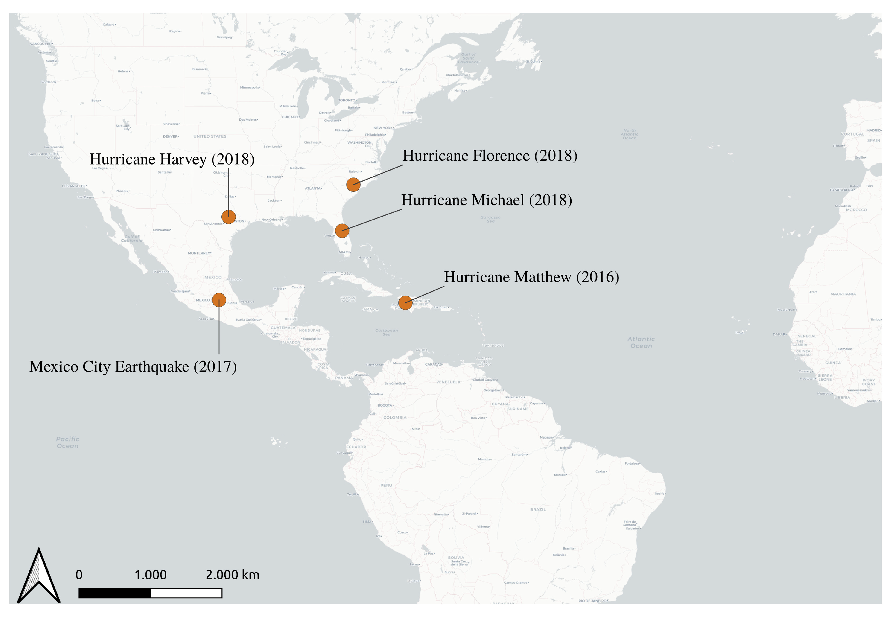
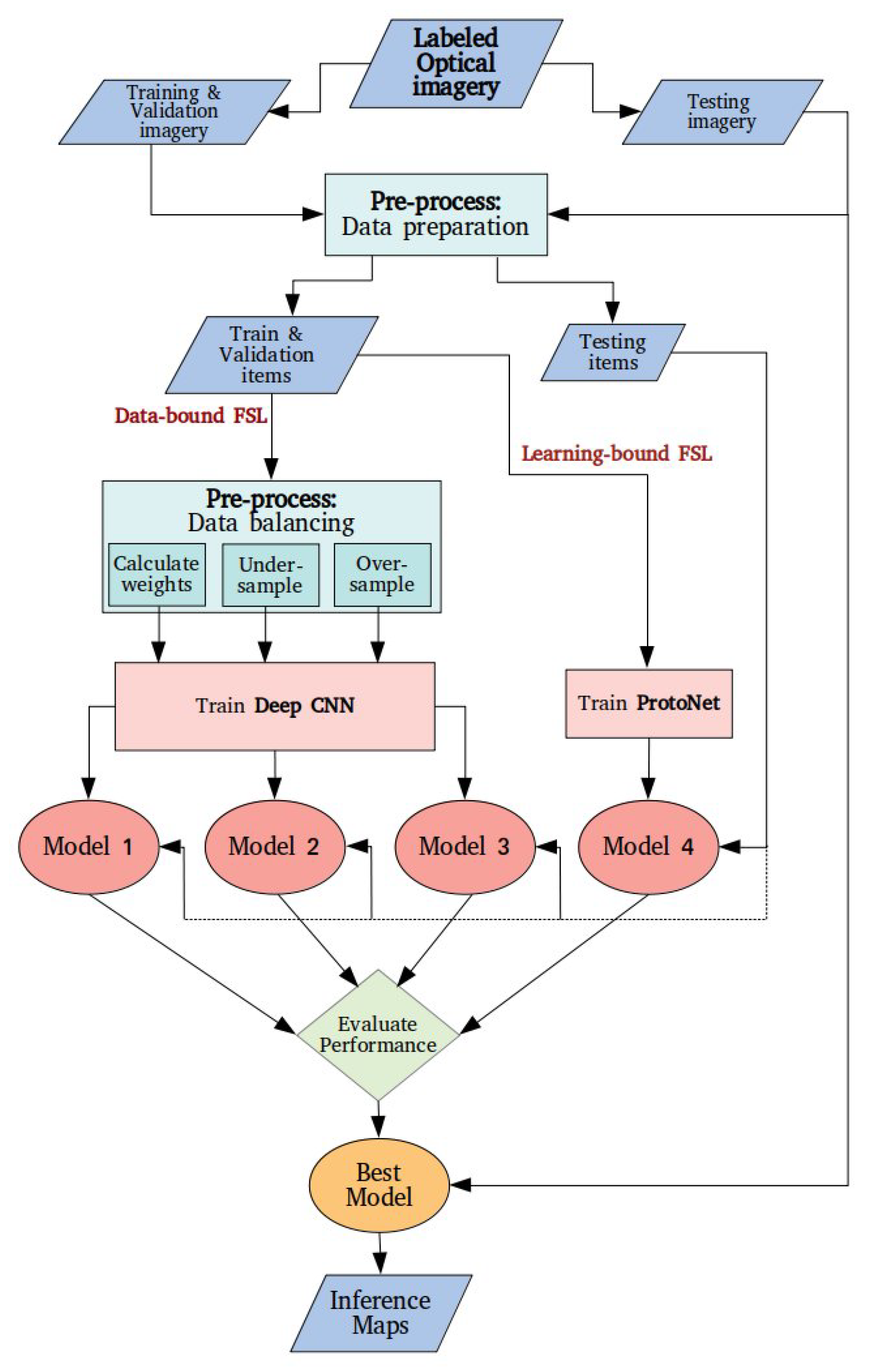
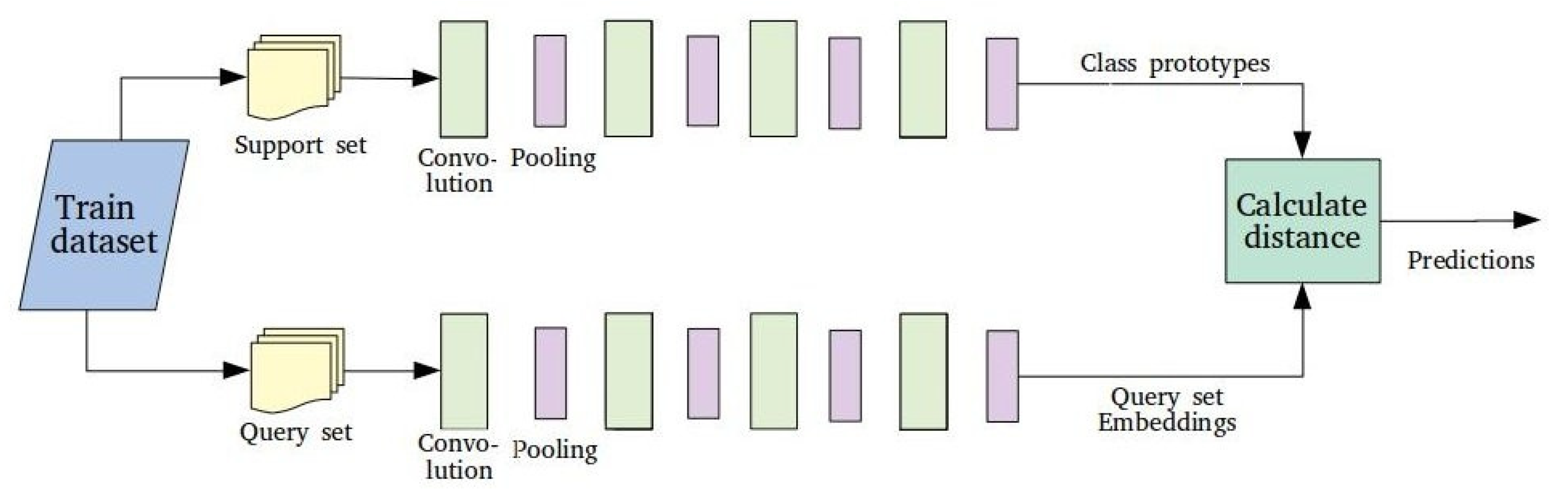
Previous work indicates that the common trend for urban damage assessment with Remote Sensing is to use Deep Learning. The data shortage is mostly addressed with data augmentation, but pre-trained models and unsupervised learning have also been put to the test. All these approaches are considered Few-Shot Learning, demonstrating the applicability of this Machine Learning family of strategies in relevant problems. In this study, we took into consideration the type of input imagery (labeled optical imagery) and the intended number of output classes (four-level damage scale) to select the appropriate methodological components. According to the conclusions drawn by the literature review, we confronted the data shortage in two distinct ways: (1) balancing and augmenting the dataset to make it suitable for training a Deep Architecture and (2) metric Few-Shot Learning with Prototypical Networks. More data from hurricane incidents were incorporated in the analysis as a first step of expanding the dataset with data from related problems. Subsequently, four different models were developed and compared.

As revealed by the quantitative evaluation to which the models were subjected, oversampling achieved the highest precision and f-score values for all classes and the highest recall values for all classes except Minor damage, amongst all three data-balancing strategies for Deep Learning architectures. This outcome is consistent with related studies that have used the xBD dataset for model training. Valentijn et al. [14] have compared cost-sensitive learning with a combination of over and undersampling and conclude that the latter is more effective in the classification outcome. Bai et al. [15] mention that after preliminary experiments, they chose to use oversampling to train their models. Contrarily Ji et al. [6] used a different dataset to train a binary CNN-based classifier and found cost-sensitive learning more effective as a balancing operation.

The comparison of the four models demonstrates that Prototypical Network models can outperform Deep Learning models in damage classification problems with data scarcity. However, in accordance with other studies from the literature, it was not easy to acquire very high accuracy results for a small dataset with slight inter-class disparities in a multi-class classification task. Furthermore, although the xBD dataset is not uncommon in the recent damage classification studies, its use of it in research that focuses on FSL has not been encountered in the literature. As a consequence, similar studies exploit the entirety of the xBD for model training. Valentijn et al. [14], who trained a model based on Inception-v3 with xBD, report on recall as the following: No damage: 0.867, Minor damage: 0.541, Major damage: 0.607 and Destroyed: 0.679. As shown in Table 9, the recall of the ProtoNets model is 0.69 for No damage, 0.52 for Minor damage, 0.57 for Major damage and 0.75 for Destroyed. The results are not only comparable but also can surpass the performance of a model trained with the entire dataset. Bai et al. [15], who also trained their proposed architecture with xBD, report on the same evaluation metrics as the present paper, namely precision, recall and f-score, and distinguish between localization and classification metrics, so the comparison with the values of Table 9 is more straight-forward. For No damage, the results for precision, recall and f-score are 90.64%, 87.07% and 89.85%, respectively, and are significantly higher than the respective values in Table 9. On the contrary, the calculated metrics for Minor damage (precision: 35.51%, recall: 49.50%, f-score: 41.36%) are significantly lower than the values of Table 9. For Major damage, the Bai et al. [15] performance metrics (precision: 65.80%, recall: 64.93%, f-score: 65.36%) are higher than Model 4. Finally, for Destroyed, the precision in Bai et al. [15] is 87.08%, which is higher than Model 4, but the other two metrics (recall: 57.87%, f-score: 69.55%) are lower than Model 4. As a general remark, Model 4, which is based on ProtoNets, exhibits more consistent behavior across the four classes, but it performs significantly lower for No damage.

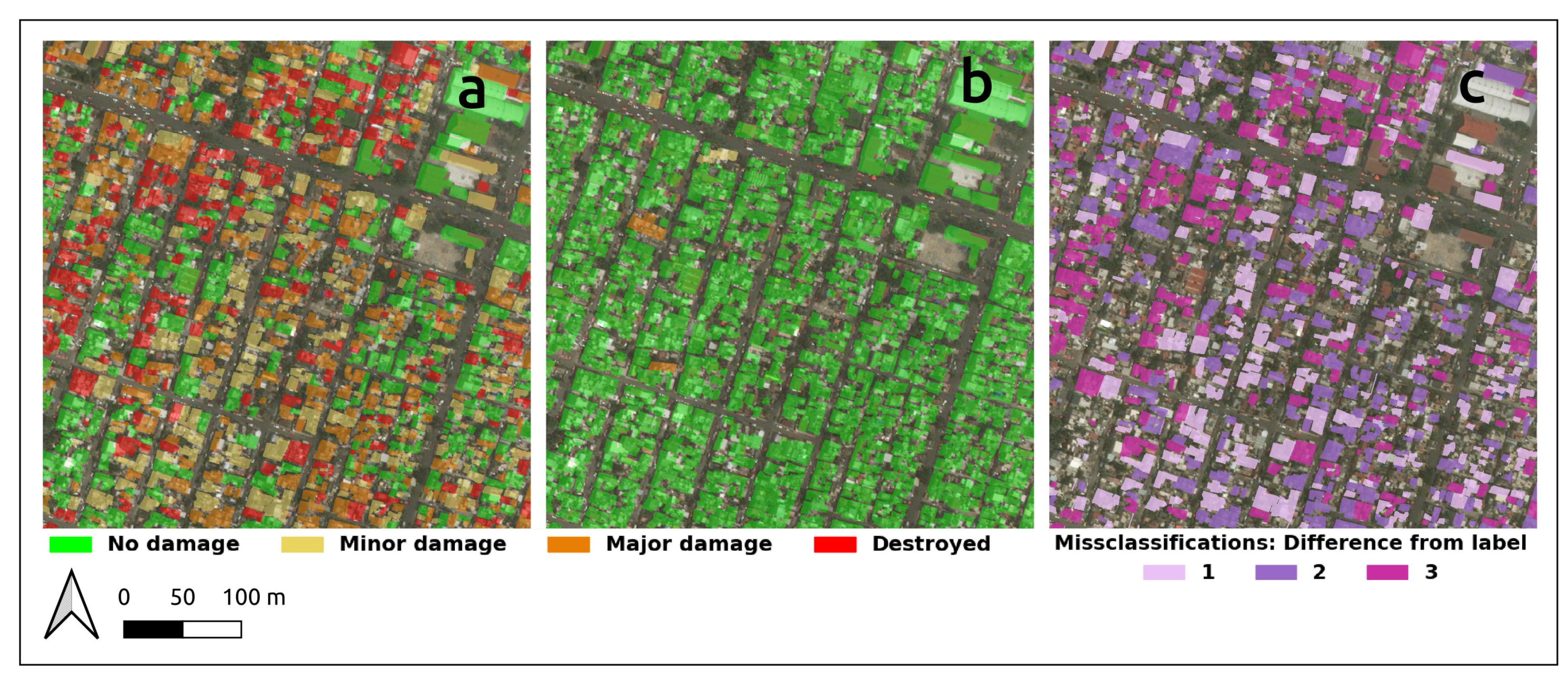
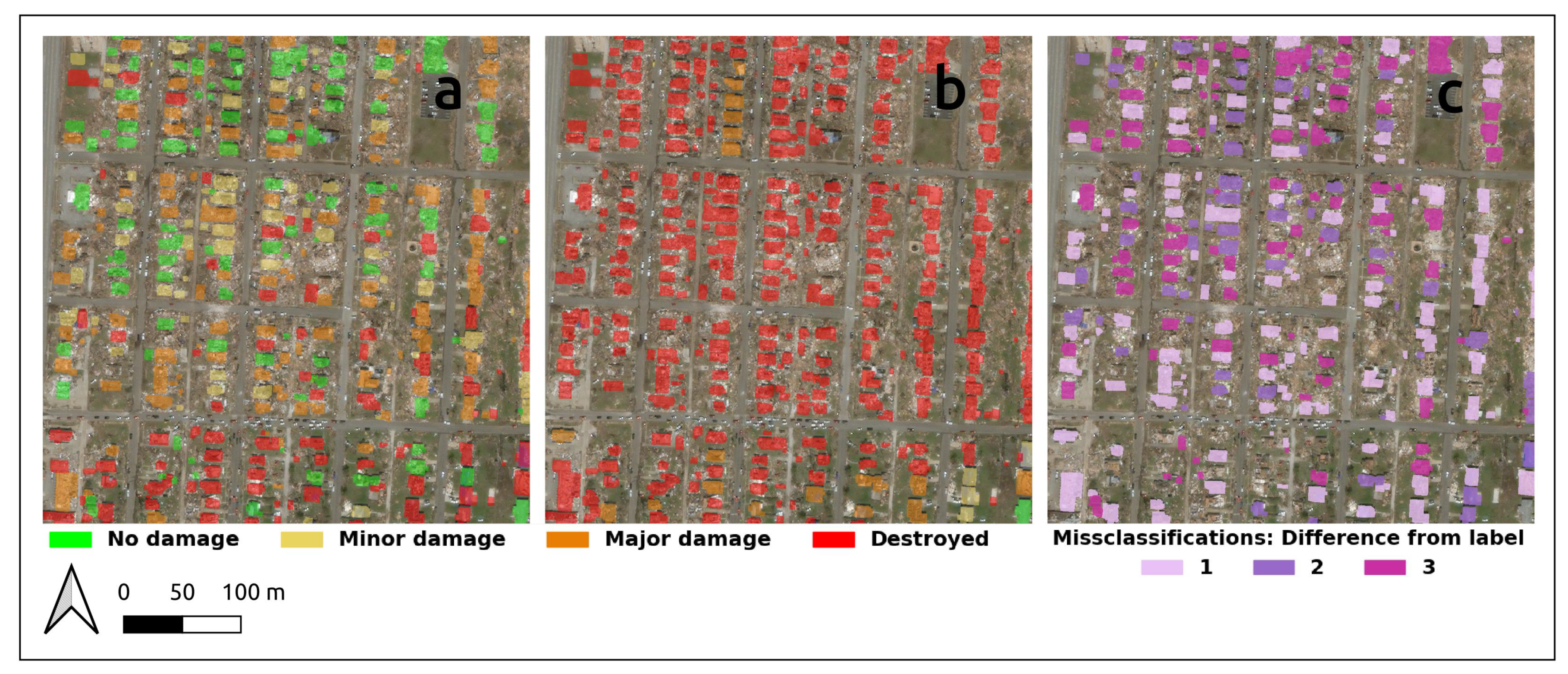
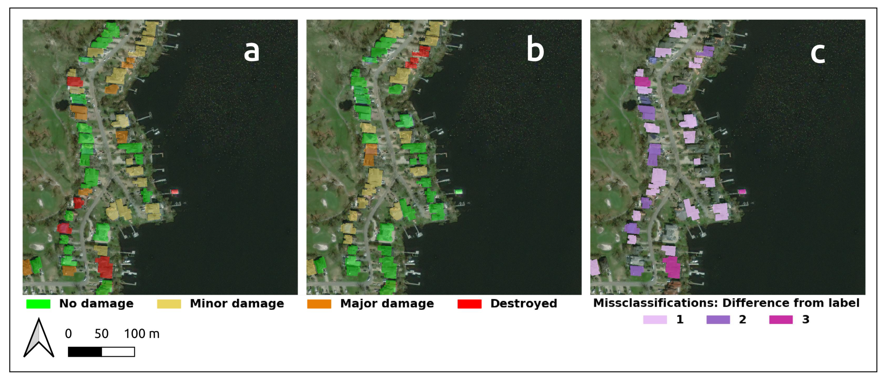
Based on the intuitive interpretation gained by the visual mapping of the predictions of Model 4 compared to the ground truth, we can deduce that the tested model has plenty of room for improvement but seems promising for tackling the problem of post-earthquake urban damage assessment. The most confounding aspect of the results is when No damage buildings are misinterpreted as Destroyed and vice versa because in a real case scenario it could lead to consuming critical resources and time for assisting the wrong locations. It must be stated that such misclassifications seem to be more rare as the area of the polygon increases. In the broader context of emergency response, the significance of the damage classification output should be validated by other data sources. Seismic vulnerability reports, smart building structural monitoring [46] and earthquake magnitude measurements based on environmental noise [4] can be ancillary information to earth observation-based damage classification. The aforementioned information sources, along with ground-truth verification, should be taken into account for the response planning by the local authorities, as the traffic network capacity and the citizen mobility demands change dramatically during the recovery process [16].

While the obtained results from Model 4 seem promising, there are certain limitations to the extent a 50-shot metric-learning approach on satellite imagery of this resolution can reach. Randomly picking 50 representatives of each class to train a ProtoNet model may have led to excluding important information carried by the data. Additionally, satellite imagery of higher resolution is usually private, and thus, very difficult to acquire. The model’s ability to assess damage is also limited to disasters of a magnitude similar to the events in the training data set.

Since the outcome is encouraging, further research on this subject is recommended. Although remotely sensed imagery of higher resolution is difficult to obtain, we anticipate that a similar study with satellite or UAV imagery of higher resolution should be pursued. UAVs can also provide oblique perspectives of the buildings, which may hold important information in the context of structural damage and have been already applied in similar applications [7]. Furthermore, instead of picking at random a few examples from the available data, certain data sampling techniques, such as Near-Miss and Condensed Nearest Neighbor Rule, can be employed to determine the most useful samples to train a model. We strongly believe that Prototypical Networks in the context of urban damage assessment deserve more exploration. The number of shots, the prototyping function and the distance function are parameters to experiment with, and that could improve the existing results.

6. Conclusions

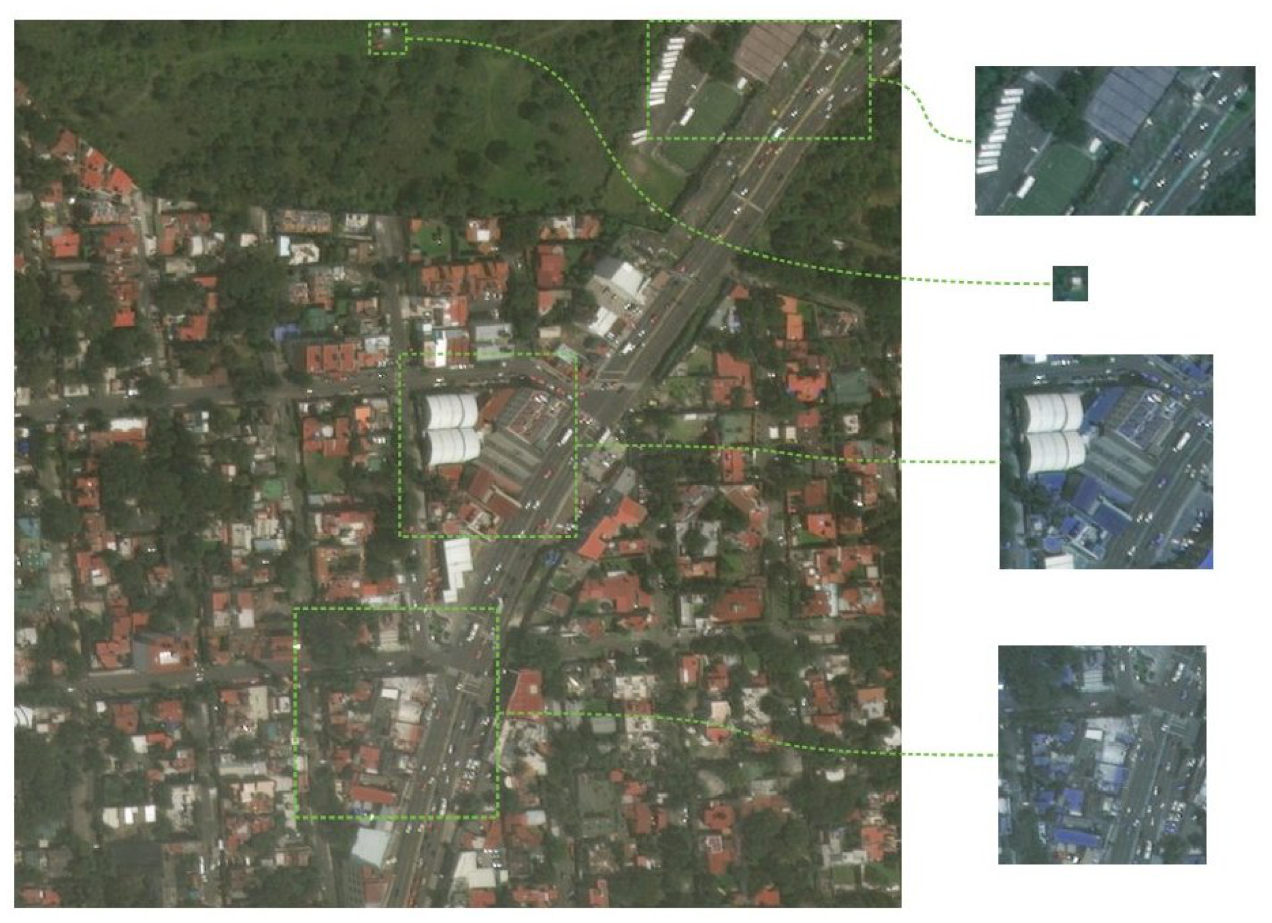
This study employed Very-High Resolution pan-sharpened satellite imagery and Machine Learning in order to identify the level of structural destruction induced by a catastrophic earthquake incident. Aiming to approximate a real case scenario, where the available labeled post-event data are limited, and the pre-event data are possibly nonexistent, the different explored possibilities tackle data insufficiency and imbalance by implementing Few-Shot Learning strategies and pave the way for a new approach to the difficult problem of multi-class damage classification that is formulated upon limited data.

The classification of an imbalanced dataset can be solved either by adjusting the weight matrix, in a way trying to normalize the number of examples for every class (cost-sensitive learning) or by selecting the same number of representatives for each class to build the training set. For a balanced Deep CNN training, three different models were created: Model 1 with cost-sensitive learning, Model 2 with undersampling and Model 3 with oversampling. For Model 4, a 50-shot ProtoNet was trained. This process resulted in four models, each having been trained with a different dataset in terms of the total number of examples and the class proportions. Nevertheless, all models were evaluated based on the same balanced set of completely unseen data. The first method was eventually inefficient in our case while using a balanced dataset when training image classification models immediately added up to the overall performance. Undersampling may cause a loss of decisive information for the classification process, and thus, it is not as considerable as oversampling for training a Deep CNN model. However, for Prototypical Networks, randomly picking a few samples per class was enough for creating the most effective and efficient model.

The four models were compared using precision, recall and f-score. Model 4, built upon Prototypical Networks, showed the most consistent performance according to the three metrics, although Model 3 (data oversampling in the pre-processing stage) exhibited almost equally good results for most classes. Taking a closer look, all four approaches have a different impact on each class. It can be argued that such an eminently imbalanced dataset cannot fully support the training of a multi-class predictive model with cost-sensitive learning since Model 1 is entirely unable to detect the minority class. As stated before, undersampling also leads to dismissing valuable information and hence, the resulting Model 2 has a limited predictive ability over certain classes but performs very well for the minority class. Oversampling seems to be more competent for creating a Deep CNN-based predictive model but has a borderline performance for the majority class. Model 4 seems to achieve a robust performance for all classes, being able to correctly predict more than half of their instances. Consequently, Model 4 was used for creating damage assessment maps to provide an idea of the model’s practical applicability.

The predictions of Model 4 were overlaid with the satellite imagery and compared with the true polygon labels to obtain a qualitative impression of how close the output of the model is to reality. Even though the model is in the right direction for damage assessment, it would not be advisable to base on it an estimation about how gravely an area was affected (Figure 6, Figure 7 and Figure 8). Improvements must still be made so that the possible misinterpretations between No damage and Destroyed buildings are eliminated. This phenomenon seems less frequent for polygons of a larger area.

References

1. Centre for Research on the Epidemiology of Disasters (CRED); UN Office for Disaster Risk Reduction (UNDRR). Human Cost of Disasters: An Overview of the Last 20 Years (2000–2019); Technical Report; CRED: Brussels, Belgium; UNDRR: Geneva, Switzerland, 2020. [Google Scholar]
2. Mitchell, T. Machine Learning, 1st ed.; McGraw-Hill: New York, NY, USA, 1997. [Google Scholar]
3. Harirchian, E.; Kumari, V.; Jadhav, K.; Rasulzade, S.; Lahmer, T.; Raj Das, R. A Synthesized Study Based on Machine Learning Approaches for Rapid Classifying Earthquake Damage Grades to RC Buildings. Appl. Sci. 2021, 11, 7540. [Google Scholar] [CrossRef]
4. Mężyk, M.; Chamarczuk, M.; Malinowski, M. Automatic Image-Based Event Detection for Large-N Seismic Arrays Using a Convolutional Neural Network. Remote Sens. 2021, 13, 389. [Google Scholar] [CrossRef]
5. Cooner, A.J.; Shao, Y.; Campbell, J.B. Detection of urban damage using remote sensing and machine learning algorithms: Revisiting the 2010 Haiti earthquake. Remote Sens. 2016, 8, 868. [Google Scholar] [CrossRef] [Green Version]
6. Ji, M.; Liu, L.; Buchroithner, M. Identifying collapsed buildings using post-earthquake satellite imagery and convolutional neural networks: A case study of the 2010 Haiti Earthquake. Remote Sens. 2018, 10, 1689. [Google Scholar] [CrossRef] [Green Version]
7. Vetrivel, A.; Gerke, M.; Kerle, N.; Nex, F.; Vosselman, G. Disaster damage detection through synergistic use of deep learning and 3D point cloud features derived from very high resolution oblique aerial images, and multiple-kernel-learning. ISPRS J. Photogramm. Remote Sens. 2018, 140, 45–59. [Google Scholar] [CrossRef]
8. Anniballe, R.; Noto, F.; Scalia, T.; Bignami, C.; Stramondo, S.; Chini, M.; Pierdicca, N. Earthquake damage mapping: An overall assessment of ground surveys and VHR image change detection after L’Aquila 2009 earthquake. Remote Sens. Environ. 2018, 210, 166–178. [Google Scholar] [CrossRef]
9. Xu, J.Z.; Lu, W.; Li, Z.; Khaitan, P.; Zaytseva, V. Building Damage Detection in Satellite Imagery Using Convolutional Neural Networks. arXiv 2019, arXiv:1910.06444. [Google Scholar]
10. Li, Y.; Hu, W.; Dong, H.; Zhang, X. Building damage detection from post-event aerial imagery using single shot multibox detector. Appl. Sci. 2019, 9, 1128. [Google Scholar] [CrossRef] [Green Version]
11. Gupta, R.; Hosfelt, R.; Sajeev, S.; Patel, N.; Goodman, B.; Doshi, J.; Heim, E.; Choset, H.; Gaston, M. xBD: A Dataset for Assessing Building Damage from Satellite Imagery. arXiv 2019, arXiv:1911.09296. [Google Scholar]
12. Ji, M.; Liu, L.; Zhang, R.; Buchroithner, M.F. Discrimination of earthquake-induced building destruction from space using a pretrained CNN model. Appl. Sci. 2020, 10, 602. [Google Scholar] [CrossRef] [Green Version]
13. Li, Y.; Lin, C.; Li, H.; Hu, W.; Dong, H.; Liu, Y. Unsupervised domain adaptation with self-attention for post-disaster building damage detection. Neurocomputing 2020, 415, 27–39. [Google Scholar] [CrossRef]
14. Valentijn, T.; Margutti, J.; van den Homberg, M.; Laaksonen, J. Multi-Hazard and Spatial Transferability of a CNN for Automated Building Damage Assessment. Remote Sens. 2020, 12, 2839. [Google Scholar] [CrossRef]
15. Bai, Y.; Hu, J.; Su, J.; Liu, X.; Liu, H.; He, X.; Meng, S.; Mas, E.; Koshimura, S. Pyramid Pooling Module-Based Semi-Siamese Network: A Benchmark Model for Assessing Building Damage from xBD Satellite Imagery Datasets. Remote Sens. 2020, 12, 4055. [Google Scholar] [CrossRef]
16. Costa, C.; Figueiredo, R.; Silva, V.; Bazzurro, P. Application of open tools and datasets to probabilistic modeling of road traffic disruptions due to earthquake damage. Earthq. Eng. Struct. Dyn. 2020, 49, 1236–1255. [Google Scholar] [CrossRef]
17. Boccardo, P.; Tonolo, F.G. Remote sensing role in emergency mapping for disaster response. In Engineering Geology for Society and Territory—Volume 5: Urban Geology, Sustainable Planning and Landscape Exploitation; Springer International Publishing: Cham, Switzerland, 2015; pp. 17–24. [Google Scholar] [CrossRef]
18. Kakooei, M.; Baleghi, Y. Fusion of satellite, aircraft, and UAV data for automatic disaster damage assessment. Int. J. Remote Sens. 2017, 38, 2511–2534. [Google Scholar] [CrossRef]
19. Maxwell, A.E.; Warner, T.A.; Fang, F. Implementation of machine-learning classification in remote sensing: An applied review. Int. J. Remote Sens. 2018, 39, 2784–2817. [Google Scholar] [CrossRef] [Green Version]
20. Wang, Y.; Yao, Q.; Kwok, J.; Ni, L.M. Generalizing from a Few Examples: A Survey on Few-Shot Learning. ACM Computing Surveys (CSUR) 2020, 53, 1–34. [Google Scholar] [CrossRef]
21. Kadam, S.; Vaidya, V. Review and analysis of zero, one and few shot learning approaches. In Proceedings of the 18th International Conference on Intelligent Systems Design and Applications (ISDA 2018), Vellore, India, 6–8 December 2018; Volume 940, pp. 100–112. [Google Scholar] [CrossRef]
22. Branco, P.; Torgo, L.; Ribeiro, R. A Survey of Predictive Modelling under Imbalanced Distributions. arXiv 2015, arXiv:1505.01658. [Google Scholar]
23. Ge, P.; Gokon, H.; Meguro, K. A review on synthetic aperture radar-based building damage assessment in disasters. Remote Sens. Environ. 2020, 240, 111693. [Google Scholar] [CrossRef]
24. Li, K.; Wan, G.; Cheng, G.; Meng, L.; Han, J. Object detection in optical remote sensing images: A survey and a new benchmark. ISPRS J. Photogramm. Remote Sens. 2020, 159, 296–307. [Google Scholar] [CrossRef]
25. Taher, R. General Recommendations for Improved Building Practices in Earthquake and Hurricane Prone Areas; Technical Report; Architecture for Humanity: San Francisco, CA, USA, 2010. [Google Scholar]
26. Fannela, D.A.; Munshi, J.A. Design of Concrete Buildings for Earthquake & Wind Forces According to the 1997 Uniform Building Code, 1st ed.; Portland Cement Association: Skokie, IL, USA, 1998. [Google Scholar]
27. Deng, J.; Dong, W.; Socher, R.; Li, L.J.; Li, K.; Li, F.-F. ImageNet: A large-scale hierarchical image database. In Proceedings of the 2009 IEEE Conference on Computer Vision and Pattern Recognition, Miami, FL, USA, 20–25 June 2009; pp. 248–255. [Google Scholar] [CrossRef] [Green Version]
28. Weber, E.; Kané, H. Building Disaster Damage Assessment in Satellite Imagery with Multi-Temporal Fusion. Remote Sens. 2019, 11, 2765. [Google Scholar] [CrossRef] [Green Version]
29. Touzani, S.; Granderson, J. Open Data and Deep Semantic Segmentation for Automated Extraction of Building Footprints. Remote Sens. 2021, 13, 2578. [Google Scholar] [CrossRef]
30. Choi, W.G.; Lee, K.S. Conceptual representation for crisis-related tweet classification. Comput. y Sist. 2019, 23, 1523–1531. [Google Scholar] [CrossRef]
31. Balamurugan, A.; Zakhor, A. Online Learning for Indoor Asset Detection. In Proceedings of the 2019 IEEE 29th International Workshop on Machine Learning for Signal Processing (MLSP), Pittsburgh, PA, USA, 13–16 October 2019. [Google Scholar] [CrossRef]
32. Liu, K.; Liu, W.; Ma, H.; Huang, W.; Dong, X. Generalized zero-shot learning for action recognition with web-scale video data. World Wide Web 2019, 22, 807–824. [Google Scholar] [CrossRef] [Green Version]
33. Maxar. Open Data Program|Disaster Response Geospatial Analytics. Available online: https://www.maxar.com/open-data (accessed on 9 October 2021).
34. Grünthal, G.; Musson, R.; Schwarz, J.; Stucci, M. European Macroseismic Scale 1998 (EMS-98); Technical Report; European Centre for Geodynamics and Seismology: Luxembourg, 1998. [Google Scholar]
35. He, K.; Zhang, X.; Ren, S.; Sun, J. Deep residual learning for image recognition. In Proceedings of the IEEE Conference on Computer Vision and Pattern Recognition, Las Vegas, NV, USA, 27–30 June 2016; pp. 770–778. [Google Scholar] [CrossRef] [Green Version]
36. Fernández, A.; García, S.; Galar, M.; Prati, R.C.; Krawczyk, B.; Herrera, F. Learning from Imbalanced Data Sets; Springer International Publishing: Cham, Switzerland, 2018. [Google Scholar] [CrossRef]
37. Sklearn API Documentation. Available online: https://scikit-learn.org/stable/modules/generated/sklearn.utils.class_weight.compute_class_weight.html (accessed on 22 March 2021).
38. Kingma, D.P.; Ba, J. Adam: A Method for Stochastic Optimization. arXiv 2017, arXiv:1412.6980. [Google Scholar]
39. Snell, J.; Twitter, K.S.; Zemel, R.S. Prototypical Networks for Few-Shot Learning. In Proceedings of the 31st International Conference on Neural Information Processing Systems, Long Beach, CA, USA, 4–9 December 2017. [Google Scholar]
40. Vanschoren, J. Meta-Learning: A Survey. arXiv 2018, arXiv:1810.03548. [Google Scholar]
41. Waldner, F.; Chen, Y.; Lawes, R.; Hochman, Z. Needle in a haystack: Mapping rare and infrequent crops using satellite imagery and data balancing methods. Remote Sens. Environ. 2019, 233, 111375. [Google Scholar] [CrossRef]
42. Sokolova, M.; Japkowicz, N.; Szpakowicz, S. Beyond Accuracy, F-Score and ROC: A Family of Discriminant Measures for Performance Evaluation. In AI 2006: Advances in Artificial Intelligence; Sattar, A., Kang, B.H., Eds.; Springer: Berlin/Heidelberg, Germany, 2006; pp. 1015–1021. [Google Scholar]
43. USAID. Mexico Earthquake Fact Sheet #1—09-21-2017; Technical Report; USAID: Washington, DC, USA, 2017. [Google Scholar]
44. Wagenmaker, R.; Weaver, J.; Garnet, G.; Perry, B.; Spinney, J. NWS Central Region Service Assessment; Technical Report; National Oceanic and Atmospheric Administration, U.S. Department of Commerce: Kansas City, MO, USA, 2011. [Google Scholar]
45. NOAA’s National Weather Service, US Department of Commerce. Catastrophic Hurricane Michael Strikes Florida Panhandle October 10, 2018; Technical Report; Weather Forecast Office: Tallahassee, FL, USA, 2018. [Google Scholar]
46. Serrano, W. iBuilding: Artificial Intelligence in Intelligent Buildings. Neural Comput. Appl. 2021. [Google Scholar] [CrossRef]
Figure 1. The disaster incidents in the training dataset.
Remotesensing 14 00040 g001
Figure 2. Methodology overview.
Remotesensing 14 00040 g002
Figure 3. Isolation of labeled building instances.
Remotesensing 14 00040 g003
Figure 4. Deep Neural Network baseline architecture.
Remotesensing 14 00040 g004
Figure 5. Methodological Workflow and Network Architecture for Model 4.
Remotesensing 14 00040 g005
Figure 6. Application of ProtoNet model on a test case from Mexico 2017. Satellite image overlaid with: (a) the predictions, (b) the labels and (c) the difference between the two.
Remotesensing 14 00040 g006
Figure 7. Application of ProtoNet model on a test case from tornado Joplin. Satellite image overlaid with: (a) the predictions, (b) the labels and (c) the difference between the two.
Remotesensing 14 00040 g007
Figure 8. Application of ProtoNet model on a test case from Hurricane Michael. Satellite image overlaid with: (a) the predictions, (b) the labels and (c) the difference between the two.
Remotesensing 14 00040 g008