Abstract
The ecosystem performance approach, used in a previously published case study focusing on the Nebraska Sandhills, proved to minimize impacts of non-climatic factors (e.g., overgrazing, fire, pests) on the remotely-sensed signal of seasonal vegetation greenness resulting in a better attribution of its changes to climate variability. The current study validates the applicability of this approach for assessment of seasonal and interannual climate impacts on forage production in the western United States semi-arid grasslands. Using a piecewise regression tree model, we developed the Expected Ecosystem Performance (EEP), a proxy for annual forage production that reflects climatic influences while minimizing impacts of management and disturbances. The EEP model establishes relations between seasonal climate, site-specific growth potential, and long-term growth variability to capture changes in the growing season greenness measured via a time-integrated Normalized Difference Vegetation Index (NDVI) observed using a Moderate Resolution Imaging Spectroradiometer (MODIS). The resulting 19 years of EEP were converted to expected biomass (EB, kg ha−1 year−1) using a newly-developed relation with the Soil Survey Geographic Database range production data (R2 = 0.7). Results were compared to ground-observed biomass datasets collected by the U.S. Department of Agriculture and University of Nebraska-Lincoln (R2 = 0.67). This study illustrated that this approach is transferable to other semi-arid and arid grasslands and can be used for creating timely, post-season forage production assessments. When combined with seasonal climate predictions, it can provide within-season estimates of annual forage production that can serve as a basis for more informed adaptive decision making by livestock producers and land managers.
1. Introduction
Rangelands in the United States cover around 312 million ha representing about 30% of the total land area [1]. Climatic changes, including more frequent and longer-duration droughts and long-term directional shifts in temperature and precipitation seasonality and amounts, can substantially affect forage production [2,3,4,5]. Reduced forage production can lead to lower livestock gains, soil erosion, water quality and quantity issues, and often results in rippling socio-economic impacts like physical and emotional stress [6] or financial and social instability [7]. For example, a widespread severe drought in 2012 led to poor or very poor conditions in 59% of the total U.S. pasture and range areas [8], costing taxpayers over $2.6 billion through record payouts via the U.S. Department of Agriculture’s Livestock Forage Program [9]. Despite this drought assistance, many producers experienced losses in welfare that may have persisted for several years [10].
Semi-arid rangelands of the United States have inherently high interannual differences in forage production mostly connected to inter- and intra-annual variability in precipitation [11,12,13]. Matching animal demand to forage availability using adaptive management can improve animal weight gains [14] and increase sustainability of land management. Previous management emphasized fixed moderate to low stocking rates, based on decadal-scale research, that optimized weight gains per animal and per unit land area [15] with slow but substantial changes to these stocking rates over long periods of time (e.g., multiple decades) [16]. These fixed stocking rates result in underutilization of forage during years with above-average forage production while also creating difficult and costly grazing management decisions to reduce numbers of livestock or shorten the grazing season in drought years. The use of flexible stocking rates, adjusted seasonally/annually based on forage availability, provides opportunities for more efficient utilization of available forage within and across years and can be advantageous for economic returns [17,18,19,20].
A fundamental need for producer decision-making using adaptive management and flexible stocking rates is the accurate simulation or prediction of forage production prior to and during the grazing season. Modeling efforts are available but the complexity of plant communities in rangelands remains challenging for site-level estimates [21] and cross-site efforts are more problematic [22]. Lack of large-scale, long-term, coordinated ground observations of forage production hinders development of a robust model covering large spatial extents that would rely solely on ground-observed data. Alternatively, advancements in remote sensing and processing of big data have produced emergent tools in the United States for estimating forage production in rangelands at large spatial scales with enhanced accuracy (Table 1). These tools can be generally categorized into two groups based on the timing of the provided information: (1) a post-growing season assessment and (2) a within-growing season prediction of annual forage yield. Characteristics and limitations of these tools are provided in Table 1.

Table 1.
Characteristics of large-scale rangeland forage production prediction tools in the United States.
Except for the SDDT, all the tools identified in Table 1 in some way use satellite-observed Normalized Difference Vegetation Index (NDVI, [27]) data for estimating forage production. While effectively capturing spatial and temporal patterns of greenness, vegetation health, and annual biomass production [28,29,30], NDVI and tools using NDVI do not provide information about the underlying causes of changes in grassland productivity [31].
Many factors affect forage production across spatial and temporal scales. Long-term spatial patterns of forage production are primarily affected by soil characteristics, vegetation type, long-term climate, and topography [11,32,33]. Temporal scale variability, in contrast, is driven primarily by the intra- and interannual variability in climate conditions [12,13,34,35], fire [36], pest outbreaks [37], management [13], and growing conditions of the previous year [38,39]. To limit the focus to the effect of intra- and inter-annual climate variability on forage production, other non-climatic effects that cause variability in forage production during the growing season, such as disturbances caused by overgrazing, fire, flooding, and pests, would need to be minimized or eliminated completely. In a case study from the Nebraska Sandhills, the Expected Ecosystem Performance (EEP) approach [40] was used to separate the climate signal from other annual effects [3]. The amount of expected forage production was estimated solely based on seasonal climate and site-specific characteristics using a data-driven piecewise regression tree model. This model used a long-term historical NDVI dataset at 250-m spatial and weekly temporal resolutions as a proxy for annual forage production. While the approach was successful in estimating annual forage production based on observed climate, the model was developed over a specific and relatively small ecoregion.
Here, we test the extension of the EPP approach with the piecewise regression tree model on semi-arid grasslands of the western United States. The objectives are as follows: (1) develop an EEP model and historical maps of EEP derived from this model for the years 2000 until 2018 that retain the information from the climate signal but reduce other non-climatic factors, (2) convert the EEP to a measure of forage biomass (e.g., kg ha−1), (3) assess the accuracy of EEP estimates across various sites within the study area using independent ground-based observations, and (4) test whether the model can be used beyond the model training period (2000–2018). The outcome of our efforts was to ascertain the applicability of EEP for post-growing season assessments and, if used in conjunction with seasonal climate forecasts or scenarios, for timely within-growing season annual forage predictions.
2. Site Description
The spatial extent of the study and resulting biomass maps cover major grassland areas in western United States (Figure 1). The eastern border of the study area was determined using the Level II Omernik ecoregion classification [41] that divides the Great Plains into west-central and south-central semi-arid prairies from temperate prairies. Most of the tallgrass temperate prairies, characterized by higher precipitation amounts and resultant greater soil moisture content, were excluded from the analysis because the majority of this grassland type has been converted to cultivated crop land [42]. The western border of the study area is delineated by the mountain ranges of the Sierra Nevada and Cascade Range and the coinciding Level III Omernik ecoregions [41]. We excluded desert ecoregions including the Mojave Basin and Range, Sonoran Basin and Range, Arizona-New Mexico Plateau, and Chihuahuan Desert, where growth dynamics of sparse vegetation cover are difficult for moderate resolution sensors to detect. We divided the study site into two regions that differ in the percentage of herbaceous land cover compared to other land cover classes in each Level III ecoregion (Figure 1). More detailed description of the differences between these two regions is provided in Appendix A. The study site has a total area of over 3 million km2 and is diverse in climate, elevation, soil properties, and land cover types. Annual precipitation ranges from ~100 mm to 2500 mm, the minimum February temperature from −19 to 11 °C, and the maximum August temperature from 13 to 38 °C. As summarized in The Fourth National Climate Assessment [43], over the last few decades the western part of the United States has seen the largest increases in annual temperatures (over 0.8 °C) when compared to the entire United States. Since the beginning of the 20th century, the United States has experienced changes in precipitation patterns with increases in annual mean precipitation in the Midwest and Great Plains and decreases in the Southwest. These trends are expected to continue in the future [43]. Elevation in the study site ranges from ~30 m to 4300 m. The soil orders include, but are not limited to, Mollisols, Entisols, Aridisols, and Alfisols. Most of the area is well drained, while some locations are somewhat excessively drained (e.g., Nebraska Sandhills). Although the area contains many different Land Cover (LC) classes, we focused purely on the grassland/herbaceous class as identified in the National Land Cover Database 2016 (NLCD 2016). Because of the large geographic extent of the study area, livestock management strategies vary based on location-specific characteristics.
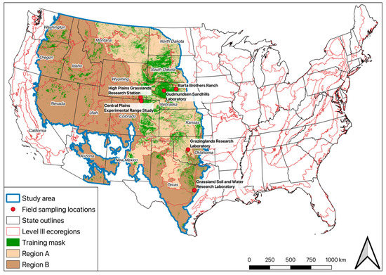
Figure 1.
Location of the study area. Region A represents the Great Plains with higher percentage of herbaceous cover, while Region B represents the southern and western areas with much lower total herbaceous cover. The green areas display the distribution of areas that were identified as suitable for placement of model training points. Locations of ground-based validation are displayed as red dots.
3. Methods
This study builds upon the methods used in a proof-of-concept study by Poděbradská et al. [3]. We introduce the forage production model methodology but focus primarily on the adjustments made to the methodology of Poděbradská et al. [3] with emphasis on additional steps necessary for regional application at that larger scale that is more variable in climate, land cover, elevation, and land use.
A data-driven, rule-based Regression Tree (RT) model is used to estimate annual forage production based on a combination of remotely sensed site-specific characteristics and seasonal climate data [3]. RT models provide an accurate representation of complex systems and bring insight to non-linear relations and higher-order interactions that occur between the dependent and independent variables [40]. In RT models, the input data space is stratified into several small multi-dimensional zones. In each zone, a linear regression model is fit to predict the dependent variable using some or all of the independent variables. Each zone is then represented by the definition of the zone (similar to decisions trees) and a corresponding regression equation [44].
The output of our RT model is the EEP, which represents a proxy for the total annual biomass expected to be produced at a specific location under certain climate conditions, omitting other influencing factors like management, fire, or pests, which are not model input variables. The ecosystem performance approach was originally developed for boreal forest ecosystems [40] but has been frequently used in grasslands [3,45,46,47,48].
3.1. Model Inputs
The RT model was designed and run using Cubist® software [49]. The target (dependent) variable in the RT model was the Growing Season NDVI (hereon called GSN), a proxy of annual vegetation growth, e.g., [26,50,51]. The NDVI is one of the most widely used vegetation indices capturing changes in vegetation greenness. It uses information about the reflectance of the red and near infrared (NIR) portion of the electromagnetic spectrum (Equation (1)), which can be utilized for assessing vegetation health, drought stress, biomass production, and other vegetation-related information [28,29,30].
The GSN is often approximated using an integral of the NDVI collected multiple times between the start and end dates of the growing season [52,53]. In large geographic areas, the start and end dates of the growing season can vary considerably with location and from year to year. To address this, we developed a method to dynamically approximate the GSN without defining the specific start and end dates of the growing season using archived modified NDVI data obtained from the U.S. Geological Survey Earth Observation and Science Center (USGS EROS). The modified NDVI (mNDVI data) consists of Expedited Moderate Resolution Imaging Spectroradiometer (eMODIS) weekly NDVI composites with 250-m spatial resolution [54] from the MODIS Terra collection 5 (2000–2002) and MODIS Aqua collection 6 (2003–2018) that are quality masked, temporally smoothed [55], and scaled to 0–200. The GSN was calculated as the sum of weekly (n = 52) positive differences (negative differences are omitted) between the mNDVI and the scaled NDVI value 120 (hereafter called the base NDVI), which corresponds to a NDVI of 0.2 (0.2 NDVI * 100 + 100). The base NDVI represents a signal from soil background and dead vegetation [56]. The calculation of the GSN is expressed as:
This approach ensures that the GSN represents forage growth during the growing season, which varies in start, end, and duration based on geographical location, site specific characteristics, and interannual differences in growing conditions.
The independent (explanatory) variables in the model include: seasonal climate data, site potential, and a long-term mean absolute error of the GSN (MAE GSN). Seasonal climate data were calculated from monthly climate variables (minimum, mean, and maximum temperature, and precipitation) obtained from the PRISM Climate Group [57]. Monthly data, available at a 4-km spatial resolution, were bilinearly interpolated to 250 m and converted to seasonal values (winter—December, January, February; spring—March, April, May; summer—June, July, August) depending on the specific variable—mean of 3 months for temperature variables and sum of 3 months for precipitation. Site potential (Figure 2 and Figure A1), defined as the mean of annual GSN values that are higher than long-term GSN median, represents the spatial variability in forage production potential governed by local biogeophysical properties that stay relatively stable across time. This method of site potential approximation has been previously used in grassland areas [3,45]. The MAE GSN (Figure 2) serves as the measure of mean interannual variability in forage growth and has been used in estimates of annual exotic herbaceous cover in the sagebrush ecosystem [58]. These independent variables were selected based on their relationship with plant growth, data availability, and appropriateness of their spatial and temporal resolution. Additionally, these variables correspond to those used in the proof-of-concept case study by Poděbradská et al. [3] and similar studies, e.g., [45,46,47,48,58].
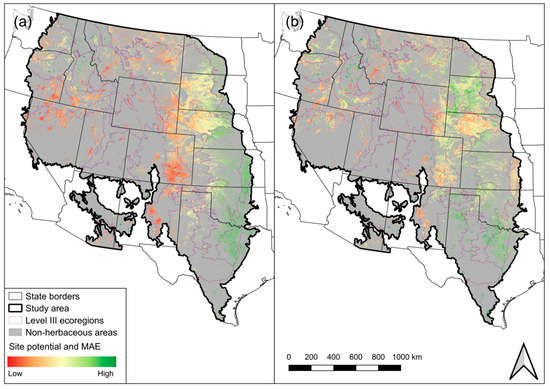
Figure 2.
Distribution of site potential (a) and long-term Mean-Absolute Error (b, MAE) in units of mNDVI across the study area for grassland land cover.
3.2. EEP, EB, Annual Biomass Deviation, and Percent Normal Biomass
The GSN serves as the predicted (dependent) variable in the EEP model. Site potential, the long-term MAE of the GSN, and seasonal climate variables are used as the explanatory (independent) variables (Figure 3). Thus, EEP is solely based on climate and long-term site-specific variations and lacks inputs that would explain EEP variability due to management or disturbances included in the model training database. This facilitates the isolation of climate driven dynamics for the EEP predictions. The number of rules and other model parameters were based on the recommendations of Gu et al. [59] that aim to minimize over- and under-fitting tendencies. Model output, specifically, a set of rules and multiple linear regressions, was further used to develop maps of EEP in MapCubist, an internal USGS EROS code for application of Cubist model output. MapCubist can be substituted with open-source python modules (e.g., GDAL, Pickle) as underlying mapping applications. The method for delineating the area that was used for placement of model training points and displaying of model results is described in Appendix A (Table A1).
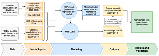
Figure 3.
A flowchart of the inputs and processing steps in development of the Expected Ecosystem Performance (EEP) model and annual maps, conversion to expected biomass and validation of the results.
The rangeland productivity dataset within the Soil Survey Geographic Database (SSURGO, obtained from https://nrcs.app.box.com/v/soils, last accessed on 18 November 2021) was used to convert a unitless EEP to biomass units for producers (Figure 3). Biomass values, typically measured in kg ha−1 or lbs acre−1, are more relevant to rangeland managers and livestock producers than GSN index values. Accordingly, we established a relation between EEP and dry matter biomass values obtained from the SSURGO range production database. The SSURGO database contains three biomass categories that illustrate low, representative, and high production years. We created a dataset of the 25th, 50th, and 75th percentiles from the time-series of annual EEP values (2000–2018) to match these three categories. We extracted SSURGO and EEP values from randomly located points (n = 37,455) within the mapped areas across the three production categories to establish an empirical relation using weighted least squares (WLS) regression (R2 = 0.7), which was used to convert EEP maps into values of Expected Biomass (EB, kg ha−1 yr−1 of dry biomass matter) for each pixel and year. The WLS regression model, which was chosen instead of an ordinary least squares regression due to an observed heteroscedasticity, was fit to the data. The pixel-based EEP was converted to annual biomass values (in kg ha−1) using the resulting regression equation (Equation (3)).
Forage production (kg ha−1 yr−1) = 2.18 ∗ EEP + 340.4
To reduce the observation bias in EEP and SSURGO productivity values, the randomly located points were grouped into 20 clusters of EEP values equally spaced along the range of the values. The mean and standard deviation of the SSURGO productivity was calculated for these clusters. A regression analysis was performed on the cluster EEP and SSURGO data. This approach gives a near-equal importance to data along the entire range of the data values and avoids over- or underestimation biases in the lowest or highest range, which are relatively rare occurrences in the space for time dataset of the regression equation.
The annual biomass deviation was calculated as the EB in a given year minus the long-term biomass median on a pixel basis. The percent anomaly was calculated as the division of EB in a given year by a long-term EB median multiplied by 100. We used the long-term median (as opposed to long-term mean) to calculate the annual biomass deviation and the percent normal biomass. Compared to the mean, the use of the median does not assume the data to be normally distributed and this statistical measure is also less affected by outliers.
We used the Standardized Precipitation Index (SPI, [60]) to qualitatively assess the spatial distribution of abnormally dry and wet conditions and compared it to areas of abnormally high and low biomass production as estimated by the EEP model. Specifically, we used SPI for August 31 with a 6-month time-step that summarizes the moisture conditions over the period of the growing season (from the beginning of March through to the end of August). The SPI data were obtained from https://www.drought.gov/data-maps-tools/us-gridded-standardized-precipitation-index-spi-nclimgrid-monthly (last accessed on 18 November 2021).
3.3. Ground Validation
We obtained long-term ground clipping biomass data from multiple sources for 11 sites in five states of the study region (Figure 1) with details of each found in Table 2. The mean of biomass from multiple clipping locations established in each pasture was used to represent a pasture-wide biomass. The collection of data and the management of the specific data collection pastures differed based on the validation location and its primary research purpose. In some locations exclosure cages were used to completely eliminate grazing pressure on the collected biomass, and in some locations samples were collected from pastures with low grazing pressure, while in others the entire stands were harvested and weighed at the end of the season. These differences can introduce certain inconsistencies when validating the modeled biomass; however, we argue that on a moderate spatial scale these differences are expected to be fairly negligible. The methodology of data collection for each validation site is described in detail in Table 2. We spatially matched the pastures where clipping data were obtained and averaged the pixel biomass values matching the extent of these pastures. A regression and a time-series analysis were performed on the dataset. Data from Texas were excluded from the regression analysis due to a difference in collection methodology (collecting all standing biomass from the stands and weighing non-dried samples), and data from Oklahoma were excluded from the time-series analysis due to a short period of record. We also estimated historical biomass since 1982 (moderate and heavy grazed) and 1991 (light grazed) using our established EB model output by extrapolating the model output using historical climate data and validated these results using long-term ground observations from the USDA Agricultural Research Service research site located near Cheyenne, Wyoming. This site was chosen due to data availability prior to our model training period. We compared the validation results of the historical estimates to estimates created within the model training period (2001–2018). Additionally, we also examined the annual sign of trend (increase/decrease) when compared to a previous year’s production for all locations of modeled and observed data.

Table 2.
Summary of the ground-based observations used for a validation of our modeled results.
4. Results
4.1. Site Potential and MAE GSN
The site potential captured a productivity gradient over the Great Plains from southeast to northwest (Figure 2). The long-term interannual variability captured by the MAE GSN did not follow the same spatial patterns. Lower, long-term interannual variability was observed in the Middle Rockies, Wyoming Basin, Nebraska Sandhills, and Flint Hills. Higher interannual production variability was observed generally in Texas and South Dakota with spots scattered around the entire study area (Figure 2).
4.2. EEP Model
The EEP model was trained on 80% of the total points (n = 277,931) with 20% of the points used for independent model validation. The model was limited to 33 rules and used three committee models (which use mean predictions from multiple model runs to fine-tune the model [63]). Table 3 provides a list of the independent variables used in the model ranked by overall importance and the model evaluation on training and testing datasets.

Table 3.
Summary of independent variables used in the Expected Ecosystem Performance (EEP) model and their overall importance expressed as the mean of the frequency with which they were used in the model stratification and prediction.
Plotting EEP model estimates against the GSN observations (Figure 4) reveals a good fit. The distance between each point and the 1:1 line represents the model residual. Residuals located within the 90% confidence interval represent the model prediction variability within the error term of the model. Residuals that fall beyond this limit represent significant under- and overperformance anomalies and demonstrate the influence of land management and disturbances (vertical movement of points).
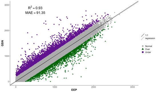
Figure 4.
Growing Season Normalized Difference Vegetation Index (GSN) regressed on Expected Ecosystem Performance (EEP) predicted from the EEP model with 1:1 line, regression line, and 90% confidence limits (normal, gray color) displayed. Over- (purple color) and underperformance (green color) points located outside of the 90% confidence limits represent the influence of non-climatic and site factors (e.g., overgrazing, fire, pests).
4.3. Conversion to Biomass
Annual EEP values serve as a proxy for forage production. The scatter plot of the annual EEP and SSURGO production shows a strong relation (R2 = 0.70) between these two variables (Figure 5). We observed some non-linear tendencies in the higher values of the EEP (EEP > 1500). Despite these, the linear fit between EEP and SSURGO productivity was found to be stronger than other non-linear fits (2nd degree polynomial and logarithmic). The observation density indicates that most observations fall along the regression line, while lower densities are associated with higher biomass values and points that are farther away from the regression line. This finding together with the increasing error rate (higher standard deviation for higher values) for higher biomass values might imply a lower predictability of biomass from EEP for high biomass areas. We observed a very strong relation (R2 = 0.99) between the cluster-averaged variables (Figure 5).
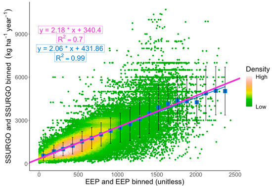
Figure 5.
Relation between Expected Ecosystem Performance (EEP) and Soil Survey Geographic Database (SSURGO) productivity across the study area and productivity categories. The scatter plot displays observation density where green points represent low density and red and white points represent high density of observations. The magenta elements (regression line, equation, and R2) represent the Weighted Least Squares (WLS) regression. The blue squares represent the mean of SSURGO values from bins of 20 clusters equally spaced along the range of the EEP values, and the blue elements represent regression of the binned values. The black error whiskers represent 2 standard deviations of the SSURGO values for each averaged cluster.
4.4. EB, Annual Biomass Deviation, and Percent Normal Biomass
EEP was converted to biomass and is displayed for two years as examples in Figure 6. Annual EB maps for the entire study period (2000–2018) can be found in Appendix B (Figure A2). These maps capture the spatial and temporal variability of biomass across the study area and years of analysis. The EB data are publicly available [64].
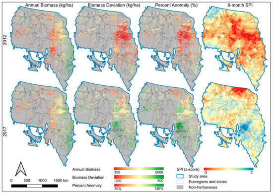
Figure 6.
Two example years (2012 and 2017) for annual expected biomass (kg ha−1), annual biomass deviation (kg ha−1), percent anomaly (%), and 6-month Standardized Precipitation Index (SPI) at the end of August in the study region.
Annual biomass deviation maps (Figure 6 and Figure A3) provide information of biomass departure from the long-term median value. Two example years of biomass deviation are presented in Figure 6, and all years (2000–2018) can be found in Appendix B (Figure A3). These maps show areas in specific years where biomass was lower or higher than normal.
The percent anomaly maps (Figure 6 and Figure A4), derived from the EB and long-term median EB, effectively show the spatial distribution of areas where the seasonal climate had a positive or a negative effect on biomass. Example percent anomaly maps from 2012 and 2017 are displayed in Figure 6. Maps for all years (2000–2018) can be found in Appendix B (Figure A4). In 2012, the biomass deviation map and the percent anomaly map showed low biomass production in the majority of the Great Plains region. On the other hand, in 2017, there was higher than normal biomass in the southern Great Plains and the Great Basin area, while a reduction was observed in the northern Great Plains. The areas of abnormally low and high production correspond to areas of drought and abnormally high precipitation as summarized for the period of the growing season (from the beginning of March through the end of August) using the SPI with a 6-month time-step (Figure 6).
4.5. Validation of the EEP Model
Comparison of the model-derived and the ground-observed biomass showed a moderately strong relation for the overall relation across time and space (Figure 7). Based on the regression analysis, the model explained 67% of the overall ground-observed variability.
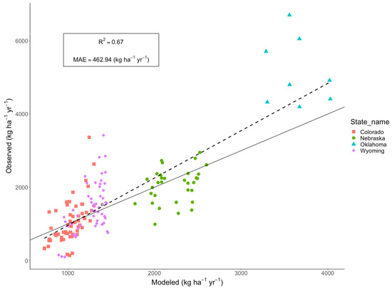
Figure 7.
Scatter plot of the ground-observed versus modeled annual biomass (kg ha−1). Different locations of data collection sites are distinguished by color and shape of points. Each point represents a year of observation. The solid black line represents the linear regression model fit, while the dashed line is a 1:1 line.
The time-series of modeled and observed biomass revealed that the model captured the variability in ground-observed biomass (Figure 8) across spatial and temporal dimensions. Underprediction of higher observed ground biomass was more pronounced for more sites in Colorado and Wyoming. The annual trend analysis revealed that the modeled data follow the same trend (decrease/increase) when compared to a previous year of production as the observed data in 75% of cases.
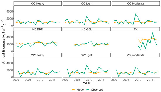
Figure 8.
Time-series analysis with subplots representing various validation sites located in the study area. The modeled annual biomass in kg ha−1 is displayed in yellow, while green represents the ground-observed data.
Time-series and regression analyses were performed separately for three validation sites near Cheyenne, Wyoming, to assess the model predictions beyond the time period of the model training database (Figure 9) using extrapolation of the model output using the historical climate data. The time-series plots (Figure 9A) capture the similarities and differences in the peaks and troughs between the modeled and ground-observed biomass, while the regression plots (Figure 9B) show the similarities of the model predictions, with respect to ground-observed data, in the training period and prior to it. The regression lines created for the historical and recent data (1982–1999 and 2001–2018, respectively) fell within the 90th confidence limits of the recent data regression (2001–2018).
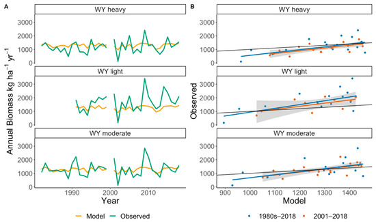
Figure 9.
Time-series (A) and regression (B) analyses of the observed versus modeled values of annual biomass for historical and present observations. In plot A, the modeled annual biomass in kg ha−1 is displayed in yellow, while the ground-observed biomass is green. In subplot B, the blue dots represent historical annual biomass values (from 1982 for Wyoming heavy and moderate and from 1991 for Wyoming light) until the year 1999. The orange points represent values from 2001 until 2018 (hereby recent). The blue line represents regression for historical and recent data, while the orange line with gray area of 95th confidence limits represent regression only for the recent data. The gray line represents a 1:1 relation.
5. Discussion and Conclusions
The remoteness of certain U.S. areas makes tracking changes and quantifying impacts of drought on vegetation difficult to monitor [51]. Our findings contribute to this effort by providing a landscape-scale understanding of forage dynamics across major U.S. semi-arid grasslands. For this area we developed an EEP model that estimates the amount of annual forage in a specific location based on seasonal and interannual climate variability, reducing the effect on non-climatic influences. The EEP was converted to biomass (kg ha−1 yr−1) and compared to ground-based biomass observations resulting in moderately strong relations. The maps of percent anomaly from a long-term median derived from the EEP model capture the effect of interannual climate variability on forage production with respect to a long-term production at a specific location. Because the regression lines created for the historical and recent data (Figure 9B) are sufficiently similar, we conclude that the model can be used for estimating forage production in years prior and after the model training period (2000–2018).
The ecosystem performance approach, used in this study, has been well established for the observation of ecosystem performance anomalies (difference between observed GSN and EEP) caused by fire, management, and other non-climatic factors [40,45,47,48,50]. Our study focused on the opposite process, using the EEP to capture the interannual variability of specific locations caused explicitly by changes in seasonal and interannual climate, while reducing the effect of non-climatic factors, a concept used by Poděbradská et al. [3]. Based on the model evaluation using the testing dataset we conclude that the model prediction was robust with a low degree of over- and underfitting, as well as minimal bias (Figure 4). The model under- and overperformances can be attributed mostly to non-climatic factors such as, fire, pest or disease infestation, land use and land cover changes, and management (e.g., overgrazing). Based on the model attribute usage, we found that the site potential is the most important factor when estimating grass biomass, which is consistent with findings of Wylie et al. [50]. The second most important factor is the accumulated summer precipitation in June, July, and August. These two variables were also found to be the most important in the Nebraska Sandhills, only in the opposite order (summer precipitation the most important, site potential the second most important) [3]. This result is expected because our model represents much larger growth potential variability than represented in the Nebraska Sandhills and therefore can capture more differences in annual biomass production across the area than the summer precipitation.
The site potential captures areas of higher and lower grass growth potential (Figure 2). The spatial patterns of growth potential are consistent with previous findings. For example, the site potential reflects a production gradient across the Great Plains from the more productive south-east region to the less productive north-west region [11], a similar gradient across the Greater Platte River Basin [48,65] and Nebraska Sandhills [3], and depicts similar patterns of growth potential across the Upper Colorado River Basin as found by Gu and Wylie [47].
The MAE of long-term GSN provides insight for areas with high and low interannual variability in forage production. We found an agreement with Reeves et al. [5] in certain locations of low (e.g., Flint Hills, Nebraska Sandhills, and north-central Wyoming) and high (e.g., central and western South Dakota and southern Texas) variability, while there were also differences in our findings (e.g., eastern Texas and eastern Wyoming). Based on the combined information from the site potential and MAE of long-term GSN, locations across the western United States can be categorized into four groups: (1) low growth potential with high interannual variability, (2) low growth potential with low interannual variability, (3) high growth potential with high interannual variability, and (4) high growth potential with low interannual variability. This information can be related to adaptive range management and flexible stocking. For example, areas characterized by low growth potential with high interannual variability (e.g., some areas in Utah, southeast Montana, and western Texas) might benefit from highly flexible livestock operations. On the other hand, areas that are highly productive and with low interannual variability (e.g., Flint Hills) may be able to manage their operations in a more conservative way without implementing highly flexible management strategies.
The results of conversion between unitless EEP and SSURGO show good relations for both the entire dataset and the binned values. The observed noise in this relation can be mostly attributed to the characteristics of the SSURGO dataset. The values of biomass production in SSURGO are determined based on ground observations and further assigned to areas that have the same biophysical properties (e.g., soil associations). This sometimes leads to large areas having the exact same biomass production values, which is unrealistic. Similar results were found by Gu et al. [65] for the Greater Platte River Basin. Gu et al. [65] used a slightly different method for representing the GSN and used only the representative SSURGO values depicting a “normal year” for precipitation and forage production. We observed a non-linear relation between EEP and SSURGO for higher EEP values, due to an underestimation of ecosystem productivity in dense vegetation canopies as found by previous studies [66,67].
We used the time-integrated NDVI as a proxy for annual forage production because it has been widely used both for biomass estimation and in EEP models. However, some studies observed better relations between biomass and other remotely sensed biomass proxies, for example, the Absorbed Photosynthetically Active Radiation (APAR, [68]). Future research could investigate the use of these or other vegetation indices such as the leaf area index, enhanced vegetation index, and APAR in EEP models.
The EB maps captured the wet and dry years as well as the variability in growth potential across the study area (Figure 6 and Figure A2). The maps of annual biomass deviation (Figure 6 and Figure A3) depict the biomass departure from the long-term median, which reflects the effect of seasonal and interannual climate conditions on biomass production. Maps of percent anomaly (Figure 6 and Figure A4) depict the percent departure from the long-term median biomass, which captures the effect of seasonal and interannual climate conditions on biomass production with respect to production at a specific location. These maps are the most intuitive for depicting the below and above normal biomass conditions in different years caused by intra- and interannual climate variability and can be connected to the four groups of site potential and long-term MAE. For example, during the drought year 2012, the biomass in the Flint Hills (eastern Kansas) was around 3500 kg ha−1. The biomass deviation maps show a negative departure between 250 and 500 kg ha−1, which is depicted as two of the most severe negative categories, but the percent anomaly maps revealed only a 10–20% departure. The Flint Hills are in a category of high site potential and low interannual variability. On the other hand, low-productive areas in northern Utah showed a slight negative biomass deviation (~−150 kg ha−1) while also having a high negative percent anomaly (less than 70% of normal). This is also observed for positive biomass deviations and percent anomalies (e.g., as observed in the same Utah area in 2017, Figure 6). If these maps were provided as predictions during the growing season, livestock producers and land managers would be able to see where the major positive and negative departures from normal are expected to occur, which they could use as a basis for their decision-making (e.g., where to relocate cattle or buy additional feed).
To validate our EEP model together with the conversion to biomass using SSURGO data, we compared the modeled biomass data with long-term grass clipping data from various locations in the study area. The R2 value of the observed versus modeled biomass indicated a moderately strong relation and was comparable to values observed in other studies [3,26,69]. The ground-observed clipping data were in most cases obtained from multiple small rectangles (0.25-m2) and scaled to the entire pasture, while the modeled data captured much larger areas (62,500-m2) averaged over a few pixels covering the entire pasture. Both techniques can introduce errors that can result in lower R2 values. In most cases the ground observations were obtained from small areas that were not grazed during the current season, while the modeled data that are based on satellite observations capture a signal from the entire pasture that was under a certain grazing pressure. This can partially explain the bias in the observed versus modeled data. Additional errors could also have been introduced during the conversion of the EEP values to biomass using the SSURGO database. This database is known to contain state and county discontinuities that are caused by differences in survey methods over decades of soil data collection; however, there are emerging techniques that address this issue (e.g., the POLARIS soil series map, [70]). The time-series validation plots reveal that the model reasonably predicts the trend in biomass amount. However, overestimation of very low and underestimation of very high ground-observed biomass can be observed. The time-series and regression analysis on the extended historical data from the Cheyenne, Wyoming, area indicate that the model can be used beyond its training period, creating opportunities for analysis of temporal trends of forage production in the past and future.
Using this modelling method, we established a relation between biomass production and seasonal climate for western U.S. semi-arid grasslands. This relation can be utilized for creating historical and future biomass estimates without the use of remotely sensed data. This is especially valuable for time periods when remote sensing data are not available, for example, before the Landsat era starting in 1972 or for future climate change scenarios. However, these estimates warrant interpretation with caution as some important local characteristics such as species composition and land use can change over longer time periods. Additionally, the older historical gridded climate data are created from a smaller number of weather stations leading to more extrapolation between the observed data and to potential errors in the climate data, an input of the forage model. The model can also be used for early predictions of annual biomass together with seasonal climate forecasts and scenarios to support within-season decision-making of livestock producers and land managers.
Future research could focus on comparison of the annual biomass estimates in this study with other similar approaches like the Rangeland Production Monitoring Service, Rangeland Analysis Platform, and Grass-Cast end-of-season estimates. Grassland biomass growth is affected by many complex processes that occur on the stand level. Further research could be helpful to understand the effect of hot dry summer conditions on the grass dormancy. A better understanding and effective large scale monitoring of the geographic distribution of warm and cool season grasses can help better explain the dynamics of forage production in the future. Because grasslands are not the only component of rangelands, which also include shrublands and savannas, exploring application of this methodology to other rangeland land covers is desirable. The method introduced in this manuscript can be used with global NDVI and climate datasets to develop estimates of forage biomass across global grassland areas. Finally, higher spatial resolution (e.g., 30-m) would lead to an improvement in capturing the within-pasture variability in forage production and would be more relevant for individual livestock operations and from the perspective of fire fuel load modeling. Newly emerging data fusion techniques (e.g., fusion of NDVI observations from Landsat and Sentinel-2) can leverage this type of spatial resolution with high observation frequency, which is important for characterization of growing season phenology [71] and precise estimates of the growing season NDVI [72]. Future efforts could explore the use of these or similar NDVI datasets in the forage production model. However, it is important to note that other datasets used in the forage production model would need to match the spatial resolution of the NDVI data. This is problematic especially for temperature and precipitation data, which are usually produced with a coarser spatial resolution (e.g., 1-km).
Author Contributions
Conceptualization, M.P., B.K.W., M.J.H., B.D.W., D.J.B.; methodology, M.P., B.K.W., M.J.H., B.D.W., D.J.B.; software, B.K.W., D.D., M.P.; validation, M.P., J.D.D., P.A.F., W.H.S., J.D.V., P.W.; formal analysis, M.P., Y.A.B.; investigation, M.P., Y.A.B.; resources, B.K.W., D.D.; data curation, M.P., B.K.W., D.D.; writing—original draft preparation, M.P.; writing—review and editing, M.P., B.K.W., M.J.H., B.D.W., D.J.B., Y.A.B., J.D.D., P.A.F., W.H.S., J.D.V., P.W.; visualization, M.P.; supervision, B.K.W., M.J.H., B.D.W., D.J.B.; project administration, M.J.H., B.K.W.; funding acquisition, M.J.H., M.P., B.D.W., B.K.W. All authors have read and agreed to the published version of the manuscript.
Funding
This research was funded by the U.S. Geological Survey Land Change Science Program through U.S. Geological Survey Cooperative Agreement No. G19AC00074 and G20AC00398. Final analyses and review performed by M.P. were supported by the SustES project—adaptation strategies for sustainable ecosystem services and food security under adverse environmental conditions (CZ.02.1.01/0.0/0.0/16_019/0000797).
Institutional Review Board Statement
Not applicable.
Informed Consent Statement
Not applicable.
Data Availability Statement
The data are publicly available at https://doi.org/10.5066/P98HOCL6 (last accessed on 18 November 2021).
Acknowledgments
The authors would like to thank Matthew Rigge from the U.S. Geological Survey for his review of the manuscript and his valuable comments and revisions. We would like to thank all the anonymous reviewers for their valuable comments and helpful suggestions, which lead to substantial improvements in the manuscript. Any use of trade, firm, or product names is for descriptive purposes only and does not imply endorsement by the U.S. Government.
Conflicts of Interest
The authors declare no conflict of interest.
Appendix A. Delineation of Model Training Areas and Placement of Training Points
The selection of training points (pixels), their location, distribution, and number are important factors for developing a Regression Tree (RT) model that aims to be representative of the entire study area and the modeled Land Cover (LC) class. Our study focused only on grassland LC. To limit an effect of mixed pixels (signal coming from multiple LC classes) in the model training database, we used LC data with higher spatial resolution (30-m, National Land Cover Database 2016 (NLCD 2016)) to identify 250-m pixels (resolution of the model input data) that contained a high percentage of herbaceous cover. The signal can therefore be attributed mostly to herbaceous LC. Specifically, we used the NLCD (available on www.mrlc.gov) in multiple epochs (2001, 2003, 2006, 2008, 2011, 2013, and 2016) and the National Gap Analysis Project Land Cover mapping (available on https://www.usgs.gov/core-science-systems/science-analytics-and-synthesis/gap, last accessed on 18 November 2021) for identification of 30-m LC categories. Irrigated land (from Moderate Resolution Imaging Spectroradiometer (MODIS) Irrigated Agriculture available on https://www.usgs.gov/special-topics/monitoring-vegetation-drought-stress/science/modis-irrigated-agriculture (last accessed on 18 November 2021) was excluded from the suitable training areas, because the relation between vegetation condition and climate can be altered by application of irrigation water. Areas with a high percentage of annual cheatgrass cover (https://rangelands.app/cheatgrass/, last accessed on 18 November 2021) were excluded from training and mapped areas due to difference in seasonality compared to perennial vegetation [73]. Areas with a high amount of elevation variation (from The National Map available on https://nationalmap.gov/elevation.html, last accessed on 18 November 2021) can experience high variability in precipitation and temperature over small linear distances [74] and therefore were excluded due to uncertainties connected to the climate data downscaling process. Finally, alpine tundra (data from the National GAP Land Cover mapping) was excluded from the training and mapped areas due to frequent snow cover and lower responsiveness to the variability in precipitation [51]. The remaining pixels were identified as suitable for our model training database. Table A1 summarizes the criteria based on which pixels were considered suitable for placement of training points and criteria used for displaying the model results (mapped areas), which use slightly less restrictive criteria. The criteria were more restrictive for Region A (Figure 1), which has more continuous herbaceous cover, than Region B, which is characterized by high occurrence of shrubland LC with scattered herbaceous areas.

Table A1.
Summary of conditions for selecting representative pixels for the model training database and for identifying areas that can be displayed as herbaceous using our model output. The percent herbaceous, water, wetlands, and cheatgrass are relevant for each 250-m pixel of the study site.
Table A1.
Summary of conditions for selecting representative pixels for the model training database and for identifying areas that can be displayed as herbaceous using our model output. The percent herbaceous, water, wetlands, and cheatgrass are relevant for each 250-m pixel of the study site.
| Criteria | Regions | Percent Herbaceous Cover | Percent Water and Wetlands | Percent Cheatgrass Cover | Number of Years Classified as Grassland in NLCD Epochs | Elevation Variation |
|---|---|---|---|---|---|---|
| Training areas | Region A | 100 | 0 | N/A | 7 out of 7 | Standard deviation of elevation in the surrounding 4-km area < 150 m |
| Region B | 80 | 20 | 5 out of 7 | |||
| Mapped areas | Region A | 90 | 10 | N/A | Correspond to the closest NLCD mapping year | Not considered |
| Region B | 75 | 15 |
The suitable training areas determined pixels where the model database training points could be placed. The number of points used for the model training database was based on the number of points from Poděbradská et al. [3] and scaled to the total mapped area (n = 347,414). The placement of the training points should be stratified across space, time, and forage production gradient. The number of training points placed in each Omernik Level III ecoregion (L3E, [75]) was determined based on a logarithmically weighted proportion of the mapped area within each ecoregion compared to a total mapped area. This ensured an inclusion of training points from areas with both high and low density of herbaceous cover. To represent a range of possible annual forage production, the GSN in every L3E was divided into 6 groups for every year of our analysis (2000–2018). One-sixth of the training points for each L3E was then randomly placed into the suitable training areas of each productivity category for each year. This ensured that both extremely low and high productivity values are represented equally in the model and theoretically lead to a better estimation of extreme values as recommended by Poděbradská et al. [3].
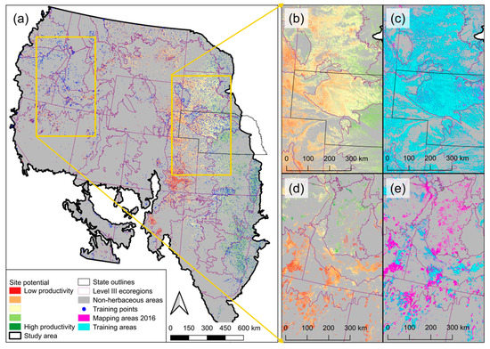
Figure A1.
The study area with site potential values and the distribution of model training points for one year of the study period (a). Maps (b,d) depict the site potential for the central Great Plains and the northwest part of the study area, respectively. Maps (c,e) show the difference between pixels identified as suitable for training point placement and the areas for which our results were displayed in year 2016.

The total unmasked study area was over 3 million km2, while the area considered for displaying results was around 550 thousand km2 or about 17 percent of the entire study area. The area used for placement of model database training points was considerably smaller, around 400 thousand km2 or 12.5 percent of the entire study area. Larger differences in mapped and training areas were observed for the western part of the study region (Region B) due to the smaller size of grassland patches and intermixed shrubland components. An example of these differences is provided in Appendix A (Figure A1).
Appendix B
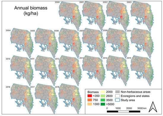
Figure A2.
Maps of annual expected biomass in kg ha−1 as predicted by the Expected Ecosystem Performance (EEP) model (2000–2018). Lower biomass is displayed in red and high biomass in green colors.
Figure A2.
Maps of annual expected biomass in kg ha−1 as predicted by the Expected Ecosystem Performance (EEP) model (2000–2018). Lower biomass is displayed in red and high biomass in green colors.

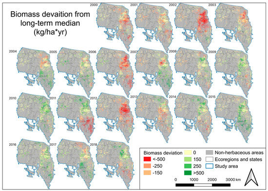
Figure A3.
Maps of annual biomass deviation (2000–2018) from a long-term median value in kg ha−1. Large negative departures are displayed in red, while large positive departures from median in green color.
Figure A3.
Maps of annual biomass deviation (2000–2018) from a long-term median value in kg ha−1. Large negative departures are displayed in red, while large positive departures from median in green color.

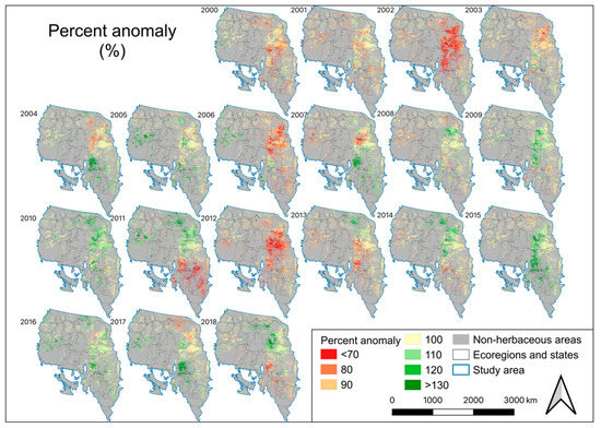
Figure A4.
Maps of percent anomaly (2000–2018) from long-term median value (which equals 100%). Red values capture location-specific negative departures and represent lower than normal biomass.
Figure A4.
Maps of percent anomaly (2000–2018) from long-term median value (which equals 100%). Red values capture location-specific negative departures and represent lower than normal biomass.

References
- USDA NRCS Rangelands. Available online: https://www.nrcs.usda.gov/wps/portal/nrcs/detailfull/national/landuse/rangepasture/range/?cid=STELPRDB1043345 (accessed on 1 July 2021).
- Derner, J.; Briske, D.; Reeves, M.; Brown-Brandl, T.; Meehan, M.; Blumenthal, D.; Travis, W.; Augustine, D.; Wilmer, H.; Scasta, D.; et al. Vulnerability of grazing and confined livestock in the Northern Great Plains to projected mid- and late-twenty-first century climate. Clim. Chang. 2018, 146, 19–32. [Google Scholar] [CrossRef]
- Poděbradská, M.; Wylie, B.K.; Hayes, M.J.; Wardlow, B.D.; Bathke, D.J.; Bliss, N.B.; Dahal, D. Monitoring drought impact on annual forage production in semi-arid grasslands: A case study of Nebraska sandhills. Remote Sens. 2019, 11, 2106. [Google Scholar] [CrossRef] [Green Version]
- Reeves, M.C.; Bagne, K.E. Vulnerability of Cattle Production to Climate Change on U.S. Rangelands; US Department of Agriculture, Forest Service: Fort Collins, CO, USA, 2016; 39p.
- Reeves, M.C.; Hanberry, B.B.; Wilmer, H.; Kaplan, N.E.; Lauenroth, W.K. An Assessment of Production Trends on the Great Plains from 1984 to 2017. Rangel. Ecol. Manag. 2021, 78, 165–179. [Google Scholar] [CrossRef]
- Stanke, C.; Kerac, M.; Prudhomme, C.; Medlock, J.; Murray, V. Health effects of drought: A systematic review of the evidence. PLoS Curr. 2013, 5. [Google Scholar] [CrossRef] [Green Version]
- Knutson, C.L.; Haigh, T.R. Ranchers in the United States, scientific information, and drought risk. In Drought, Risk Management, and Policy: Decision-Making under Uncertainty; Botterill, L.C., Cockfield, G., Eds.; CRC Press: Boca Raton, FL, USA, 2013; p. 171. [Google Scholar]
- Rippey, B. Agricultural Weather and Drought Update—8/21/12. Available online: https://www.usda.gov/media/blog/2012/08/21/agricultural-weather-and-drought-update-82112 (accessed on 19 August 2020).
- Rippey, B.U.S. Drought Monitor and USDA Financial Assistance Programs. Available online: http://beef.okstate.edu/files/usdm-and-usda-financial-assistance-programs (accessed on 28 May 2021).
- Leister, A.M.; Paarlberg, P.L.; Lee, J.G. Dynamic effects of drought on US crop and livestock sectors. J. Agric. Appl. Econ. 2015, 47, 261–284. [Google Scholar] [CrossRef] [Green Version]
- Sala, O.E.; Parton, W.J.; Joyce, L.A.; Lauenroth, W.K. Primary production of the central grassland region of the United States. Ecology 1988, 69, 40–45. [Google Scholar] [CrossRef]
- Knapp, A.K.; Smith, M.D. Variation among biomes in temporal dynamics of aboveground primary production. Science 2001, 291, 481–484. [Google Scholar] [CrossRef] [Green Version]
- Derner, J.D.; Hart, R.H. Grazing-induced modifications to peak standing crop in northern mixed-grass prairie. Rangel. Ecol. Manag. 2007, 60, 270–276. [Google Scholar] [CrossRef]
- Derner, J.D.; Augustine, D.J.; Briske, D.D.; Wilmer, H.; Porensky, L.M.; Fernández-Giménez, M.E.; Peck, D.E.; Ritten, J.P. Can Collaborative Adaptive Management Improve Cattle Production in Multipaddock Grazing Systems? Rangel. Ecol. Manag. 2021, 75, 1–8. [Google Scholar] [CrossRef]
- Bement, R.E. A stocking-rate guide for beef production on blue-grama range. Rangel. Ecol. Manag. Range Manag. Arch. 1969, 22, 83–86. [Google Scholar] [CrossRef] [Green Version]
- Raynor, E.J.; Derner, J.D.; Baldwin, T.; Ritten, J.P.; Augustine, D.J. Multidecadal directional shift in shortgrass stocking rates. Rangel. Ecol. Manag. 2021, 74, 72–80. [Google Scholar] [CrossRef]
- Ritten, J.P.; Frasier, W.M.; Bastian, C.T.; Gray, S.T. Optimal rangeland stocking decisions under stochastic and climate-impacted weather. Am. J. Agric. Econ. 2010, 92, 1242–1255. [Google Scholar] [CrossRef]
- Peck, D.; Derner, J.; Parton, W.; Hartman, M.; Fuchs, B. Flexible stocking with Grass-Cast: A new grassland productivity forecast to translate climate outlooks for ranchers. West. Econ. Forum 2019, 17, 24–39. [Google Scholar]
- Derner, J.D.; Augustine, D.J. Adaptive Management for Drought on Rangelands. Rangelands 2016, 38, 211–215. [Google Scholar] [CrossRef] [Green Version]
- Bastian, C.T.; Ritten, J.P.; Derner, J.D. Ranch Profitability Given Increased Precipitation Variability and Flexible Stocking. J. ASFMRA 2018, 122–139. [Google Scholar] [CrossRef]
- Cheng, G.; Harmel, R.D.; Ma, L.; Derner, J.D.; Augustine, D.J.; Bartling, P.N.S.; Fang, Q.X.; Williams, J.R.; Zilverberg, C.J.; Boone, R.B.; et al. Evaluation of APEX modifications to simulate forage production for grazing management decision-support in the Western US Great Plains. Agric. Syst. 2021, 191, 103139. [Google Scholar] [CrossRef]
- Ma, L.; Derner, J.D.; Harmel, R.D.; Tatarko, J.; Moore, A.D.; Rotz, C.A.; Augustine, D.J.; Boone, R.B.; Coughenour, M.B.; Beukes, P.C.; et al. Application of grazing land models in ecosystem management: Current status and next frontiers. Adv. Agron. 2019, 158, 173–215. [Google Scholar] [CrossRef]
- Baumann, M.; Ozdogan, M.; Richardson, A.D.; Radeloff, V.C. Phenology from Landsat when data is scarce: Using MODIS and Dynamic Time-Warping to combine multi-year Landsat imagery to derive annual phenology curves. Int. J. Appl. Earth Obs. Geoinf. 2017, 54, 72–83. [Google Scholar] [CrossRef]
- Zhu, Z.; Woodcock, C.E.; Holden, C.; Yang, Z. Generating synthetic Landsat images based on all available Landsat data: Predicting Landsat surface reflectance at any given time. Remote Sens. Environ. 2015, 162, 67–83. [Google Scholar] [CrossRef]
- Jones, M.O.; Robinson, N.P.; Naugle, D.E.; Maestas, J.D.; Reeves, M.C.; Lankston, R.W.; Allred, B.W. Annual and 16-day rangeland production estimates for the western united states. bioRxiv 2020. [Google Scholar] [CrossRef]
- Hartman, M.D.; Parton, W.J.; Derner, J.D.; Schulte, D.K.; Smith, W.K.; Peck, D.E.; Day, K.A.; Del Grosso, S.J.; Lutz, S.; Fuchs, B.A.; et al. Seasonal grassland productivity forecast for the U.S. Great Plains using Grass-Cast. Ecosphere 2020, 11, e03280. [Google Scholar] [CrossRef]
- Kriegler, F.J.; Malila, W.A.; Nalepka, R.F.; Richardson, W. Preprocessing transformations and their effects on multispectral recognition. Remote Sens. Environ. 1969, VI, 97–132. [Google Scholar]
- AghaKouchak, A.; Farahmand, A.; Melton, F.S.; Teixeira, J.; Anderson, M.C.; Wardlow, B.D.; Hain, C.R. Remote sensing of drought: Progress, challenges and opportunities. Rev. Geophys. 2015, 53, 452–480. [Google Scholar] [CrossRef] [Green Version]
- Ji, L.; Wylie, B.K.; Nossov, D.R.; Peterson, B.; Waldrop, M.P.; McFarland, J.W.; Rover, J.; Hollingsworth, T.N. Estimating aboveground biomass in interior Alaska with Landsat data and field measurements. Int. J. Appl. Earth Obs. Geoinf. 2012, 18, 451–461. [Google Scholar] [CrossRef]
- Wylie, B.K.; Meyer, D.J.; Tieszen, L.L.; Mannel, S. Satellite mapping of surface biophysical parameters at the biome scale over the North American grasslands a case study. Remote Sens. Environ. 2002, 79, 266–278. [Google Scholar] [CrossRef]
- Heim, R.R. A review of twentieth-century drought indices used in the United States. Bull. Am. Meteorol. Soc. 2002, 83, 1149–1165. [Google Scholar] [CrossRef] [Green Version]
- White, A.B.; Kumar, P.; Tcheng, D. A data mining approach for understanding topographic control on climate-induced inter-annual vegetation variability over the United States. Remote Sens. Environ. 2005, 98, 1–20. [Google Scholar] [CrossRef]
- Stephenson, M.B.; Volesky, J.D.; Schacht, W.H.; Lawrence, N.C.; Soper, J.; Milby, J. Influence of Precipitation on Plant Production at Different Topographic Positions in the Nebraska Sandhills. Rangel. Ecol. Manag. 2019, 72, 103–111. [Google Scholar] [CrossRef]
- Lauenroth, W.K.; Sala, O.E. Long-term forage production of North American shortgrass steppe. Ecol. Appl. 1992, 2, 397–403. [Google Scholar] [CrossRef] [PubMed] [Green Version]
- Bradford, J.B.; Lauenroth, W.K.; Burke, I.C.; Paruelo, J.M. The influence of climate, soils, weather, and land use on primary production and biomass seasonality in the US Great Plains. Ecosystems 2006, 9, 934–950. [Google Scholar] [CrossRef]
- Snyman, H.A. Short-term response in productivity following an unplanned fire in a semi-arid rangeland of South Africa. J. Arid Environ. 2004, 56, 465–485. [Google Scholar] [CrossRef]
- Zydenbos, S.M.; Barratt, B.I.P.; Bell, N.L.; Ferguson, C.M.; Gerard, P.J.; Mcneill, M.R.; Phillips, C.B.; Townsend, R.J.; Jackson, T.A. The impact of invertebrate pests on pasture persistence and their interrelationship with biotic and abiotic factors. NZGA Res. Pract. Ser. 2011, 15, 109–117. [Google Scholar] [CrossRef]
- Moran, M.S.; Ponce-Campos, G.E.; Huete, A.; McClaran, M.P.; Zhang, Y.; Hamerlynck, E.P.; Augustine, D.J.; Gunter, S.A.; Kitchen, S.G.; Peters, D.P.C.; et al. Functional response of U.S. grasslands to the early 21st-century drought. Ecology 2014, 95, 2121–2133. [Google Scholar] [CrossRef]
- Petrie, M.D.; Peters, D.P.C.; Yao, J.; Blair, J.M.; Burruss, N.D.; Collins, S.L.; Derner, J.D.; Gherardi, L.A.; Hendrickson, J.R.; Sala, O.E.; et al. Regional grassland productivity responses to precipitation during multiyear above-and below-average rainfall periods. Glob. Chang. Biol. 2018, 24, 1935–1951. [Google Scholar] [CrossRef]
- Wylie, B.; Zhang, L.; Bliss, N.; Ji, L.; Tieszen, L.L.; Jolly, W.M. Integrating modelling and remote sensing to identify ecosystem performance anomalies in the boreal forest, Yukon River Basin, Alaska. Int. J. Digit. Earth 2008, 1, 196–220. [Google Scholar] [CrossRef]
- Omernik, J.M. Ecoregions: A framework for managing ecosystems. Georg. Wright Forum 1995, 12, 35–50. [Google Scholar]
- Sala, O.E.; Paruelo, J.M. Ecosystem Services in Grasslands. In Nature’s Services: Societal Dependence on Natural Ecosystems; Daily, G.C., Ed.; Island Press: Washington, DC, USA, 1997; pp. 237–251. [Google Scholar]
- Hayhoe, K.; Wuebbles, D.J.; Easterling, D.R.; Fahey, D.W.; Doherty, S.; Kossin, J.; Sweet, W.; Vose, R.; Wehner, M. Our Changing Climate. In Impacts, Risks, and Adaptation in the United States: Fourth National Climate Assessment; Reidmiller, D.R., Avery, C.W., Easterling, D.R., Kunkel, K.E., Lewis, K.L.M., Maycock, T.K., Stewart, B.C., Eds.; U.S. Global Change Research Program: Washington, DC, USA, 2018; Volume II. [Google Scholar]
- Quinlan, J.R. Learning with continuous classes. In Proceedings of the 5th Australian joint conference on artificial intelligence, Hobart, Australia, 16–18 November 1992; pp. 343–348. [Google Scholar]
- Boyte, S.P.; Wylie, B.K.; Major, D.J. Mapping and monitoring cheatgrass dieoff in rangelands of the Northern Great Basin, USA. Rangel. Ecol. Manag. Manag. 2015, 68, 18–28. [Google Scholar] [CrossRef]
- Boyte, S.P.; Wylie, B.K.; Gu, Y.; Major, D.J. Estimating Abiotic Thresholds for Sagebrush Condition Class in the Western United States. Rangel. Ecol. Manag. 2020, 73, 297–308. [Google Scholar] [CrossRef]
- Gu, Y.; Wylie, B.K. Detecting ecosystem performance anomalies for land management in the Upper Colorado River Basin using satellite observations, climate data, and ecosystem models. Remote Sens. 2010, 2, 1880–1891. [Google Scholar] [CrossRef] [Green Version]
- Rigge, M.; Wylie, B.; Gu, Y.; Belnap, J.; Phuyal, K.; Tieszen, L. Monitoring the status of forests and rangelands in the Western United States using ecosystem performance anomalies. Int. J. Remote Sens. 2013, 34, 4049–4068. [Google Scholar] [CrossRef]
- RuleQuest Research Cubist; Version 2.07; RuleQuest Research Pty Ltd.: St Ives, NSW, Australia, 2008.
- Wylie, B.K.; Boyte, S.P.; Major, D.J. Ecosystem performance monitoring of rangelands by integrating modeling and remote sensing. Rangel. Ecol. Manag. 2012, 65, 241–252. [Google Scholar] [CrossRef]
- El-Vilaly, M.A.S.; Didan, K.; Marsh, S.E.; van Leeuwen, W.J.D.; Crimmins, M.A.; Munoz, A.B. Vegetation productivity responses to drought on tribal lands in the four corners region of the Southwest USA. Front. Earth Sci. 2018, 12, 37–51. [Google Scholar] [CrossRef]
- Tieszen, L.L.; Reed, B.C.; Bliss, N.B.; Wylie, B.K.; DeJong, D.D. NDVI, C3 and C4 production, and distributions in Great Plains grassland land cover classes. Ecol. Appl. 1997, 7, 58–78. [Google Scholar] [CrossRef]
- Yang, L.; Wylie, B.K.; Tieszen, L.L.; Reed, B.C. An analysis of relationships among climate forcing and time-integrated NDVI of grasslands over the U.S. northern and central Great Plains. Remote Sens. Environ. 1998, 65, 25–37. [Google Scholar] [CrossRef]
- Jenkerson, C.; Maiersperger, T.; Schmidt, G. eMODIS: A User-Friendly Data Source; USGS: Denver, CO, USA, 2010.
- Swets, D.L.; Reed, B.C.; Rowland, J.D.; Marko, S.E. A weighted least-squares approach to temporal smoothing of NDVI. In Proceedings of the ASPRS Annual Conference, From Image to Information; American Society for Photogrammetry and Remote Sensing, Bethesda: Portland, OR, USA, 1999. [Google Scholar]
- Montandon, L.M.; Small, E.E. The impact of soil reflectance on the quantification of the green vegetation fraction from NDVI. Remote Sens. Environ. 2008, 112, 1835–1845. [Google Scholar] [CrossRef]
- PRISM Climate Group PRISM Climate Group. Available online: http://prism.oregonstate.edu/ (accessed on 10 October 2020).
- Pastick, N.J.; Wylie, B.K.; Rigge, M.B.; Dahal, D.; Boyte, S.P.; Jones, M.O.; Allred, B.W.; Parajuli, S.; Wu, Z. Rapid Monitoring of the Abundance and Spread of Exotic Annual Grasses in the Western United States Using Remote Sensing and Machine Learning. AGU Adv. 2021, 2, e2020AV000298. [Google Scholar] [CrossRef]
- Gu, Y.; Wylie, B.K.; Boyte, S.P.; Picotte, J.; Howard, D.M.; Smith, K.; Nelson, K.J. An optimal sample data usage strategy to minimize overfitting and underfitting effects in regression tree models based on remotely-sensed data. Remote Sens. 2016, 8, 943. [Google Scholar] [CrossRef] [Green Version]
- McKee, T.B.; Doesken, N.J.; Kleist, J. The relationship of drought frequency and duration to time scales. In Proceedings of the Eighth Conference on Applied Climatology, Anaheim, CA, USA, 17–22 January 1993. [Google Scholar]
- Irisarri, J.G.N.; Derner, J.D.; Porensky, L.M.; Augustine, D.J.; Reeves, J.L.; Mueller, K.E. Grazing intensity differentially regulates ANPP response to precipitation in North American semiarid grasslands. Ecol. Appl. 2016, 26, 1370–1380. [Google Scholar] [CrossRef] [Green Version]
- Wagle, P.; Gowda, P.H.; Northup, B.K.; Starks, P.J.; Neel, J.P.S. Response of tallgrass prairie to management in the U.S. Southern great plains: Site descriptions, management practices, and eddy covariance instrumentation for a Long-Term Experiment. Remote Sens. 2019, 11, 1988. [Google Scholar] [CrossRef] [Green Version]
- RuleQuest Research An Overview of Cubist. Available online: https://www.rulequest.com/cubist-win.html#CTTEE (accessed on 28 May 2021).
- Poděbradská, M.; Wylie, B.K.; Dahal, D. Time Series of Expected Livestock Forage Biomass in the Semi-Arid Grasslands of the Western U.S. (2000–2018); U.S. Geological Survey Data Release: Reston, VA, USA, 2021. [CrossRef]
- Gu, Y.; Wylie, B.K.; Bliss, N.B. Mapping grassland productivity with 250-m eMODIS NDVI and SSURGO database over the Greater Platte River Basin, USA. Ecol. Indic. 2013, 24, 31–36. [Google Scholar] [CrossRef]
- Asrar, G.Q.; Fuchs, M.; Kanemasu, E.T.; Hatfield, J.L. Estimating absorbed photosynthetic radiation and leaf area index from spectral reflectance in wheat 1. Agron. J. 1984, 76, 300–306. [Google Scholar] [CrossRef]
- Chen, P.-Y.; Fedosejevs, G.; Tiscareno-Lopez, M.; Arnold, J.G. Assessment of MODIS-EVI, MODIS-NDVI and VEGETATION-NDVI composite data using agricultural measurements: An example at corn fields in western Mexico. Environ. Monit. Assess. 2006, 119, 69–82. [Google Scholar] [CrossRef] [PubMed]
- Gaffney, R.; Porensky, L.M.; Gao, F.; Irisarri, J.G.; Durante, M.; Derner, J.D.; Augustine, D.J. Using APAR to predict aboveground plant productivity in semi-aid rangelands: Spatial and temporal relationships differ. Remote Sens. 2018, 10, 1474. [Google Scholar] [CrossRef] [Green Version]
- Wylie, B.K.; DeJong, D.D.; Tieszen, L.L.; Biondini, M.E. Grassland canopy parameters and their relationships to remotely sensed vegetation indices in the nebraska sand hills. Geocarto Int. 1996, 11, 39–52. [Google Scholar] [CrossRef]
- Chaney, N.W.; Wood, E.F.; McBratney, A.B.; Hempel, J.W.; Nauman, T.W.; Brungard, C.W.; Odgers, N.P. POLARIS: A 30-m probabilistic soil series map of the contiguous United States. Geoderma 2016, 274, 54–67. [Google Scholar] [CrossRef] [Green Version]
- Pastick, N.J.; Dahal, D.; Wylie, B.K.; Parajuli, S.; Boyte, S.P.; Wu, Z. Characterizing land surface phenology and exotic annual grasses in dryland ecosystems using landsat and sentinel-2 data in harmony. Remote Sens. 2020, 12, 725. [Google Scholar] [CrossRef] [Green Version]
- Pastick, N.J.; Wylie, B.K.; Wu, Z. Spatiotemporal analysis of Landsat-8 and Sentinel-2 data to support monitoring of dryland ecosystems. Remote Sens. 2018, 10, 791. [Google Scholar] [CrossRef] [Green Version]
- Boyte, S.P.; Wylie, B.K.; Major, D.J. Cheatgrass percent cover change: Comparing recent estimates to climate change—Driven predictions in the Northern Great Basin. Rangel. Ecol. Manag. 2016, 69, 265–279. [Google Scholar] [CrossRef]
- Barry, R.G. Mountain Weather and Climate; Psychology Press: Hove, UK, 1992. [Google Scholar]
- Omernik, J.M. Ecoregions of the Conterminous United States. Ann. Assoc. Am. Geogr. 1987, 77, 118–125. [Google Scholar] [CrossRef]
Publisher’s Note: MDPI stays neutral with regard to jurisdictional claims in published maps and institutional affiliations. |
© 2021 by the authors. Licensee MDPI, Basel, Switzerland. This article is an open access article distributed under the terms and conditions of the Creative Commons Attribution (CC BY) license (https://creativecommons.org/licenses/by/4.0/).


