Assessment of the Performance of TROPOMI NO₂ and SO₂ Data Products in the North China Plain: Comparison, Correction and Application

Abstract

The TROPOspheric Monitoring Instrument (TROPOMI) aboard the Sentinel-5 Precursor satellite has been used to detect the atmospheric environment since 2017, and it is of great significance to investigate the accuracy of its products. In this work, we present comparisons between TROPOMI tropospheric NO₂ and total SO₂ products against ground-based MAX-DOAS at a single site (Xianghe) and OMI products over a seriously polluted region (North China Plain, NCP) in China. The results show that both NO₂ and SO₂ data from three datasets exhibit a similar tendency and seasonality. In addition, TROPOMI tropospheric NO₂ columns are generally underestimated compared with collocated MAX-DOAS and OMI data by about 30–60%. In contrast to NO₂, the monthly average SO₂ retrieved from TROPOMI is larger than MAX-DOAS and OMI, with a mean bias of 2.41 (153.8%) and 2.17 × 10¹⁶ molec cm⁻² (120.7%), respectively. All the results demonstrated that the TROPOMI NO₂ as well as the SO₂ algorithms need to be further improved. Thus, to ensure reliable analysis in NCP area, a correction method has been proposed and applied to TROPOMI Level 3 data. The revised datasets agree reasonably well with OMI observations (R > 0.95 for NO₂, and R > 0.85 for SO₂) over the NCP region and have smaller mean biases with MAX-DOAS. In the application during COVID-19 pandemic, it showed that the NO₂ column in January-April 2020 decreased by almost 25–45% compared to the same period in 2019 due to the lockdown for COVID-19, and there was an apparent rebound of nearly 15–50% during 2021. In contrast, a marginal change of the corresponding SO₂ is revealed in the NCP region. It signifies that short-term control measures are expected to have more effects on NO₂ reduction than SO₂; conversely, we need to recognize that although the COVID-19 lockdown measures improved air quality in the short term, the pollution status will rebound to its previous level once industrial and human activities return to normal.

1. Introduction

Nitrogen oxides (NO_x = NO + NO₂) and sulphur dioxide (SO₂) are essential trace gases both in the tropospheric and stratospheric atmosphere, and they are also conventional pollutants that are harmful to human health and ecosystems. China has achieved an incredible growth of economy and urbanization since the 1980s, and meanwhile, environmental deterioration in China has become increasingly severe [1,2,3]. In the recent decade, the government of China has conducted a series of emission reduction policies and air quality regulations to mitigate air pollution. Since 1995, the Chinese government has paid great attention to harness acid rain and SO₂ pollution and first emphasized the SO₂ emission reduction [4]. After that, the 10th (2001–2005), 11th (2006–2010), 12th (2011–2015) and 13th (2016–2020) five-year plans all set a target of reducing SO₂ and NO_x emissions and continue insisting upon the goal of energy conservation [5,6]. NO₂ and SO₂ have been decreasing prominently nationwide since these measures were implemented [7,8,9,10,11,12]. In addition, an enormous reduction of tropospheric NO₂ levels has been found during the COVID-19 outbreak in 2020 [13,14,15]. In order to achieve the target of improving air quality, monitoring of these air pollutants and understanding the local pollutants levels are absolutely necessary [16].

Therefore, several satellite-based instruments have been used for air pollution monitoring. Satellite platforms may obtain continuous observations of gas concentrations and provide spatial–temporal distribution over extensive regions. Until now, satellite sensors such as Global Ozone Monitoring Experiment (GOME), SCanning Imaging Absorption spectroMeter for Atmospheric ChartographY (SCIAMACHY), Ozone Monitoring Instrument (OMI), Global Ozone Monitoring Experiment-2 (GOME-2) and TROPOspheric Monitoring Instrument (TROPOMI) have demonstrated their ability to measure the NO₂ and SO₂ vertical column density (VCD), and they are utilized in a variety of applications such as investigating the trends of pollutants on a regional or global scale [11,17,18,19], observing pollutants over a particular area or event (e.g., volcanic SO₂ flux, [20]), evaluating the NO₂ and SO₂ emissions from inverse modelling [3,12,21], and analysing pollutant sources [22].

However, satellite observations also have some basic uncertainties from the instruments themselves and the retrieval algorithm, especially in regions with high pollution levels, and as a result, it is possible to relate space-borne remote sensing records with ground-based (GB) observations to assess and determine the degree of atmospheric pollution. Multi-Axis Differential Optical Absorption Spectroscopy (MAX-DOAS) is one of GB remote sensing technique and has a wide application on a global scale. Jin et al. [23] compared retrievals of tropospheric NO₂ and SO₂ VCDs from a MAX-DOAS equipment with the corresponding OMI observations at a non-urban site over the North China. They revealed the NO₂ columns of two datasets were highly correlated in summer and recommended that further investigation needs to be conducted for SO₂ as its large discrepancies. Theys et al. [24] established a new algorithm for SO₂ inversion based on OMI and validated against MAX-DOAS over the heavily polluted site of Xianghe (China). The comparative results bear a better agreement. Apart from that, Irie et al. [25], Tian et al. [26] and Chan et al. [27] all evaluated the performance of various versions of OMI NO₂ or SO₂ products with GB observations to prove the reliability of OMI records.

Compared to OMI, the TROPOMI has higher spatial and temporal resolution. Several current studies have reported the performance and verification of TROPOMI NO₂ products, e.g., Griffin et al. [28] and Verhoelst et al. [29] compared TROPOMI NO₂ products with multiple GB observations around the world and found a good agreement between the TROPOMI retrievals and in situ observations. Wang et al. [30] presented the comparisons of NO₂ products retrieved by TROPOMI and OMI over China, together with validation against MAX-DOAS over the Xianghe site. It turned out that TROPOMI and OMI showed high correlations in most cases; however, the TROPOMI values were generally underestimated compared with OMI and GB measurements. This means that the improvement of the TROPOMI NO₂ over China is also needed. In addition, Zhao et al. [31], Ialongo et al. [32] and Judd et al. [33] all assessed TROPOMI NO₂ measurements with different methods focused on various regions. In contrast, it is still rare to investigate the performance and accuracy of TROPOMI SO₂ data.

The goals of this study include: (1) evaluation of the TROPOMI tropospheric NO₂ and total SO₂ products against GB observation and OMI records over the polluted region in China; (2) a correction method proposed and applied on TROPOMI Level 3 (L3) daily data; (3) application of the revised TROPOMI dataset during the COVID-19 period. The data and methodology are presented in Section 2 and Section 3, respectively. In Section 4, the TROPOMI data are evaluated with correlative OMI and MAX-DOAS measurements and revised by the correction methodology. Then, the corrected NO₂ and SO₂ results are used to investigate the varieties of NO₂ and SO₂ in times of COVID-19. The last two sections describe the discussion and conclusions, respectively.

2. Data Description

2.1. TROPOMI NO₂ and SO₂ Product

TROPOMI is a hyperspectral imaging spectrometer mounted on the Sentinel-5 Precursor (S5P) satellite, which was launched on 13 October 2017. The S5P spacecraft has a sun-synchronous low earth orbit with local transit time of nearly 13:30. TROPOMI enables an almost daily global scanning resulting from a swath width of 2600 km. The TROPOMI consists of eight bands covering ultraviolet (UV), visible (VIS), near-infrared and shortwave infrared portions of the radiation energy spectrum [34]. In this study, TROPOMI products are used offline (OFFL) version Level 2 (L2) NO₂ (tropospheric NO₂ VCDs) and SO₂ (SO₂ total VCDs) orbit data [35]. The spatial resolution of the TROPOMI NO₂ and SO₂ observations was 3.5 × 7 km² for the footprint at nadir before 6 August 2019 and refined to 3.5 × 5.5 km² afterwards. The TROPOMI NO₂ inversion algorithm was developed by the Royal Netherlands Meteorological Institute (KNMI) and built on the heritage of NO₂ DOMINO (Dutch OMI NO₂) algorithm and QA4ECV community approach with significant improvements [33]. The full technical details could been seen on the TROPOMI science website [36]. For TROPOMI SO₂ product, the algorithm was completed by the Royal Belgian Institute for Space Aeronomy (BIRA-IASB) on the basis of Differential Optical Absorption Spectroscopy (DOAS) technique [37].

The TROPOMI dataset contains a quality assurance value (qa_value) to indicate the status and quality of the retrieval results, enabling users to conveniently select data for their own purposes. To focus on high quality measurements, the NO₂ and SO₂ records in this work were filtered out with the qa_value less than 0.75, to exclude part of the pixels covered by snow/ice and cloud (cloud radiance fraction > 0.5) as well as questionable records. Apart from that, only solar zenith angle (SZA) below 75° and 70° for NO₂ and SO₂ pixels_, respectively, are considered.

2.2. OMI NO₂ and SO₂ Product

OMI, a push room UV–VIS spectrometer, was launched aboard the NASA’s EOS-Aura spacecraft on 15 July 2004. The Aura satellite possesses a near-polar, sun-synchronous orbit, and crosses the equator at 13:45 local time. The spatial resolution of OMI is about 13 × 24 km² at nadir. OMI has been operating for nearly 17 years and still continues to offer precious data for atmospheric research and applications. The data quality and uncertainty of OMI product have been confirmed in the current research. For comparison against TROPOMI retrievals, the OMI NO₂ (OMNO2, Version 003) and SO₂ (OMSO2, Version 003) L2 orbit datasets retrieved by the NASA team [38] are taken into account. OMI products use the normalized spectrum in the VIS ranges (402–465 nm) to obtain the NO₂ slant column densities (SCDs) and then combined with stratospheric and tropospheric air mass factors (AMF) to retrieve VCDs. A detailed description of the OMNO2 product is provided in the README guidance document [39]. In OMSO2 product version 1.2 or later, all SO₂ data records are generated with a retrieval algorithm based on principal component analysis (PCA) algorithm applying a fitting window covering 310.5 to 340 nm [40]. SO₂ column amount we used in this study is an estimate of SO₂ VCD produced with SO₂ Jacobians from a more extensive lookup table and monthly a priori profiles based on model simulations. The SO₂ inversion algorithm is presented in detail by Li et al. [41].

The screening criteria to OMI NO₂ and SO₂ are applied following the recommendations by the user guide, and to minimize comparison error with TROPOMI. Regarding OMI NO₂ filtering, we selected the pixels with the SZA < 75° and effective cloud fraction (CF) < 0.3. For OMI SO₂ filtering, only clear sky scenes, defined as CF less than 0.5, and satellite SZA less than 70° were collected. Additionally, the pixels affected with row anomalies have also been removed before statistical analysis.

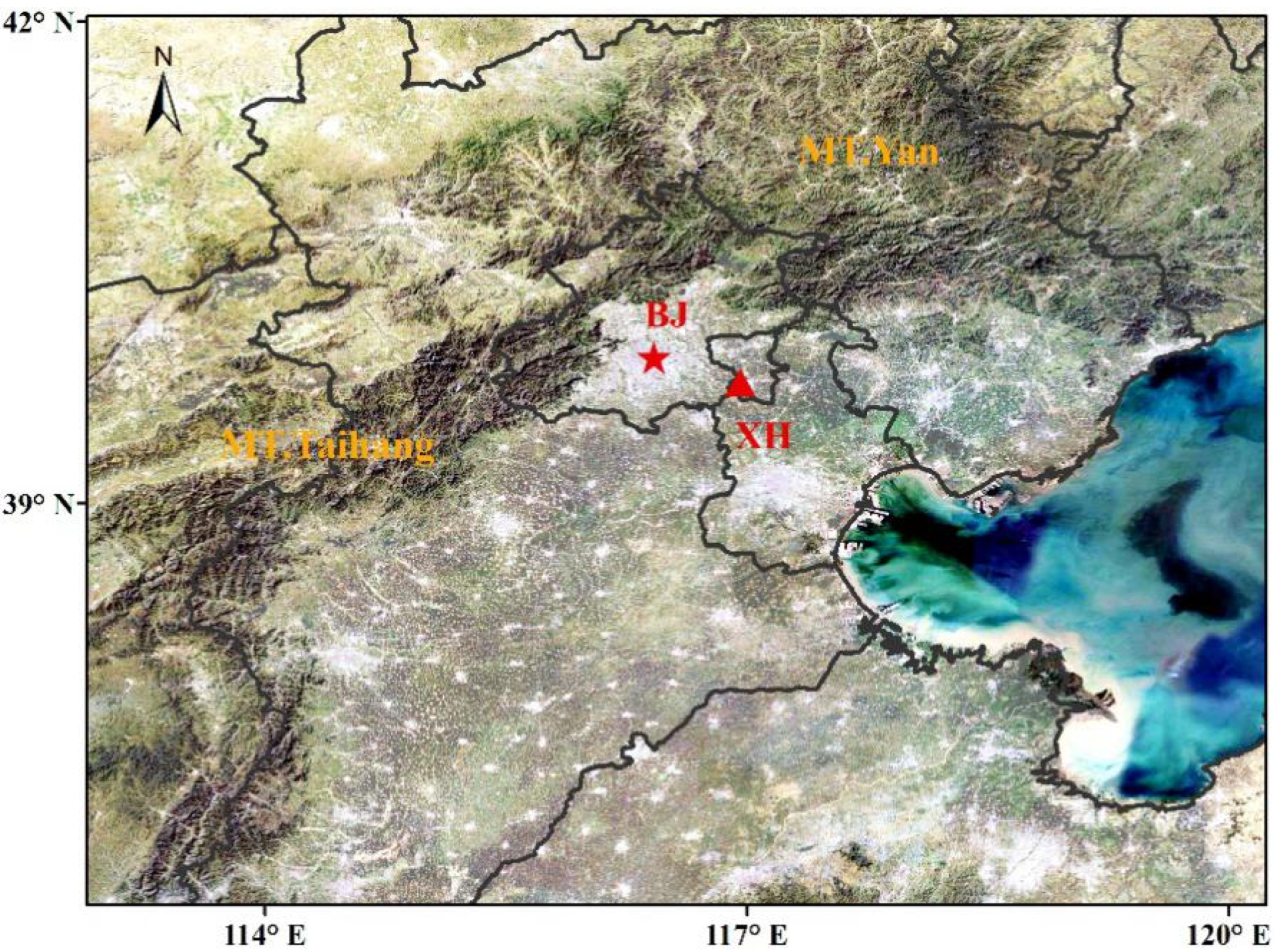
2.3. MAX-DOAS Measurements

Here, we present almost 2 years (from July 2019 to April 2021) of continuous MAX-DOAS NO₂ and SO₂ observations at the suburban station of Xianghe, China (39.8°N, 117.0°E), a representative site in a highly polluted area over North China Plain (NCP), about 50 km southeast of Beijing (see Figure 1). This MAX-DOAS instrument is designed by BIRA-IASB and operated by the Institute of Atmospheric Physics (IAP), Chinese Academy of Sciences. The MAX-DOAS focused on the zenith-sky DOAS technique and includes three main components: an optical head installed on a sun tracker, a thermo-regulated box consisting of two spectrometers, and two computers for equipment control and data storage [42]. This setup can measure both scattered and direct sunlight. One of the spectrometers works in UV band (300–390 nm) and another operates in VIS wavelength (400–720 nm). During the observation, the azimuth direction of the telescope is kept to the north. A complete measurement sequence contains 9 elevation viewing angles (2, 4, 6, 8, 10, 12, 15, 30 and 90°) and takes approximately 15 min.

In this study, the QDOAS, a spectral fitting software developed at BIRA-IASB, has been used to analyse the spectra observed from MAX-DOAS. The detailed configuration of retrieval is mentioned in

Table 1. Settings for NO₂ and SO₂ spectral fitting.

Parameter	Data Source	Trace Gas
		NO2	SO2
Fitting interval		425–490 nm	305–317.5 nm
Polynomial degree		5	5
NO2	[43], 220 K, 294 K	✓	✓ (only 294 K)
SO2	[44], 294 K	×	✓
O3	[45], 223 K, 243 K	✓ (only 243 K)	✓
O4	[46], 296 K	✓	×
H2O	[47], 298 K	✓	×
Ring	Calculated using QDOAS	✓	✓

. The fitting spectral ranges of NO₂ and SO₂ are 425–490 nm and 305–317.5 nm, respectively.

3. Methodology

3.1. Oversampling Method for OMI and TROPOMI L2 Data

To facilitate the comparison of different spaceborne data sources, various data need to be resampled to an equal spatial resolution. We use the inverse distance weighted interpolation (IDW) to resample the L2 satellite records into L3 grid data. Details could be seen in Wang et al. [30]. The distance ($D_i$) from the discrete point ($x_i$, $y_i$) to the established grid center point ($x_0$, $y_0$) can be defined as:

$$D_i=\sqrt{{\left(x_0-x_i\right)}^2+{\left(y_0-y_i\right)}^2}$$

(1)

and the estimation on grid point $Z_{\left(x_0, y_0\right)}$ can be calculated by:

$$Z_{\left(x_0, y_0\right)}={\displaystyle \sum }_{i=1}^n\frac{1}{{\left(D_i\right)}^P}{Z}_i/{\displaystyle \sum }_{i=1}^n\frac{1}{{\left(D_i\right)}^P}$$

(2)

where $Z_i$ is observed value on each pixel $i$, $N$ is the total counts of pixels involved in this calculation and $P$ represents the weight coefficient of distance.

Thus, the daily TROPOMI and OMI L2 observations were binned to 0.25° × 0.25° grids as the L3 datasets which are used in the subsequent verification, correction and related analysis.

3.2. Corrections Applied to TROPOMI L3 Data

It is assumed that the OMI and TROPOMI have similar observed results on tropospheric NO₂ and SO₂ columns, since these two instruments have analogous overpass times (13:45 LST for OMI and 13:30 LST for TROPOMI). Thus, to ensure reliable analysis in NCP area, we improve a mathematical correction method proposed by Huang and Sun [15] and revise the TROPOMI L3 data to reconcile the discrepancies with OMI.

For NO₂ correction, we obtained the 2-year average difference between OMI and TROPOMI L3 data in 2019 and 2020 as:

$$c_{\mathrm{n}}\left(i,j\right)={\mathrm{OMI}}_{2\mathrm{year}}\left(i,j\right)-{\mathrm{TROPOMI}}_{2\mathrm{year}}\left(i,j\right)$$

(3)

where $c_{\mathrm{n}}\left(i,j\right)$ is the mean difference of OMI minus TROPOMI in a grid. ${\mathrm{OMI}}_{2\mathrm{year}}$ and ${\mathrm{TROPOMI}}_{2\mathrm{year}}$ represent 2-year averages of L3 tropospheric NO₂ VCDs observed by OMI and TROPOMI, respectively, in 2019 and 2020. The correction item $c_{\mathrm{n}}\left(i,j\right)$ represents the probable sampling and algorithm biases between the different NO₂ products. The discussion of the stability of correction term is detailed in Section 4.1.

On the basis of Huang’s [15] method, we add a deviation coefficient $a_{\mathrm{n}}$ based on MAX-DOAS NO₂ results observed in Xianghe, which is defined as:

$$a_{\mathrm{n}}=\frac{{\mathrm{TROPOMI}}_{2\mathrm{year}}-{\mathrm{MAXDOAS}}_{2\mathrm{year}}}{\left[\left({\mathrm{TROPOMI}}_{2\mathrm{year}}-{\mathrm{MAXDOAS}}_{2\mathrm{year}}\right)+\left({\mathrm{OMI}}_{2\mathrm{year}}-{\mathrm{MAXDOAS}}_{2\mathrm{year}}\right)\right]}$$

(4)

Therefore, the corrected TROPOMI NO₂ in month (or year) $\mathrm{mi}$ could be expressed as:

$$\mathrm{TROPOMI}\_{\mathrm{corr}}_{\mathrm{mi}}\left(i,j\right)={\mathrm{TROPOMI}}_{\mathrm{mi}}\left(i,j\right)+a_{\mathrm{n}}\times c_{\mathrm{n}}\left(i,j\right)$$

(5)

The correction for TROPOMI SO₂ is the same as NO₂ correction. Thus, the correction factor $c_{\mathrm{s}}\left(i,j\right)$ for SO₂ is similar to $c_{\mathrm{n}}\left(i,j\right)$ which is mentioned in Equation (3), and the deviation coefficient $a_{\mathrm{s}}$ is also identical to $a_{\mathrm{n}}$ expressed in Equation (4). The correction method has been applied to correct the TROPOMI L3 dataset over the NCP region and relevant applications have been exhibited in Section 4.

4. Results

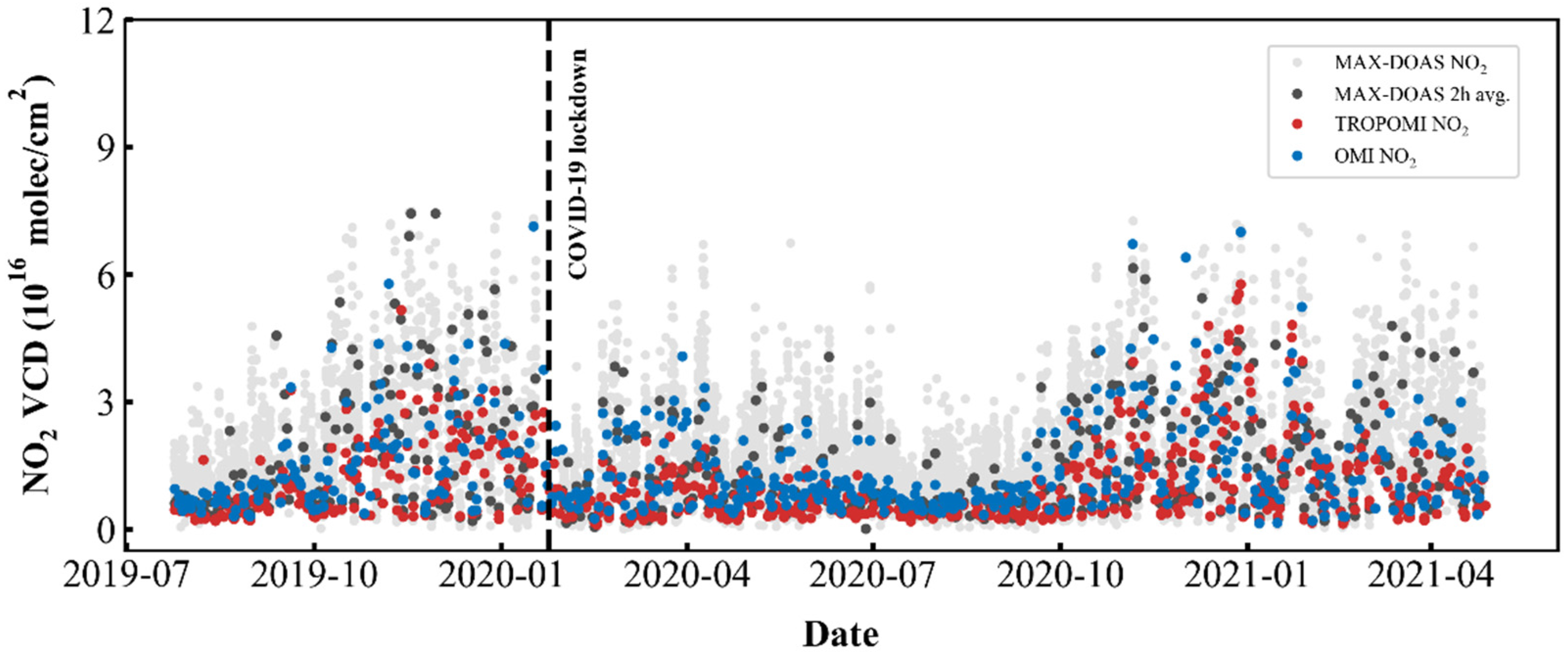
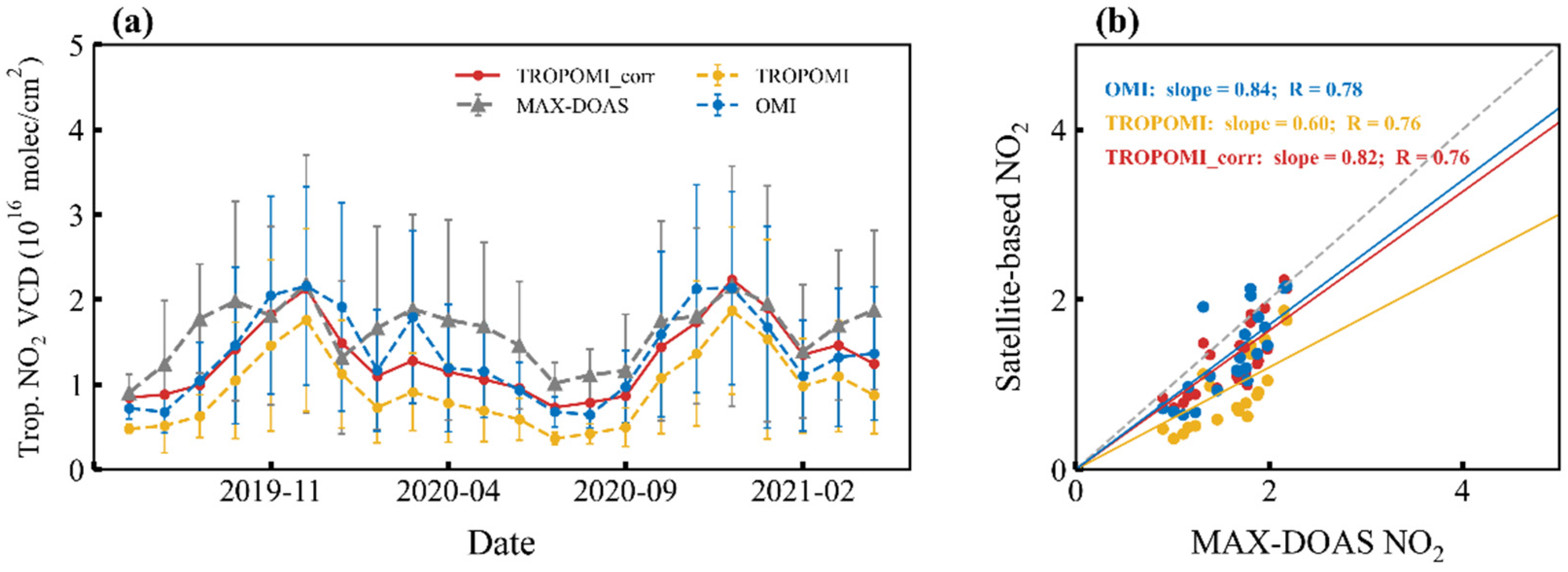
4.1. Evaluation and Correction for TROPOMI Tropospheric NO₂ Data

4.1.1. The Quality of TROPOMI NO₂ Data

The time series of TROPOMI (red dots), OMI (blue dots) tropospheric NO₂ data within a radius of 50 km around Xianghe observatory and the collocated MAX-DOAS measurements are indicated in Figure 2, covering the period July 2019 to April 2021. For MAX-DOAS NO₂ retrievals, we used full-day observed series (light grey dots) as well as the averaged values spanning 12:30 to 14:30 LST based on satellites’ overpass time (dark grey dots). The latter is used for quantitative comparison with satellite NO₂ columns. These three observations present the same peaks and mostly abide by the similar day-to-day variability, with maximum values during cold months.

Figure 3 employs the comparison of monthly mean NO₂ values between satellite and GB measurements as well as the corrected TROPOMI L3 datasets. Notably, the monthly mean data only comprised the coincident observation number of correlative days of three datasets. In general, both satellite and GB data show a similar tendency and a strong seasonality, with lowest NO₂ loadings in summer and highest in winter. The seasonality of NO₂ fluctuation is mainly related to the removal mechanisms of the OH radical, which has a similar seasonal cycle [26]. Moreover, satellited-based NO₂ unfolds negative biases relative to MAX-DOAS, and the OMI deviation is smaller and closer to the ground observation, ranging from 20% to 40%. TROPOMI tropospheric NO₂ VCDs are commonly lower than collocated MAX-DOAS by about 30–60%. This finding is consistent with the recent studies of Dimitropoulou et al. [48] and Wang et al. [30]. It is mainly because the representative scales are different between satellite and GB technique [32]. Correlation plots of all related measurements have been shown in Figure 3b. Despite showing negative drifts, the temporal patterns observed from OMI and TROPOMI closely match the GB measurements, since the correlation coefficient (R) values are 0.78 and 0.76 for monthly scales, respectively. The MAX-DOAS and OMI tropospheric NO₂ VCDs are highly correlated with the slope of 0.84, while the slope value (0.60) between MAX-DOAS and TROPOMI indicates that TROPOMI tends to be apparently underestimated.

Regarding the issue that TROPOMI NO₂ data are underestimated, previous works have investigated the origin of systematic uncertainties in TROPOMI NO₂ retrievals. Boersma et al. [49] presented that primary error sources are mainly attributed to the spectral fitting, the estimation of the stratospheric NO₂ content and uncertainties of ancillary parameters used in AMF calculation (i.e., cloud information, aerosols, surface albedo, and a priori NO₂ profile). For instance, Dimitropoulou et al. [48] discussed the effects of cloud, aerosol, surface albedo and a priori NO₂ profile on inversion results. Specifically, the cloud parameters are used as inputs in a cloud correction scheme applied to NO₂ retrieval that may lead to biases in the tropospheric NO₂ column. Furthermore, TROPOMI NO₂ inversion is prone to be affected by stricter cloud mask (named FRESCO-S) compared with OMI, which presumably removes some heavy pollution cases in the retrievals and induces an underestimation [30]. In addition, aerosols are considered indirectly in the TROPOMI NO₂ algorithm, which means aerosols are processed through the cloud correction scheme. Moreover, they changed the priori vertical profiles measured from MAX-DOAS to recalculate the satellite NO₂ VCDs, leading to a better correlation between the satellite and GB data. Overall, these factors all exert significant impacts on TROPOMI NO₂ inversion.

As a result, to reconcile the discrepancies, the approach shown in Section 3.2 are used to correct TROPOMI NO₂ L3 data. Compared to original results, the corrected TROPOMI results (TROPOMI_corr for short in Figure 3) are more consistent with MAX-DOS NO₂ column concentrations, with the slope being 0.82 (0.62 in original comparison).

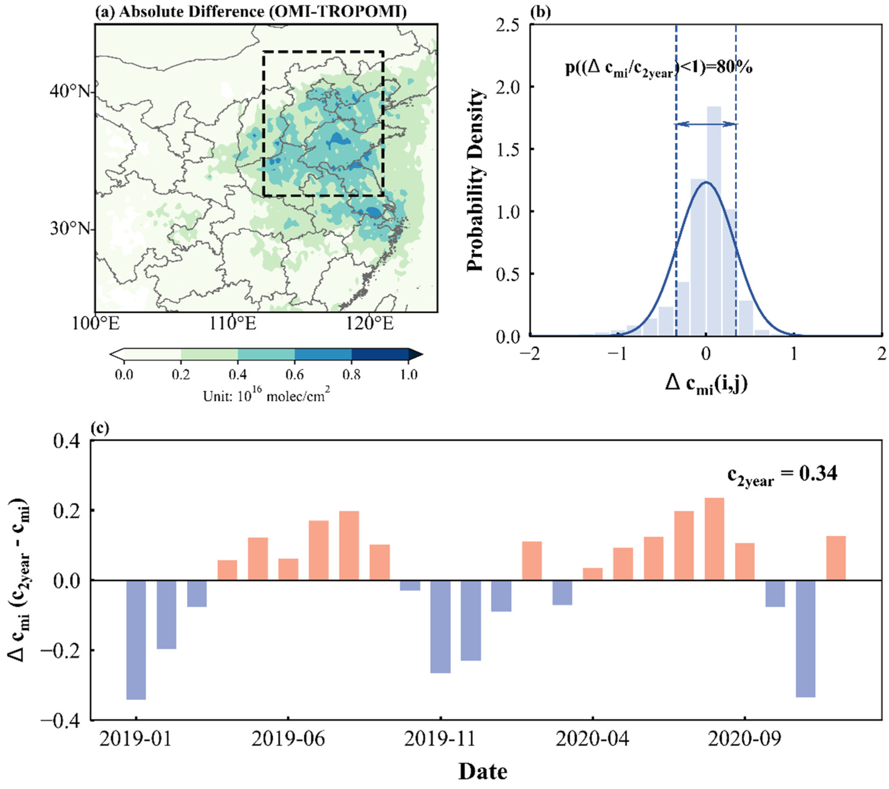
4.1.2. Feasibility Analysis of TROPOMI NO₂ Correction

In order to prove that the correction coefficient $c_{\mathrm{n}}\left(i,j\right)$ is stable within every month and could be used to correct TROPOMI L3 data over the NCP high polluted region, we define the deviation $\Delta c_{\mathrm{mi}}\left(i,j\right)$ as:

$$\Delta c_{\mathrm{mi}}\left(i,j\right)=c_{\mathrm{n}}\left(i,j\right)-c_{\mathrm{mi}}\left(i,j\right)$$

(6)

where $c_{\mathrm{mi}}\left(i,j\right)$ means the monthly average difference between OMI and TROPOMI of month $\mathrm{mi}$, and $\Delta c_{\mathrm{mi}}\left(i,j\right)$ denotes the deviation value in $c_{\mathrm{n}}$ and $c_{\mathrm{mi}}$ on each pixel $\left(i,j\right)$.

Throughout the two years combined, obvious differences prevail in Eastern China between TROPOMI and OMI as shown in panel (a) of Figure 4. Notably, tropospheric NO₂ values derived from the TROPOMI are lower than those from OMI at a nation-wide scale, especially in the NCP (black box highlighted in Figure 4a), where the discrepancies exceed 0.4 (×10¹⁶ molec cm⁻²). It means that the higher the NO₂ loadings the greater the underestimation. Considering the regionality of MAX-DOAS observations, we produce a corrected TROPOMI L3 dataset over the NCP region. The probability density distribution plot of $\Delta c_{\mathrm{mi}}\left(i,j\right)$ is reflected in Figure 4b. The $\Delta c_{\mathrm{mi}}\left(i,j\right)$ values denote the deviations derived from the 2-year average difference minus each monthly average difference (OMI-TROPOMI) over the NCP region during the study period, collected with all pixels. Evidently, approximately 80% of $\Delta c_{\mathrm{mi}}\left(i,j\right)$ values are lower than regional mean of $c_{\mathrm{n}}\left(i,j\right)$ values (denoted as $c_{2\mathrm{year}}$, about 0.34 × 10¹⁶ molec cm⁻²), indicating the feasibility of the correction term to some extent. Furthermore, the monthly change of regional mean of $\Delta c_{\mathrm{mi}}\left(i,j\right)$ is displayed in Figure 4c. The monthly deviation ranges from −0.3 to 0.2 (×10¹⁶ molec cm⁻²), with absolute values less than $c_{2\mathrm{year}}$. In addition, the positive difference mainly occurs in summer and spring, while the opposite often appears in winter and autumn. These results confirm that the $c_{\mathrm{n}}\left(i,j\right)$ could be used for TROPOMI NO₂ monthly mean data correction most of the time.

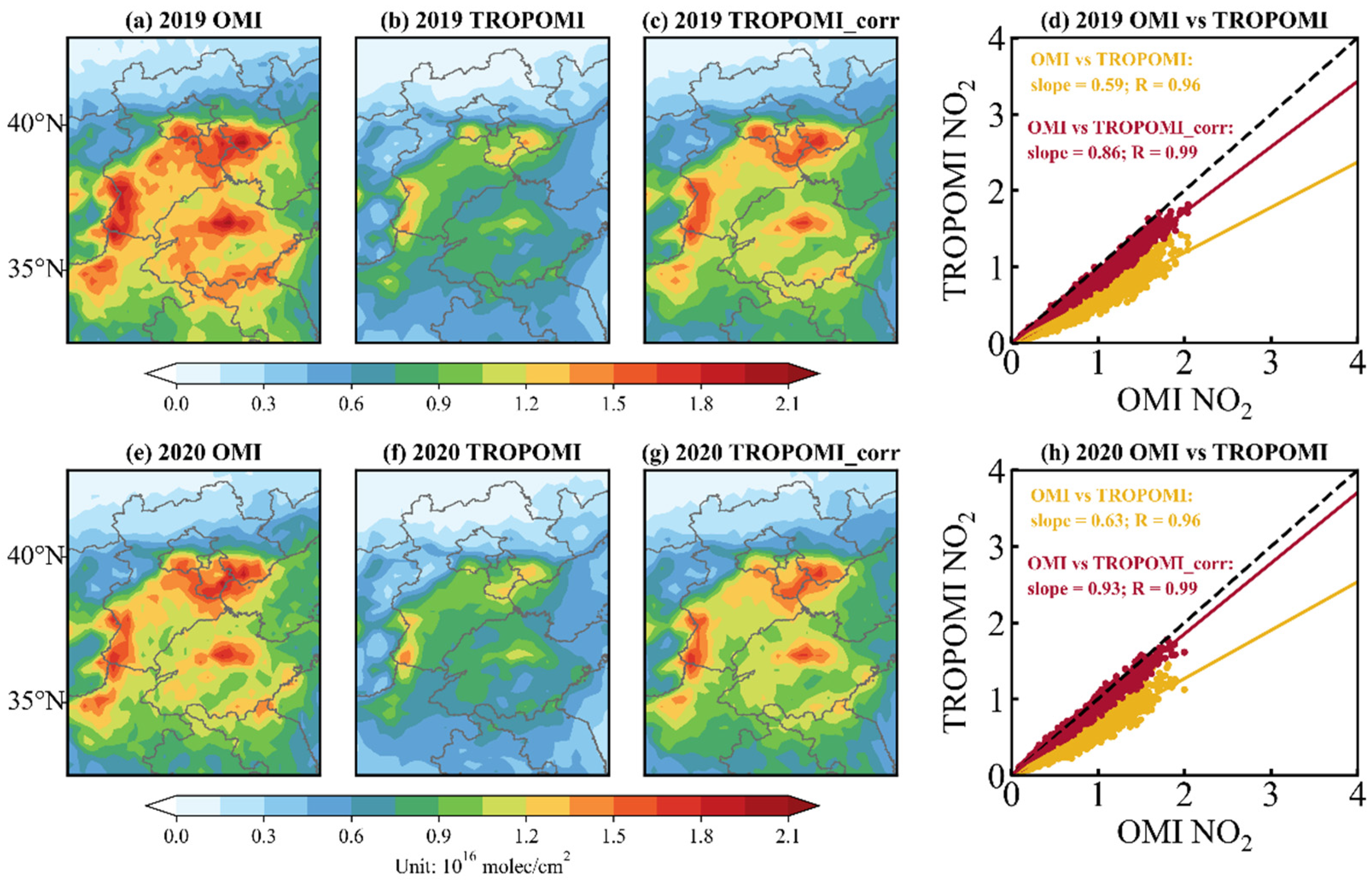
4.1.3. Correction for TROPOMI NO₂ over the NCP Region

Annual mean geographic distribution of tropospheric NO₂ VCDs over the NCP region observed from OMI, TROPOMI as well as the TROPOMI_corr are indicated in Figure 5a–c,e–g. The spatial structure from TROPOMI possesses a great resemblance to that from OMI, while the magnitudes in TROPOMI are lower than in OMI. High NO₂ loadings are mainly concentrated around provincial capitals with high emissions. Meanwhile, NO₂ declined significantly in most regions in 2020 compared with 2019, from both OMI and TROPOMI. Application of corrected TROPOMI NO₂ has improved significantly in magnitudes and shows better agreement with OMI observations. The linear regression (Figure 5d,h) yields that the slope of TROPOMI versus OMI increased from 0.59 to 0.86 in 2019 and from 0.63 to 0.93 in 2020. Furthermore, the correlation is much strengthened with the R values raised to 0.99 in these two years.

In brief summary, the TROPOMI, OMI and MAX-DOAS NO₂ VCDs exhibited similar temporal features during the study period at Xianghe site. Compared with GB measurements, the NO₂ VCDs derived from OMI had a regression slope (slope = 0.84) greater than that from TROPOMI (slope = 0.60). Moreover, focusing on the NCP region, the TROPOMI and OMI NO₂ VCDs were strongly correlated (R > 0.95) in terms of spatial pattern. However, the magnitudes in the TROPOMI are generally lower than in the OMI by 25% to 35%, particularly over highly contaminated areas in wintertime. Further, the corrected TROPOMI L3 NO₂ datasets have been greatly improved in magnitudes compared with MAX-DOAS and OMI considering either in a single point or over the entire region.

4.2. Evaluation and Correction for TROPOMI Total SO₂ Data

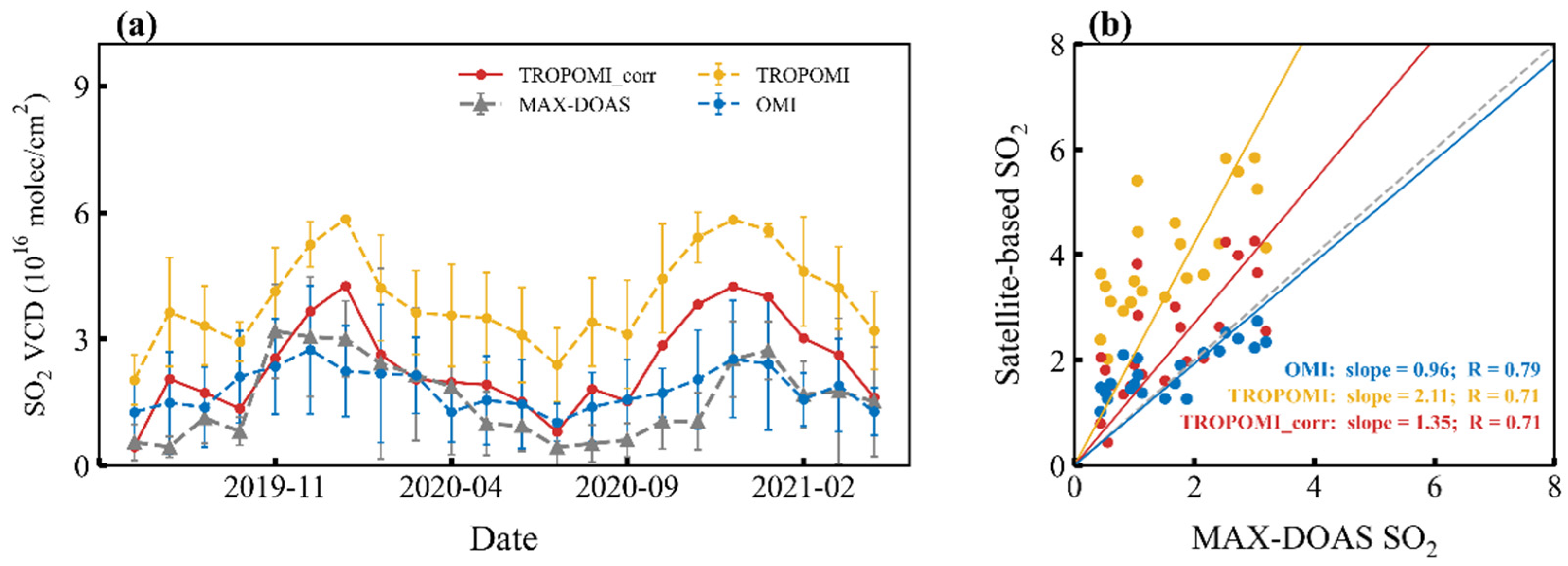
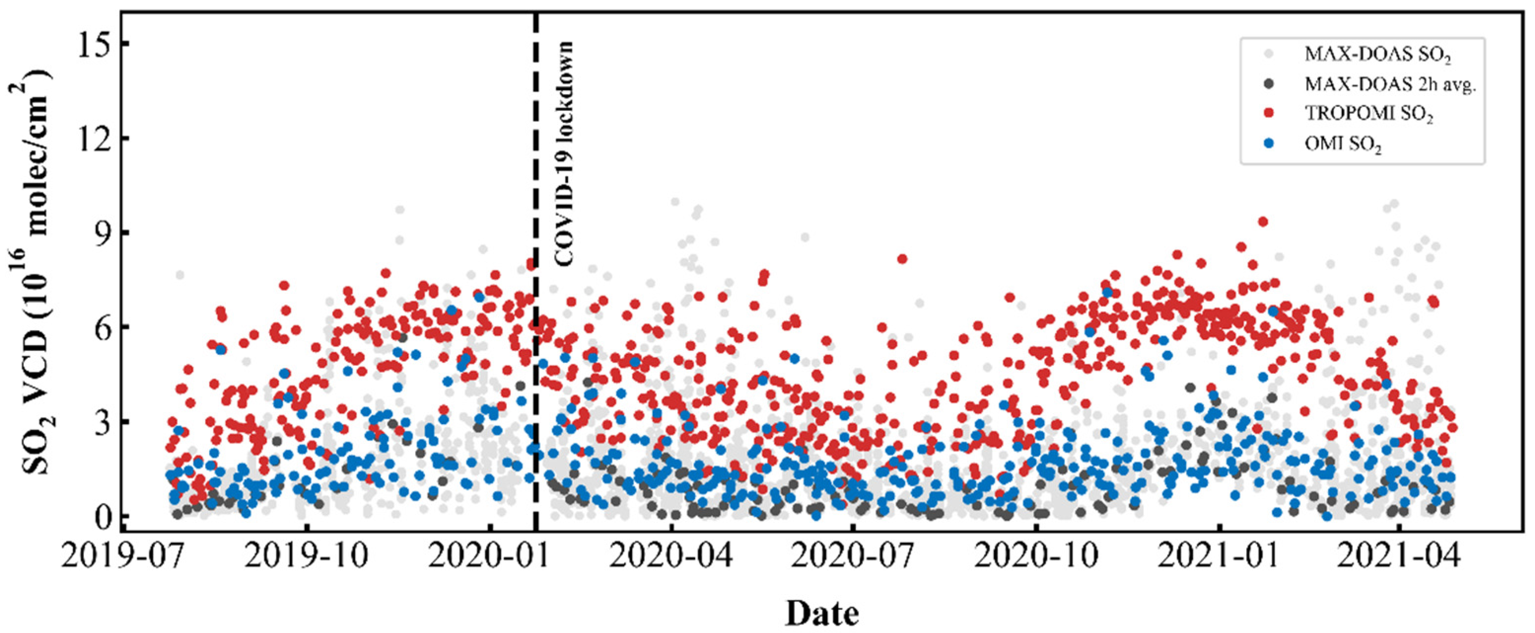
4.2.1. The Quality of TROPOMI SO₂ Data

Figure 6 shows the time series of SO₂ observations at the Xianghe site from July 2019 to April 2021. MAX-DOAS retrieved data are coincidentally averaged in approximately ±2 h (12:30 to 14:30 LST) overpass time of TROPOMI and OMI over the target region. The SO₂ VCDs show pronounced seasonal cycle, as evidenced by both remote sensing technique and GB measurement, with a maximum occurring in winter and autumn and a minimum in summer. This marked seasonal fluctuation can be explained by the seasonal feature of emission strengths and lifetimes of the SO₂ as well as the atmospheric transport [23,42]. Moreover, it is obvious that SO₂ VCDs derived from TROPOMI are apparently higher than that from OMI and MAX-DOAS.

To better explore SO₂ monthly variation and satellite product quality, the monthly SO₂ VCDs from space-based and GB measurements are performed. As shown in Figure 7, the monthly mean SO₂ columns from MAX-DOAS are well covariates with the OMI data (R = 0.79), and their magnitudes are in great agreement (slope = 0.96), implying well-captured monthly variations. In contrast, differences among TROPOMI-inferred SO₂ (marked in yellow line) and those of OMI and MAX-DOAS observations feature a slightly lower agreement (R = 0.71 with MAX-DOAS) and an order of magnitude difference (slope = 2.11 with MAX-DOAS) with TROPOMI typically overvalued. Based on the better consistency between the OMI and MAX-DOAS SO₂ VCDs, a method for TROPOMI SO₂ correction is developed.

In the following, we present the corrected SO₂ results derived from the correction technique introduced above (detailed in Section 3.2). The corresponding plot is also presented in Figure 7. For comparison of corrected TROPOMI and MAX-DOAS, slope is higher than 1 (slope = 1.35), suggesting that corrected TROPOMI observations still provide higher values than MAX-DOAS in several months, especially in wintertime. However, slope values of corrected SO₂ VCDs are close to 1 than that of original results (slope = 2.11), also indicating better agreement of corrected TROPOMI SO₂ in terms of monthly mean values.

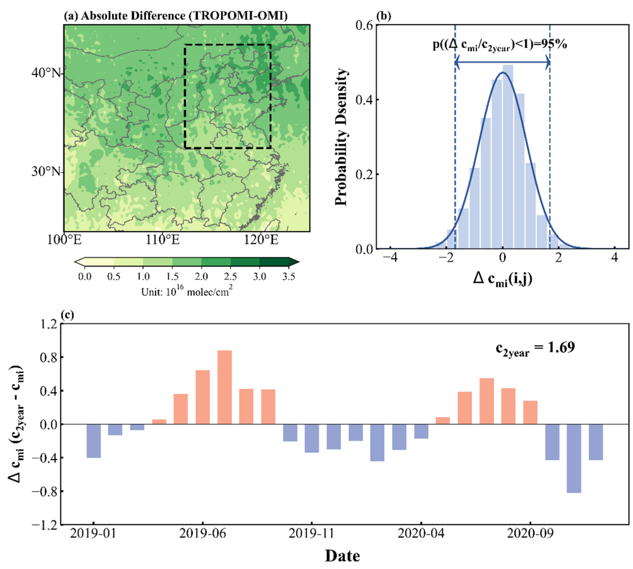
4.2.2. Feasibility Analysis of TROPOMI SO₂ Correction

Referring to the previous analysis, a verification for stability of correction coefficient $c_{\mathrm{s}}\left(i,j\right)$ was performed. As shown in Figure 8a, the absolute difference in SO₂ analysis is defined as TROPOMI minus OMI, which is different with in NO₂. The discrepancy is about 1.5 to 3.0 × 10¹⁶ molec cm⁻² over NCP area, indicating overestimated SO₂ values that are apparent in the TROPOMI measurements throughout the entire research area. Moreover, the TROPOMI SO₂ product exhibits severe SO₂ pollution in most areas of China, which is inconsistent with the fact that SO₂ emissions have been reduced significantly in China [50].

The probability density distribution plot of $\Delta c_{\mathrm{mi}}\left(i,j\right)$ is also shown in panel (b) of Figure 8. The definition of $\Delta c_{\mathrm{mi}}\left(i,j\right)$ for SO₂ is analogous to that of NO₂. As we can see, approximately 95% of $\Delta c_{\mathrm{mi}}\left(i,j\right)$ values are lower than regional mean of $c_{\mathrm{s}}\left(i,j\right)$ value (denoted as $c_{2\mathrm{year}}$, about 1.69 × 10¹⁶ molec cm⁻²), which means that the $c_{\mathrm{s}}\left(i,j\right)$ is reasonable to be used in each month correction. Considering the monthly change of regional mean of $\Delta c_{\mathrm{mi}}\left(i,j\right)$ in Figure 8c, the monthly deviation values are within ±0.8 (×10¹⁶ molec cm⁻²), larger than that of NO₂ (within ±0.3 × 10¹⁶ molec cm⁻²). Therefore, the magnitudes of the TROPOMI SO₂ retrievals need further correction and validation.

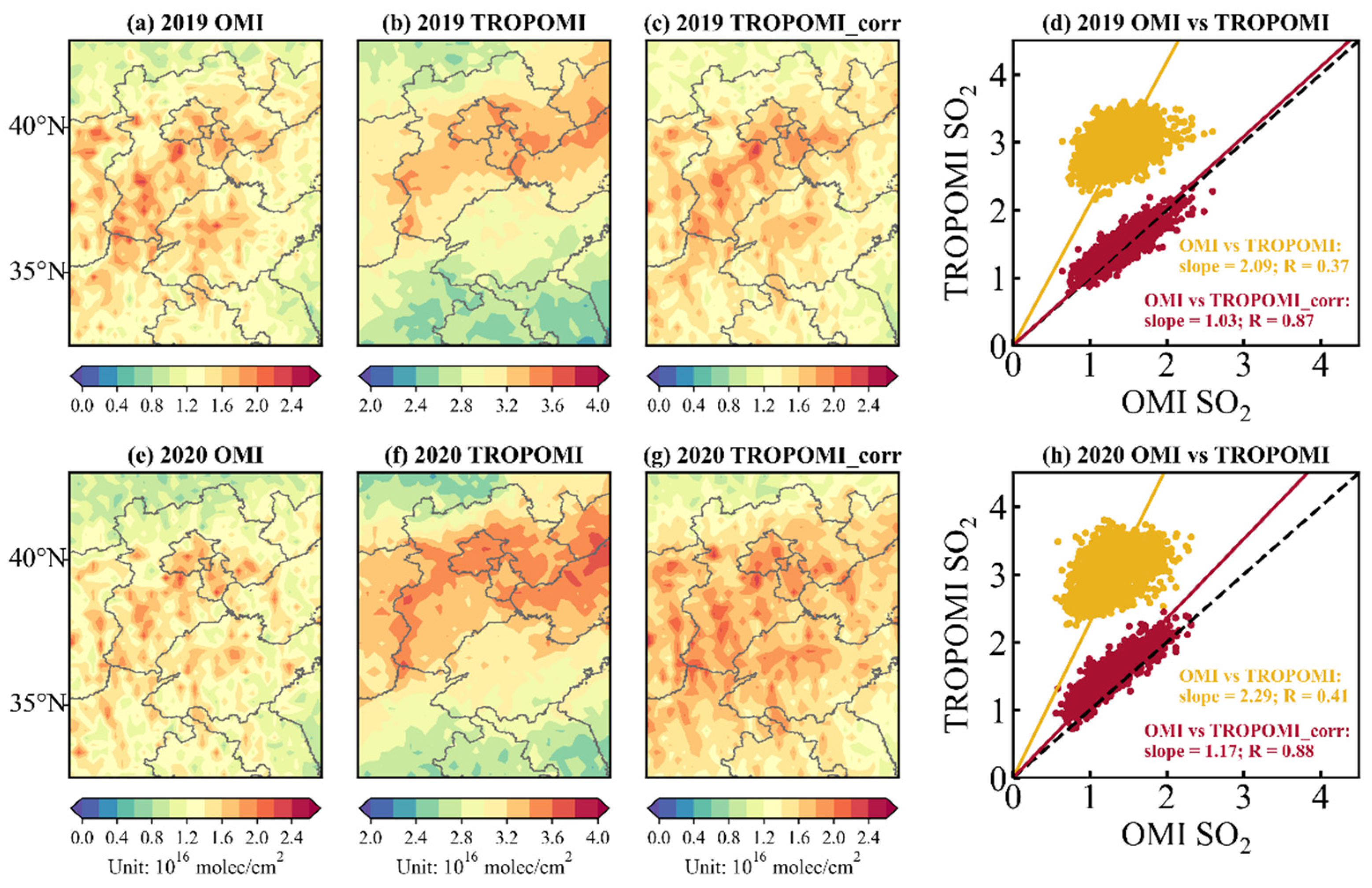
4.2.3. Correction for TROPOMI SO₂ over the NCP Region

Comparison results of TROPOMI, OMI and TROPOMI_corr SO₂ results in 2019 and 2020 are plotted in Figure 9. Large SO₂ columns are standing out over the NCP region. The retrievals by TROPOMI and OMI both reveal similar spatial distribution of the SO₂ loadings, while the magnitudes in TROPOMI are much higher than in OMI. In terms of the whole NCP area, the spatial correlations in annual mean SO₂ VCDs between the TROPOMI and OMI remained poor in some regions and the R values in 2019 and 2020 are 0.37 and 0.41, respectively. When the correction method is applied, TROPOMI SO₂ datasets are greatly improved, not only in regional distribution but also in magnitudes, with R values increased to above 0.85. As we know, the retrieval accuracy of SO₂ columns from TROPOMI is also limited by several factors, such as uncertainties of SCDs inversion and the AMF calculations. For instance, the SO₂ is not easy to be extracted as its low content in the atmosphere; and the absorption of SO₂ is weaker than that of O₃ in the equal wavelengths, which could be disturbed in the process of spectral fitting [50]. For another example, according to the research of Theys et al. [24], they considered potential factors causing errors in SO₂ retrievals, including the priori profile. They found that the OMI columns, which are corrected by the MAX-DOAS profile shape, agree very well with GB records. Moreover, Xia et al. [50] used a priori profile from GEOS-Chem schema instead of from TM5 simulations in TROPOMI SO₂ inversion, the relative bias between TROPOMI SO₂ results and MAX-DOAS observations descended from 17.9–28.4% to 11.2–12.4%. This illustrates the importance of a priori profiles on the SO₂ inversion.

In short, the TROPOMI inversions could capture the SO₂ temporal manners in general but tended to overstate the magnitudes over Xianghe observatory. For comparison of TROPOMI and OMI SO₂ over the NCP region, the apparent overestimation could also be found in TROPOMI, and weak spatial correlations (R < 0.45) were demonstrated. The corrected TROPOMI SO₂ L3 data are closer to OMI in magnitude and the correlation over the entire region has also increased. Inter-comparisons of the TROPOMI and MAX-DOAS SO₂ columns indicate that the inversion algorithm of TROPOMI SO₂ needs further improvement, especially in the heavily polluted areas over China.

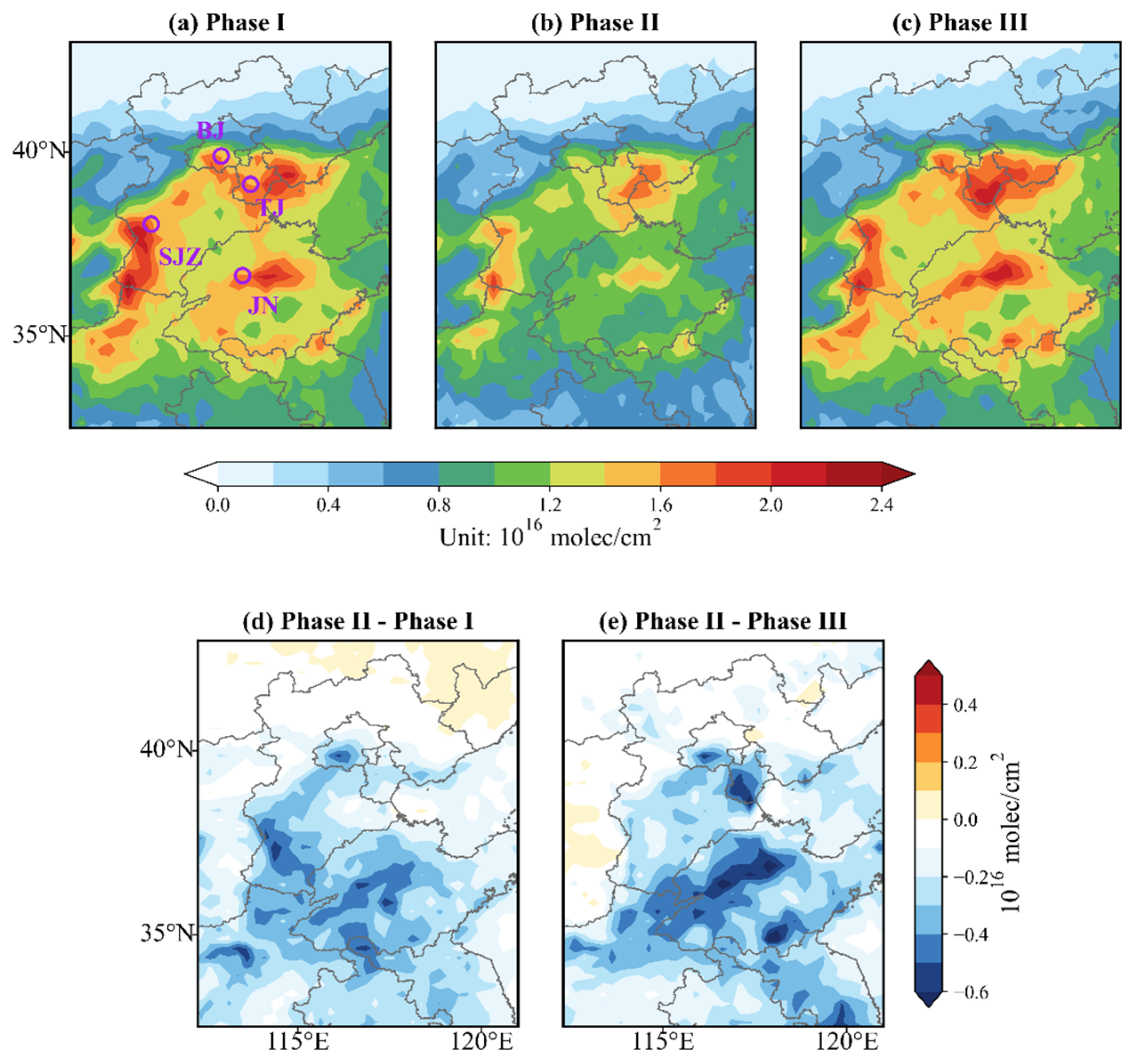
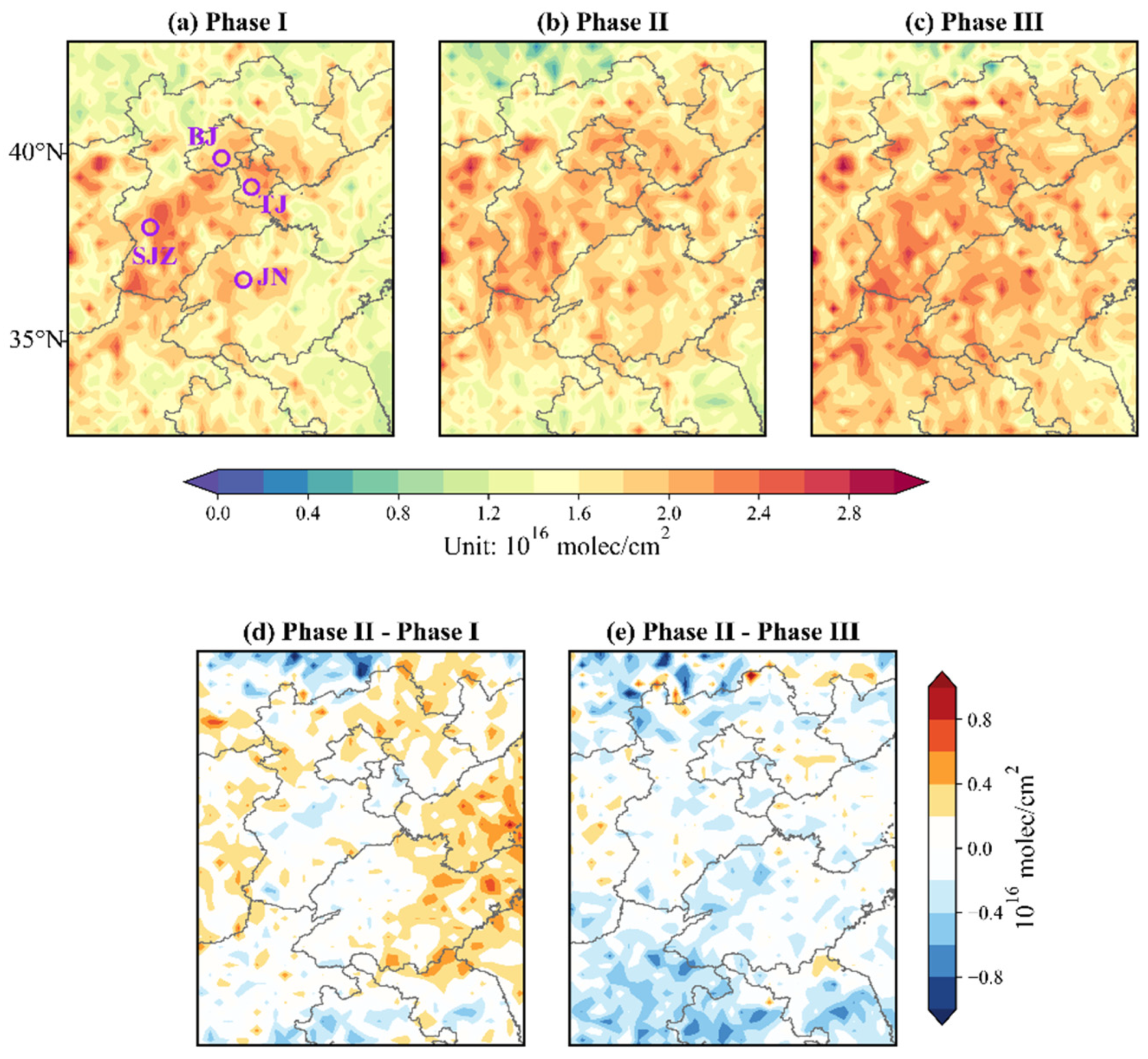
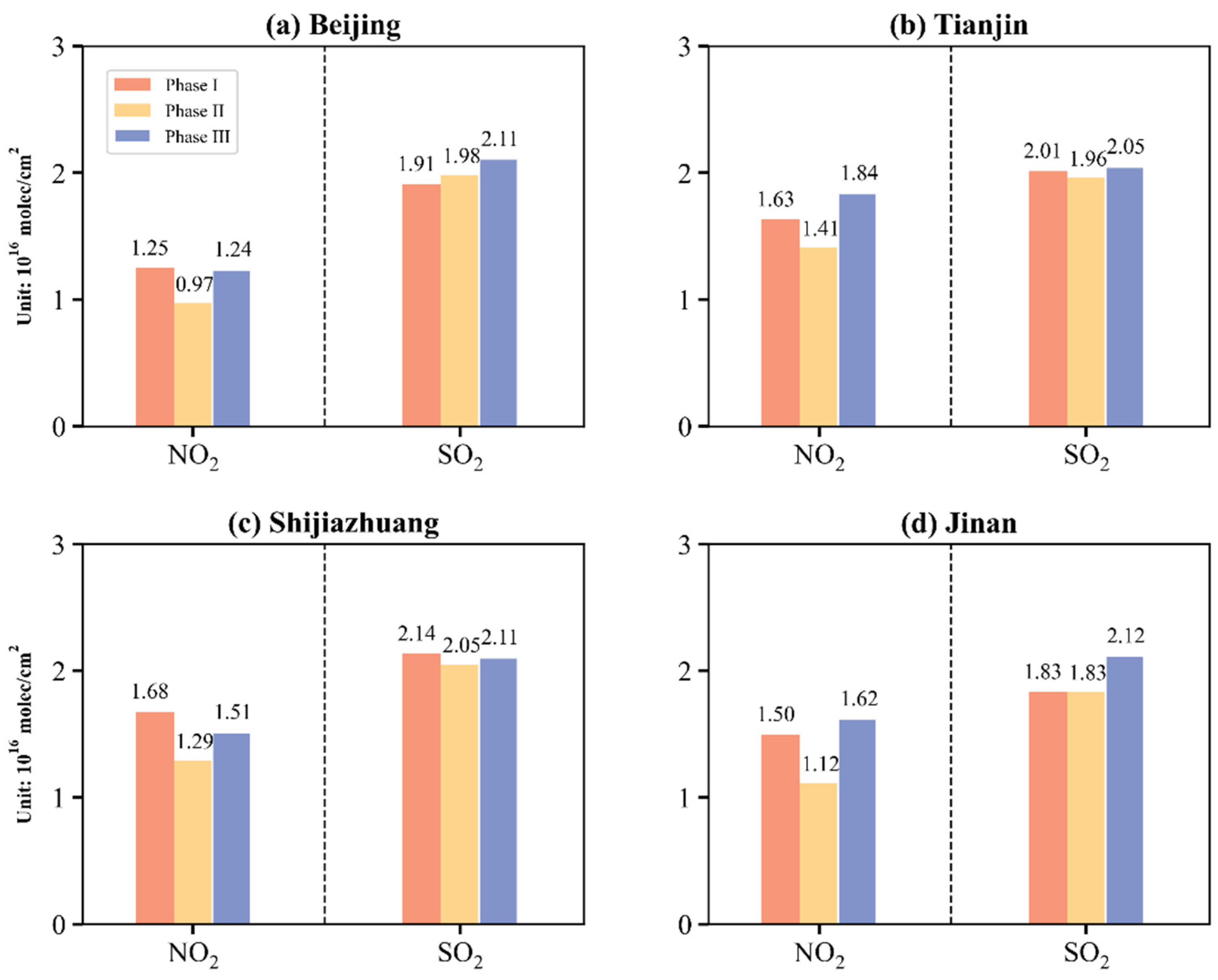
4.3. Analysis of NO₂ and SO₂ over NCP during COVID-19 Period

The global lockdown caused by the coronavirus disease (COVID-19) pandemic in 2020 reduced social and economic activities in China. The Chinese government implemented a strict lockdown measure in Wuhan on January 23. By then, a lockdown was enforced in Wuhan and extended to nationwide until 8 April 2020. Based on the corrected NO₂ and SO₂ TROPOMI L3 datasets, we investigated the responses of the NO₂ and SO₂ levels resulting from the spread of COVID-19 over the NCP region. Average NO₂ columns during January to April in 2019, 2020 (lockdown period) and 2021 are referred to as Phase I, Phase II and Phase III, respectively. Note that the lunar new year holidays in 2019 range from 4 February to 10 February, in 2020 from 24 January to 31 January, and in 2021 from 11 February to 17 February, which are all included in our research period. Therefore, the impact of “holiday effect” is not considered separately.

Figure 10 presents the spatial pattern of time-averaged NO₂ columns over NCP into three phases. Regarding NO₂, high contents are shown in the provincial capitals and their surrounding areas, and broad-scale reductions by 25% to 45% are prevalent in NCP during Phase II. The reduction pattern shown in Figure 10d implies a substantial reduction in economic activities and human migration during this period. During Phase III, when the epidemic prevention and control gradually alleviated, the NO₂ concentrations exhibit a rapid and sharp increase, with highest amplification in the areas surrounding Tianjin (TJ) and Jinan (JN) by about up to 60%. Overall, the lockdown measure during COVID-19 had a significant effect on NO₂ reductions over the entire NCP area. After that, a prominent rebound trend was noted in the same period in 2021.

According to the NO₂ decrease, a SO₂ reduction is also be expected during COVID-19. However, unlike previous conclusions, SO₂ columns did not change obviously during the blockade period. As shown in Figure 11, compared to Phase I, the differences in most areas are about −0.4 to 0.4 × 10¹⁶ molec cm⁻² (approximately −0.15 to 0.15 DU, 1 DU = 2.687 × 10¹⁶ molec cm⁻²), suggesting that SO₂ concentration remains fairly stable throughout Phase I and Phase II. Taking into account Phase III, the SO₂ columns still keep stable compared with Phase II, with slightly increased only in some places about 10–20%. It manifests that control measures during COVID-19 have negligible impact on atmospheric SO₂.

In general, high NO₂ accumulation was similar to SO₂, which may appear over the similar hot spots in North China. For quantitative comparison, four major capital cities over this target region have been given and discussed in Figure 12. The tropospheric NO₂ columns in all spots experienced a dramatic drop during Phase II and then recovered progressively. Specifically, the NO₂ VCDs decreased by 0.28, 0.22, 0.39 and 0.38 × 10¹⁶ molec cm⁻² in Beijing (BJ), TJ, Shijiazhuang (SJZ) and JN areas, respectively, between Phase I and Phase II, reflecting overall lower emissions during this period. Then, significant growth appeared in phase III, indicating that a recovery to previous years after the epidemic remission is expected. As for SO₂, the columns in the lockdown period (Phase II) have changed little versus during the same period of Phase I. Subsequently, in Phase III, SO₂ levels in the four regions increased slightly, with the highest increase in JN by about 15.8%.

In sum, the NO₂ levels during Phase II were overall significantly lower than in Phase I, and the NO₂ levels may quickly rebound when public activities in China are resumed. However, SO₂ changes were less pronounced during COVID-19. Thus, the restrictive measures that China had implemented to respond to COVID-19 had a more obvious influence on NO₂. In addition, although the air quality has been improved in the short term due to the lockdown measures during COVID-19, the pollution status will rebound to its previous level at once the industrial and human activities return to normal levels.

5. Discussion

The results from the present comparison analysis could improve our understanding of the quality of TROPOMI products in China, especially the validation and investigation of SO₂, which is still scarce in current research.

Throughout the analysis above, we found that both the diurnal and monthly NO₂ and SO₂ variability are revealed well by the TROPOMI, in accordance with OMI and MAX-DOAS measurements in Xianghe site, displaying an evident seasonal characteristic with highest in winter and lowest in summer. However, some uncertainties also exist over highly polluted areas, especially for SO₂ data, which cannot well reflect the current pollution status in China. Therefore, combining with other satellite and ground-based dataset, we provided an attempt to correct TROPOMI dataset, hoping to improve its accuracy and make it more consistent with the real pollution situation in China. In other parts of China, this method could also be applied with reliable satellite and ground-based data. In addition, we need to realize that the error source analysis of TROPOMI data products and the improvement of algorithm process over China are still necessary.

When using the modified dataset to study the environmental pollution situation before and after COVID-19 over the NCP area, we found that NO₂ experienced a process of rising first and then reducing. In fact, several epidemic-related studies have confirmed the fact that NO₂ levels decreased significantly during COVID-19 in 2020, as shown in Bauwens et al. [13], Fan et al. [14], Huang and Sun [15] and Filonchyk et al. [51]. In this study, a comparison of the same period in 2021 also confirms that NO₂ has returned to pre-epidemic (in 2019) levels without the strict lockdown policy. In contrast, SO₂ concentrations did not fluctuate significantly before and after COVID-19. Although, in the study of Fan et al. [14] and Filonchyk et al. [51], slight declines in SO₂ concentrations also appeared in certain areas and cities during COVOD-19 (in 2020). However, compared with the sharp decline of NO₂, the change of SO₂ seems not obvious. Considering the reasons for this phenomenon, we also made some reasonable guesses. As mentioned in Filonchyk et al. [51], they showed that SO₂ levels decreased slightly in February 2020, compared with February 2019, and coal consumption in power plants and factories recovered to previous levels by the end of March, restoring SO₂ levels to normal. In addition, at the same stage in 2021, SO₂ still remains stable, and similar finding is also mentioned in the study of Wang et al. [52]. They found that SO₂ changes were not statistically significant over the NCP region during the Asian-Pacific Economic Cooperation (APEC) in 2014, showing that the SO₂ reduction was more related to natural or random variability rather than external forcing. Similarly, the specific factors causing such changes in NO₂ and SO₂ during COVID-19 still need further experiments and discussions.

6. Conclusions

In this study, column NO₂ and SO₂ data derived from TROPOMI/S5P were evaluated against ground-based MAX-DOAS at a single site (Xianghe) from 2019 to 2021. Comparison between TROPOMI retrievals and OMI products over a highly polluted region (NCP) are also conducted. It was found that satellited-based NO₂ data are both negatively biased relative to MAX-DOAS, and the OMI deviation is smaller and closer to the ground observation, ranging from 20% to 40%. Meanwhile, TROPOMI tropospheric NO₂ VCDs are slightly lower than collocated MAX-DOAS observations by about 30–60%. When it comes to SO₂, the monthly average SO₂ column retrieved from TROPOMI is larger than MAX-DOAS and OMI, with a mean bias of 2.41 (153.8%) and 2.17 × 10¹⁶ molec cm⁻² (120.7%) at Xianghe site, respectively. MAX-DOAS comparisons to OMI are more correlated than TROPOMI during the investigated time (R = 0.79 vs. 0.71). SO₂ VCDs derived from TROPOMI seem overestimated and the algorithm needs to be further improved in the future.

After the correction, TROPOMI NO₂ and SO₂ displayed markedly better consistencies with OMI in both magnitudes and distribution over the NCP area. The R values for regional mean concentrations increased greater than 0.95 and 0.85 for NO₂ and SO₂, respectively.

Finally, we used the corrected TROPOMI NO₂ and SO₂ dataset to investigate the environmental pollution status during COVID-19 period over the NCP region. Evident decreases in NO₂ columns were shown in the lockdown period (Phase II) compared to the same period in 2019 (Phase I), reduced by almost 25–45%, while SO₂ concentration remains fairly stable throughout Phase I and Phase II. Then, NO₂ and SO₂ levels observed from TROPOMI returned to normal in Phase III. This implies that the lockdown measure during COVID-19 had a certain inhibitory effect on environmental pollution and are expected to be more effective on NO₂ reduction than SO₂. Although the air quality was improved in the short term due to the lockdown measures during COVID-19, the pollution levels may rebound to their previous level once industrial and human activities return to original levels.

Overall, these works will help the assessment and algorithm improvement work for future TROPOMI NO₂ and SO₂ products, and further studies are also needed to investigate the causes of such errors of the NO₂ and SO₂ inversion over China.

References

1. Schneider, P.; Lahoz, W.A.; van der A, R. Recent satellite-based trends of tropospheric nitrogen dioxide over large urban agglomerations worldwide. Atmos. Chem. Phys. 2015, 15, 1205–1220. [Google Scholar] [CrossRef] [Green Version]
2. Krotkov, N.A.; Mclinden, C.A.; Li, C.; Lamsal, L.N.; Streets, D.G. Aura OMI observations of regional SO2 and NO2 pollution changes from 2005 to 2015. Atmos. Chem. Phys. 2016, 16, 4605–4629. [Google Scholar] [CrossRef] [Green Version]
3. Meng, K.; Xu, X.; Cheng, X.; Xu, X.; Qu, X.; Zhu, W.; Ma, C.; Yang, Y.; Zhao, Y. Spatio-temporal variations in SO2 and NO2 emissions caused by heating over the Beijing-Tianjin-Hebei Region constrained by an adaptive nudging method with OMI data. Sci. Total Environ. 2018, 642, 543–552. [Google Scholar] [CrossRef] [PubMed]
4. Zhang, X.; van Geffen, J.; Liao, H.; Zhang, P.; Lou, S. Spatiotemporal variations of tropospheric SO2 over China by SCIAMACHY observations during 2004–2009. Atmos. Environ. 2012, 60, 238–246. [Google Scholar] [CrossRef]
5. Zhao, P.; Tuygun, G.T.; Li, B.; Liu, J.; Yuan, L.; Luo, Y.; Xiao, H.; Zhou, Y. The effect of environmental regulations on air quality: A long-term trend analysis of SO2 and NO2 in the largest urban agglomeration in southwest China. Atmos. Pollut. Res. 2019, 10, 2030–2039. [Google Scholar] [CrossRef]
6. Wang, C.; Wang, T.; Wang, P. The Spatial–Temporal Variation of Tropospheric NO2 over China during 2005 to 2018. Atmosphere 2019, 10, 444. [Google Scholar] [CrossRef] [Green Version]
7. Lu, Z.; Streets, D.G.; Zhang, Q.; Wang, S.; Carmichael, G.R.; Cheng, Y.F.; Wei, C.; Chin, M.; Diehl, T.; Tan, Q. Sulfur dioxide emissions in China and sulfur trends in East Asia since 2000. Atmos. Chem. Phys. 2010, 10, 6311–6331. [Google Scholar] [CrossRef] [Green Version]
8. Li, C.; Zhang, Q.; Krotkov, N.A.; Streets, D.G.; He, K.; Tsay, S.-C.; Gleason, J.F. Recent large reduction in sulfur dioxide emissions from Chinese power plants observed by the Ozone Monitoring Instrument. Geophys. Res. Lett. 2010, 37. [Google Scholar] [CrossRef] [Green Version]
9. Zhang, Q.; Geng, G.; Wang, S.; Richter, A.; He, K. Satellite remote sensing of changes in NO x emissions over China during 1996–2010. Chin. Sci. Bull. 2012, 57, 2857–2864. [Google Scholar] [CrossRef] [Green Version]
10. Koukouli, M.E.; Balis, D.S.; van der A, R.J.; Theys, N.; Hedelt, P.; Richter, A.; Krotkov, N.; Li, C.; Taylor, M. Anthropogenic sulphur dioxide load over China as observed from different satellite sensors. Atmos. Environ. 2016, 145, 45–59. [Google Scholar] [CrossRef]
11. Wang, T.; Wang, P.; Theys, N.; Tong, D.; Hendrick, F.; Zhang, Q.; Van Roozendael, M. Spatial and temporal changes in SO2 regimes over China in the recent decade and the driving mechanism. Atmos. Chem. Phys. 2018, 18, 18063–18078. [Google Scholar] [CrossRef] [Green Version]
12. van der A, R.J.; Mijling, B.; Ding, J.; Koukouli, M.E.; Liu, F.; Li, Q.; Mao, H.; Theys, N. Cleaning up the air: Effectiveness of air quality policy for SO2 and NOx emissions in China. Atmos. Chem. Phys. 2017, 17, 1775–1789. [Google Scholar] [CrossRef] [Green Version]
13. Bauwens, M.; Compernolle, S.; Stavrakou, T.; Müller, J.F.; Van Gent, J.; Eskes, H.; Levelt, P.F.; van der A, R.; Veefkind, J.P.; Vlietinck, J.; et al. Impact of coronavirus outbreak on NO2 pollution assessed using TROPOMI and OMI observations. Geophys. Res. Lett. 2020, 47, e2020GL087978. [Google Scholar] [CrossRef]
14. Fan, C.; Li, Y.; Guang, J.; Li, Z.; Elnashar, A.; Allam, M.; de Leeuw, G. The Impact of the Control Measures during the COVID-19 Outbreak on Air Pollution in China. Remote Sens. 2020, 12, 1613. [Google Scholar] [CrossRef]
15. Huang, G.; Sun, K. Non-negligible impacts of clean air regulations on the reduction of tropospheric NO2 over East China during the COVID-19 pandemic observed by OMI and TROPOMI. Sci. Total Environ. 2020, 745, 141023. [Google Scholar] [CrossRef] [PubMed]
16. Sarfraz, M.; Mohsin, M.; Naseem, S.; Kumar, A. Modeling the relationship between carbon emissions and environmental sustainability during COVID-19: A new evidence from asymmetric ARDL cointegration approach. Environ. Dev. Sustain. 2021, 23, 16208–16226. [Google Scholar] [CrossRef]
17. Schneider, P.; van der A, R.J. A global single-sensor analysis of 2002-2011 tropospheric nitrogen dioxide trends observed from space. J. Geophys. Res. Atmos. 2012, 117, D16309. [Google Scholar] [CrossRef] [Green Version]
18. Geddes, J.A.; Martin, R.V. Global deposition of total reactive nitrogen oxides from 1996 to 2014 constrained with satellite observations of NO2; columns. Atmos. Chem. Phys. 2017, 17, 10071–10091. [Google Scholar] [CrossRef] [Green Version]
19. van der A, R.J.; Peters, D.H.M.U.; Eskes, H.; Boersma, K.F.; Van Roozendael, M.; De Smedt, I.; Kelder, H.M. Detection of the trend and seasonal variation in tropospheric NO2 over China. J. Geophys. Res. 2006, 111, D12317. [Google Scholar] [CrossRef] [Green Version]
20. Queisser, M.; Burton, M.; Theys, N.; Pardini, F.; Salerno, G.; Caltabiano, T.; Varnam, M.; Esse, B.; Kazahaya, R. TROPOMI enables high resolution SO2 flux observations from Mt. Etna, Italy, and beyond. Sci. Rep. 2019, 9, 957. [Google Scholar] [CrossRef]
21. Fioletov, V.E.; McLinden, C.A.; Krotkov, N.; Moran, M.D.; Yang, K. Estimation of SO2 emissions using OMI retrievals. Geophys. Res. Lett. 2011, 38, L21811. [Google Scholar] [CrossRef]
22. Wang, S.W.; Zhang, Q.; Streets, D.G.; He, K.B.; Martin, R.V.; Lamsal, L.N.; Chen, D.; Lei, Y.; Lu, Z. Growth in NOx emissions from power plants in China: Bottom-up estimates and satellite observations. Atmos. Chem. Phys. 2012, 12, 4429–4447. [Google Scholar] [CrossRef] [Green Version]
23. Jin, J.; Ma, J.; Lin, W.; Zhao, H.; Shaiganfar, R.; Beirle, S.; Wagner, T. MAX-DOAS measurements and satellite validation of tropospheric NO2 and SO2 vertical column densities at a rural site of North China. Atmos. Environ. 2016, 133, 12–25. [Google Scholar] [CrossRef]
24. Theys, N.; De Smedt, I.; Van Gent, J.; Danckaert, T.; Wang, T.; Hendrick, F.; Stavrakou, T.; Bauduin, S.; Clarisse, L.; Li, C.; et al. Sulfur dioxide vertical column DOAS retrievals from the Ozone Monitoring Instrument: Global observations and comparison to ground-based and satellite data. J. Geophys. Res. Atmos. 2015, 120, 2470–2491. [Google Scholar] [CrossRef]
25. Irie, H.; Takashima, H.; Kanaya, Y.; Boersma, K.F.; Gast, L.; Wittrock, F.; Brunner, D.; Zhou, Y.; Van Roozendael, M. Eight-component retrievals from ground-based MAX-DOAS observations. Atmos. Meas. Tech. 2011, 4, 1027–1044. [Google Scholar] [CrossRef] [Green Version]
26. Tian, X.; Xie, P.; Xu, J.; Li, A.; Wang, Y.; Qin, M.; Hu, Z. Long-term observations of tropospheric NO2, SO2 and HCHO by MAX-DOAS in Yangtze River Delta area, China. J. Environ. Sci. 2018, 71, 207–221. [Google Scholar] [CrossRef]
27. Chan, K.L.; Wang, Z.; Ding, A.; Heue, K.P.; Shen, Y.; Wang, J.; Zhang, F.; Shi, Y.; Hao, N.; Wenig, M. MAX-DOAS measurements of tropospheric NO2; and HCHO in Nanjing and a comparison to ozone monitoring instrument observations. Atmos. Chem. Phys. 2019, 19, 10051–10071. [Google Scholar] [CrossRef] [Green Version]
28. Griffin, D.; Zhao, X.; McLinden, C.A.; Boersma, F.; Bourassa, A.; Dammers, E.; Degenstein, D.; Eskes, H.; Fehr, L.; Fioletov, V.; et al. High-Resolution Mapping of Nitrogen Dioxide With TROPOMI: First Results and Validation Over the Canadian Oil Sands. Geophys. Res. Lett. 2019, 46, 1049–1060. [Google Scholar] [CrossRef] [Green Version]
29. Verhoelst, T.; Compernolle, S.; Pinardi, G.; Lambert, J.C.; Eskes, H.J.; Eichmann, K.U.; Fjæraa, A.M.; Granville, J.; Niemeijer, S.; Cede, A.; et al. Ground-based validation of the Copernicus Sentinel-5P TROPOMI NO2 measurements with the NDACC ZSL-DOAS, MAX-DOAS and Pandonia global networks. Atmos. Meas. Tech. 2021, 14, 481–510. [Google Scholar] [CrossRef]
30. Wang, C.; Wang, T.; Wang, P.; Rakitin, V. Comparison and Validation of TROPOMI and OMI NO2 Observations over China. Atmosphere 2020, 11, 636. [Google Scholar] [CrossRef]
31. Zhao, X.; Griffin, D.; Fioletov, V.; McLinden, C.; Cede, A.; Tiefengraber, M.; Müller, M.; Bognar, K.; Strong, K.; Boersma, F.; et al. Assessment of the quality of TROPOMI high-spatial-resolution NO2 data products in the Greater Toronto Area. Atmos. Meas. Tech. 2020, 13, 2131–2159. [Google Scholar] [CrossRef]
32. Ialongo, I.; Virta, H.; Eskes, H.; Hovila, J.; Douros, J. Comparison of TROPOMI/Sentinel-5 Precursor NO2 observations with ground-based measurements in Helsinki. Atmos. Meas. Tech. 2020, 13, 205–218. [Google Scholar] [CrossRef] [Green Version]
33. Judd, L.M.; Al-Saadi, J.A.; Szykman, J.J.; Valin, L.C.; Janz, S.J.; Kowalewski, M.G.; Eskes, H.J.; Veefkind, J.P.; Cede, A.; Mueller, M.; et al. Evaluating Sentinel-5P TROPOMI tropospheric NO2 column densities with airborne and Pandora spectrometers near New York City and Long Island Sound. Atmos. Meas. Tech. 2020, 13, 6113–6140. [Google Scholar] [CrossRef]
34. Veefkind, J.P.; Aben, I.; McMullan, K.; Förster, H.; De Vries, J.; Otter, G.; Claas, J.; Eskes, H.J.; De Haan, J.F.; Kleipool, Q.; et al. TROPOMI on the ESA Sentinel-5 Precursor: A GMES mission for global observations of the atmospheric composition for climate, air quality and ozone layer applications. Remote Sens. Environ. 2012, 120, 70–83. [Google Scholar] [CrossRef]
35. Sentinel-5P Pre-Operations Data Hub. Available online: https://s5phub.copernicus.eu/ (accessed on 14 September 2021).
36. Description of TROPOMI L2 Product—Nitrogen Dioxide. Available online: http://www.tropomi.eu/data-products/nitrogen-dioxide (accessed on 14 September 2021).
37. Description of TROPOMI L2 Product—Sulphur Dioxide. Available online: http://www.tropomi.eu/data-products/sulphur-dioxide (accessed on 14 September 2021).
38. Goddard Earth Sciences Data and Information Services Center. Available online: https://disc.gsfc.nasa.gov/ (accessed on 14 September 2021).
39. OMNO2 Product Guidance Document. Available online: https://aura.gesdisc.eosdis.nasa.gov/data/Aura_OMI_Level2/OMNO2.003/doc/README.OMNO2.pdf (accessed on 15 September 2021).
40. Li, C.; Joiner, J.; Krotkov, N.A.; Bhartia, P.K. A fast and sensitive new satellite SO2 retrieval algorithm based on principal component analysis: Application to the ozone monitoring instrument. Geophys. Res. Lett. 2013, 40, 6314–6318. [Google Scholar] [CrossRef] [Green Version]
41. Li, C.; Krotkov, N.A.; Leonard, P.J.T.; Carn, S.; Joiner, J.; Spurr, R.J.D.; Vasilkov, A. Version 2 Ozone Monitoring Instrument SO2 product (OMSO2 V2): New anthropogenic SO2 vertical column density dataset. Atmos. Meas. Tech. 2020, 13, 6175–6191. [Google Scholar] [CrossRef]
42. Wang, T.; Hendrick, F.; Wang, P.; Tang, G.; Clémer, K.; Yu, H.; Fayt, C.; Hermans, C.; Gielen, C.; Müller, J.F.; et al. Evaluation of tropospheric SO2 retrieved from MAX-DOAS measurements in Xianghe, China. Atmos. Chem. Phys. 2014, 14, 11149–11164. [Google Scholar] [CrossRef] [Green Version]
43. Vandaele, A.C.; Hermans, C.; Simon, P.C.; Carleer, M.; Colin, R.; Fally, S.; Mérienne, M.; Jenouvrier, A.; Coquart, B. Measurements of the NO2 absorption cross-section from 42,000 cm−1 to 10,000 cm−1 (238–1000 nm) at 220 K and 294 K. J. Quant. Spectrosc. Radiat. Transf. 1998, 59, 171–184. [Google Scholar] [CrossRef] [Green Version]
44. Vandaele, A.C.; Simon, P.C.; Guilmot, J.M.; Carleer, M.; Colin, R. SO2 absorption cross section measurement in the UV using a Fourier transform spectrometer. J. Geophys. Res. Atmos. 1994, 99, D12. [Google Scholar] [CrossRef]
45. Bogumil, K.; Orphal, J.; Homann, T.; Voigt, S.; Spietz, P.; Fleischmann, O.C.; Vogel, A.; Hartmann, M.; Kromminga, H.; Bovensmann, H.; et al. Measurements of molecular absorption spectra with the SCIAMACHY pre-flight model: Instrument characterization and reference data for atmospheric remote-sensing in the 230–2380 nm region. J. Photochem. Photobiol. A Chem. 2003, 157, 167–184. [Google Scholar] [CrossRef]
46. Hermans, C.; Vandaele, A.C.; Fally, S.; Carleer, M.; Merienne, M.F. Absorption Cross-Section of the Collision-Induced Bands of Oxygen from the UV to the NIR.; Springer: Dordrecht, The Netherlands, 2003. [Google Scholar]
47. Rothman, L.S.; Barbe, A.; Benner, D.C.; Brown, L.R.; Camy-Peyret, C.; Carleer, M.R.; Chance, K.; Clerbaux, C.; Dana, V.; Devi, V.M.; et al. The HITRAN molecular spectroscopic database: Edition of 2000 including updates through 2001. J. Quant. Spectrosc. Radiat. Transf. 2003, 82, 5–44. [Google Scholar] [CrossRef]
48. Dimitropoulou, E.; Hendrick, F.; Pinardi, G.; Friedrich, M.M.; Merlaud, A.; Tack, F.; De Longueville, H.; Fayt, C.; Hermans, C.; Laffineur, Q.; et al. Validation of TROPOMI tropospheric NO2 columns using dual-scan MAX-DOAS measurements in Uccle, Brussels. Atmos. Meas. Tech. 2020, 13, 5165–5191. [Google Scholar] [CrossRef]
49. Boersma, K.F.; Eskes, H.J.; Brinksma, E.J. Error analysis for tropospheric NO2 retrieval from space. J. Geophys. Res. Atmos. 2004, 109, D04311. [Google Scholar] [CrossRef]
50. Xia, C.; Liu, C.; Cai, Z.; Duan, X.; Hu, Q.; Zhao, F.; Liu, H.; Ji, X.; Zhang, C.; Liu, Y. Improved Anthropogenic SO2 Retrieval from High-Spatial-Resolution Satellite and its Application during the COVID-19 Pandemic. Environ. Sci. Technol. 2021, 55, 11538–11548. [Google Scholar] [CrossRef] [PubMed]
51. Filonchyk, M.; Hurynovich, V.; Yan, H.; Gusev, A.; Shpilevskaya, N. Impact Assessment of COVID-19 on Variations of SO2, NO2, CO and AOD over East China. Aerosol. Air Qual. Res. 2020, 20, 1530–1540. [Google Scholar] [CrossRef]
52. Wang, T.; Wang, P.; Hendrick, F.; Van Roozendael, M. Re-examine the APEC blue in Beijing 2014. J. Atmos. Chem. 2018, 75, 235–246. [Google Scholar] [CrossRef]
Figure 1. Topography overlapped with Beijing (BJ) and Xianghe (XH) Station (red triangle) in North China.
Remotesensing 14 00214 g001
Figure 2. Time series of collocated TROPOMI, OMI and GB MAX-DOAS tropospheric NO2 VCDs during the period from 24 July 2019 to 24 April 2021. Light grey dots denote all the available MAX-DOAS measurements; dark grey dots are the MAX-DOAS retrievals averaged within 2 h (12:30–14:30 LST) before and after satellite overpass time; red and blue dots are TROPOMI and OMI NO2 data, respectively, within 50 km around Xianghe observatory.
Remotesensing 14 00214 g002
Figure 3. (a) Monthly averages of tropospheric NO2 VCDs based on TROPOMI, OMI, MAX-DOAS and corrected TROPOMI spanning from July 2019 to April 2021. The error bars correspond to the standard deviation. (b) Scatter diagram showing the collocated monthly mean satellited-based and GB NO2. The 1:1 line is drawn as a dashed line. Blue, yellow and red lines are OMI, TROPOMI and corrected TROPOMI, respectively (units: 1016 molec cm−2).
Remotesensing 14 00214 g003
Figure 4. (a) The map of the absolute difference between OMI and TROPOMI NO2 VCDs averaged during 2019 and 2020 (i.e., c n ( i , j ) in Equation (3)). Black box represents the NCP area. (b) Probability density distribution diagram of the Δ c mi ( i , j ) for all months and all pixels over the NCP region in 2019–2020. (c) Bar-chart plot representing the temporal evolution of the regional mean Δ c mi (units: 1016 molec cm−2).
Remotesensing 14 00214 g004
Figure 5. Comparisons of annual tropospheric NO2 VCDs over NCP from OMI and TROPOMI. NO2 VCDs derived from OMI and TROPOMI in 2019 and 2020 are shown in panels (a,b,e,f), respectively, along with the corrected TROPOMI shown in panels (c,g). Scatter plots of TROPOMI tropospheric NO2 vs. OMI NO2 and corrected TROPOMI NO2 vs. OMI NO2 in 2019 and 2020 are shown in panels (d,h), respectively.
Remotesensing 14 00214 g005
Figure 6. Same as Figure 2, but for SO2.
Remotesensing 14 00214 g006
Figure 7. (a) Same as Figure 3a, but for SO2. (b) Same as Figure 3b, but for SO2.
Remotesensing 14 00214 g007
Figure 8. (a) The map of the absolute difference between TROPOMI and OMI SO2 VCDs averaged during 2019 and 2020 (i.e., c s ( i , j ) in Equation (3)). Black box represents the NCP area. (b) Probability density distribution diagram of the Δ c mi ( i , j ) for all months and all pixels over the NCP region in 2019–2020. (c) Bar-chart plot representing the temporal evolution of the regional mean Δ c mi (units: 1016 molec cm−2).
Remotesensing 14 00214 g008
Figure 9. Comparisons of annual SO2 VCDs over NCP from OMI and TROPOMI. SO2 VCDs derived from OMI and TROPOMI in 2019 and 2020 are shown in panels (a,b,e,f), respectively, along with the corrected TROPOMI shown in panels (c,g). Scatter plots of TROPOMI SO2 vs. OMI SO2 and corrected TROPOMI SO2 vs. OMI SO2 in 2019 and 2020 are shown in panels (d,h), respectively.
Remotesensing 14 00214 g009
Figure 10. (ac) Tropospheric NO2 VCDs from corrected TROPOMI in North China for Phase I (before COVID-19), Phase II (COVID-19 lockdown) and Phase III (after COVID-19 lockdown) periods. (d) The differences between Phase II and Phase I. (e) The differences between Phase II and Phase III. Circle markers indicate major capital cities over this region. From top to bottom are Beijing (BJ), Tianjin (TJ), Shijiazhuang (SJZ) and Jinan (JN) (units: 1016 molec cm−2).
Remotesensing 14 00214 g010
Figure 11. (ac) SO2 VCDs from corrected TROPOMI in North China for Phase I (before COVID-19), Phase II (COVID-19 lockdown) and Phase III (after COVID-19 lockdown) periods. (d) The differences between Phase II and Phase I. (e) The differences between Phase II and Phase III. Circle markers indicate major capital cities over this region. From top to bottom are Beijing (BJ), Tianjin (TJ), Shijiazhuang (SJZ) and Jinan (JN) (units: 1016 molec cm−2).
Remotesensing 14 00214 g011
Figure 12. Bar graphs of NO2 and SO2 changes in three phases of four major capital cities: (a) Beijing, (b) Tianjin, (c) Shijiazhuang and (d) Jinan (units: 1016 molec cm−2).
Remotesensing 14 00214 g012