An Efficient Ground Moving Target Imaging Method for Airborne Circular Stripmap SAR

Abstract

This paper studies the imaging of a ground moving target with airborne circular stripmap synthetic aperture radar (CSSAR). First, the range equation of a target moving with accelerations is developed. Then, a new range model of high accuracy is proposed, since the commonly used second-order Taylor-approximated range model is inaccurate when the azimuth resolution is relatively high or the target moves with accelerations. The proposed range model also makes it easy to derive an accurate analytical expression for the target’s 2-D spectrum. Third, based on the proposed range model, the target’s 2-D spectrum is derived and an efficient imaging method is proposed. The proposed imaging method implements focusing via a phase multiplication in the 2-D frequency domain and utilizes the genetic algorithm to accomplish an efficient search of the parameters of the proposed range model. Finally, numerical experiments are conducted to validate the proposed range model and the proposed imaging method.

1. Introduction

1.1. Background of Airborne CSSAR and Ground Moving Target Imaging

Airborne synthetic aperture radar (SAR) has been widely applied in both civilian and military fields due to its high-resolution observation capability and the ability to work regardless of weather and daylight [1,2,3,4,5]. The ground moving target imaging is a typical application of airborne SAR, which is of great value in air-to-ground surveillance and reconnaissance [6,7,8,9,10,11].

Airborne circular stripmap SAR (CSSAR) is a kind of SAR that travels along a horizonal circle with its antenna pointing to the outside of the horizonal circle [12,13,14,15], as shown in Figure 1. Benefiting from the circular path and the outward-pointing antenna, airborne CSSAR possess the advantages of a short revisit time and large coverage, and thus is an attractive tool for air-to-ground wide-area reconnaissance and time-sensitive targets surveillance [15].

SAR time-sensitive targets surveillance usually involves ground moving target imaging, and it has been a hot research topic in recent years. A key parameter in SAR imaging is the range equation of the target (i.e., the instantaneous range between the radar and the target), which determines the azimuth phase characteristics and the range cell migration (RCM) of the target [16]. The second-order Taylor approximated range equation model is a commonly used range model in SAR ground moving target imaging [9,10,17,18,19,20,21]. It enables the derivation of an accurate analytical two-dimensional (2-D) spectrum of the target and thus can simplify the design of imaging method. However, its accuracy will be insufficient when the azimuth resolution is relatively high or the target moves with accelerations [22,23,24]. Although the higher order Taylor approximated range equation has higher accuracy, the derivation of the accurate 2-D spectrum is challenging and thus would complicate the design of imaging methods [25]. To address this problem, in [26,27,28], an equivalent hyperbola range model was proposed. This range model is much more precise than the second-order Taylor approximated range model. Besides, based on this range model, the analytical expression of the target’s 2-D spectrum can be easily derived. However, it is only applicable to the constant-moving target in the case of straight path SAR.

Due to the unknown motion of the target, SAR ground moving target imaging usually involves the searching of the target’s motion parameters or other equivalent parameters (e.g., the Doppler parameters), the coefficients of the target’s range equation, and the coefficients of the target’s phase history [18,19,20,21,29,30,31]. For instance, for the imaging method proposed in [29], the two velocity parameters and two acceleration parameters of the target need to be searched. As for the imaging method proposed in [30], the coefficients of the phase history’s second-order and third-order terms also require to be searched. These searches result in a huge computational load since the inefficient ergodic search method is usually used. Several papers proposed to utilize the second-order keystone transform and time-frequency techniques to replace the searching of the target’s parameters [22,23,24]. However, the interpolation required by the second-order keystone transform and the searching involved in the time-frequency techniques make these methods still suffer from the problem of large computation load.

1.2. Objectives of this Paper

The main objective of this paper is to propose an imaging method that is able to efficiently focus a ground moving target with high quality, for airborne CSSAR with relatively high azimuth resolution. Based on the research gaps discussed in Section 1.1, studies are carried out to achieve the above objective from the following two aspects: (1) an accurate range equation model is proposed for airborne CSSAR ground moving target imaging; and (2) an efficient parameter searching strategy is proposed.

In [25], an advanced hyperbolic range model was proposed for medium-Earth-orbit SAR stationary scene imaging. This range model is much more precise than the second-order Taylor-approximated range model. Inspired by this work, in this paper, a new range equation model is proposed for airborne CSSAR ground moving target imaging. The proposed range model has two main advantages: (1) its accuracy is higher than that of the second-order and third-order Taylor approximated range models; and (2) based on the proposed range model, an accurate analytical expression for the target’s 2-D spectrum can be easily derived.

After deriving the target’s 2-D spectrum based on the proposed range model, an efficient imaging method is proposed in this paper. The proposed imaging method implements focusing process efficiently via a phase multiplication in the 2-D frequency domain. Moreover, to accomplish an efficient searching of the parameters of the proposed range model, the genetic algorithm (GA) is utilized. GA is a powerful parallel stochastic algorithm that searches the optimal solution based on the principles of natural selection and natural genetics [32,33,34,35,36,37]. It is an efficient and robust optimization algorithm that can locate the global optimum in a multimodal landscape, and thus is utilized to reduce the computation load of the parameter searching involved in ground moving target imaging.

The rest of this paper is organized as follows. The airborne CSSAR geometry and the proposed range model are presented in Section 2. In Section 3, the target’s 2-D spectrum based on the proposed range model is derived. In Section 4, the proposed imaging method is described in detail. Numerical experiments are conducted in Section 5 to validate the proposed range model and the proposed imaging method. Finally, discussions and conclusions are made in Section 6 and Section 7, respectively.

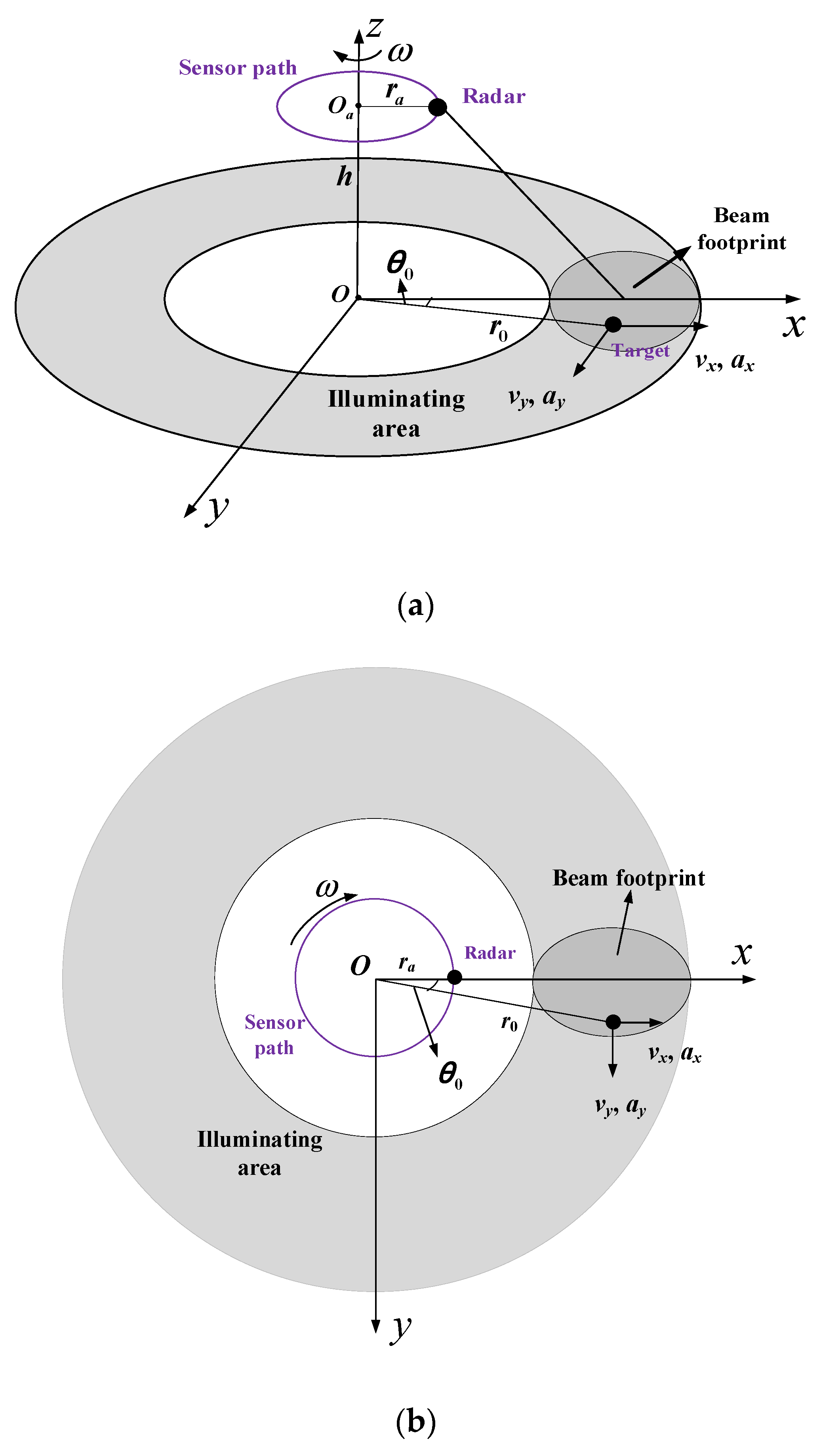
2. Proposed Range Model for CSSAR

2.1. Geometry

The geometric relationship between an airborne CSSAR and a ground moving target is shown in Figure 1. The aircraft travels along a horizonal circle with height h and radius r_a at a constant angular velocity ω, with its antenna pointing perpendicular to the aircraft direction fixedly. At the azimuth slow time t_a = 0, the radar and the target are assumed to be located at (r_a, 0, h) and (r₀ cosθ₀, r₀ sinθ₀, 0), respectively, where r₀ is the distance between the target and the coordinate origin, and θ₀ is the target’s azimuth angle. In addition, it is assumed that the target moves with velocities (v_x, v_y) and constant accelerations (a_x, a_y) along the x-and y-axes.

According to the geometric relationship shown in Figure 1, the instantaneous distance from the radar to the target (i.e., the target’s range equation) can be expressed as

$$R(t_a)=\sqrt{{\left(r_0\cos {\theta }_0+v_x{t}_a+\frac{1}{2}{a}_x{t}_a{}^2-r_a\cos (\omega t_a)\right)}^2+{\left(r_0\sin {\theta }_0+v_y{t}_a+\frac{1}{2}{a}_y{t}_a{}^2-r_a\sin (\omega t_a)\right)}^2+h^2}$$

(1)

Applying Taylor series expansion to (1) around the target’s beam center crossing time, one can obtain

$$R(t_a)=R_c+l_1\left(t_a-t_{ac}\right)+l_2{\left(t_a-t_{ac}\right)}^2++l_3{\left(t_a-t_{ac}\right)}^3+\cdots$$

(2)

With

$$l_1=\frac{v_{tc}(r_c-r_a)}{R_c}$$

(3)

$$l_2=\frac{v_{ta}^2-2r_a\omega \cdot v_{ta}+r_a{r}_c{\omega }^2}{2R_c}+\frac{a_{tc}\left(r_c-r_a\right)}{2R_c}+\frac{h^2{v}_{tc}^2}{2R_c^3}$$

(4)

$$\begin{array}{cc}\hfill l_3& =\frac{v_{ta}\left(a_{tc}+r_a{\omega }^2\right)+a_{ta}\left(v_{tc}-r_a\omega \right)}{2R_c}-\frac{v_{ta}\left(r_c-r_a\right)\left[v_{tc}^2-2v_{tc}{r}_a\omega +v_{ta}^2+r_a{r}_c{\omega }^2+a_{tc}\left(r_c-r_a\right)\right]}{2R_c^3}\hfill \\ & +\frac{v_{ta}^3{\left(r_c-r_a\right)}^3}{2R_c^5}\hfill \end{array}$$

(5)

$$v_{tc}=v_x\cos {\theta }_c+v_y\sin {\theta }_c$$

(6)

$$v_{ta}=v_y\cos {\theta }_c-v_x\sin {\theta }_c$$

(7)

$$a_{tc}=a_x\cos {\theta }_c+a_y\sin {\theta }_c$$

(8)

$$a_{ta}=a_y\cos {\theta }_c-a_x\sin {\theta }_c$$

(9)

where t_ac is the beam center crossing time, R_c is the range between the radar and the target at t_a = t_ac, r_c is the range between the origin of coordinate and the target at t_a = t_ac, v_tc and a_tc are the projections of the target’s velocity and acceleration onto the vertical direction of the radar platform velocity at t_a = t_ac, respectively, and v_ta and a_ta are the projections of the target’s velocity and acceleration onto the direction of the radar platform velocity at t_a = t_ac, respectively, and θ_c is the target’s azimuth angle at t_a = t_ac.

The accuracy of the Taylor-approximated range equation increases with the order of Taylor series expansion. However, when this order is more than two, the derivation of an accurate analytical 2-D spectrum and the design of imaging method will be challenging. Thus, a second-order Taylor expansion is usually applied to the target’s range equation. Nevertheless, when the azimuth resolution goes high or the target moves with accelerations, the accuracy of the second-order Taylor-approximated range equation would be insufficient. Herein, a novel range equation model is proposed. The accuracy of the proposed range model is even higher than that of the third-order Taylor approximated range equation. Moreover, based on the proposed range model, an accurate analytical expression for the target’s 2-D spectrum can be easily derived.

2.2. Proposed Range Model

In order to accomplish an accurate imaging of the target and to allow for an accurate analytical 2-D spectrum to benefit the design of imaging method, the following range equation model is proposed

$$R_p\left(t_a\right)=\sqrt{R_c^2+v_e^2{t}_a^2+\alpha t_a}+\beta t_a$$

(10)

As can be seen from (10), there are three variables (i.e., v_e, α, and β). In order to obtain the expression for these parameters, a third-order Taylor series expansion is applied to (10) and then we obtain

$$R_p\left(t_a\right)\approx R_c+\left(\beta +\frac{\alpha }{2R_c}\right)\left(t_a-t_{ac}\right)+\left(\frac{v_e^2}{2R_c}-\frac{{\alpha }^2}{8R_c^3}\right){\left(t_a-t_{ac}\right)}^2+\left(-\frac{\alpha v_e^2}{4R_c^3}+\frac{{\alpha }^3}{16R_c^5}\right){\left(t_a-t_{ac}\right)}^3$$

(11)

Letting the coefficients of the first, second, and third terms of (11) be equal to those of (2), respectively, one can obtain the expressions for v_e, α, and β as follows

$$v_e=\sqrt{{\left(\frac{R_c{l}_3}{l_2}\right)}^2+2R_c{l}_2}$$

(12)

$$\alpha =-\frac{2R_c^2{l}_3}{l_2}$$

(13)

$$\beta =l_1+\frac{R_c{l}_3}{l_2}$$

(14)

From (10) it can be seen that the proposed range model consists of a hyperbola and a linear term. The proposed range model has two advantages: (1) it allows for an accurate analytical 2-D spectrum which will benefit the design of imaging algorithm (the target’s 2-D spectrum will be presented in the next section); and (2) its accuracy is significantly higher than those of the commonly used second-order and third-order Taylor-approximated range equations.

In the following, the accuracy superiority of the proposed range model over the second-order and third-order Taylor approximated range models are demonstrated via numerical experiments.

The phase error is utilized to indicate the accuracies of the proposed range equation model as well as the second-order and third-order Taylor-approximated range equations, and it is calculated as follows

$$\Omega =\underset{t_a\in \left[-T_a/2,T_a/2\right]}{\max }\left\{4\pi \cdot \frac{\left|R(t_a)-R^{\prime }(t_a)\right|}{\lambda }\right\}$$

(15)

where R(t_a) is the target’s actual range equation, R^′(t_a) indicates the approximated range models (i.e., the proposed range model, the second-order and third-order Taylor approximated range models), λ is the wavelength. T_a is the synthetic aperture time, and it can be approximately expressed as [16]

$$\begin{array}{cc}\hfill T_a& \approx \frac{{\theta }_{bw}{R}_c}{v_g}\hfill \\ & \approx 0.886\cdot \frac{\lambda R_c}{2v_a{\rho }_a}\hfill \end{array}$$

(16)

where θ_bw is the 3 dB beamwidth of the radar, ${\rho }_a\approx 0.886\lambda v_g/(2{\theta }_{bw}{v}_a)$ is the azimuth resolution, v_g = ω·r_c is the velocity of the beam footprint along the ground, and v_a = ω·r_a is the velocity of the radar platform.

In Figure 2 and Figure 3, the phase errors under different velocities and accelerations are illustrated, respectively. The color indicates the value of the phase error with the unit being radian. Comparing Figure 2a with Figure 2b and Figure 3a with Figure 3b, it can be seen that the phase errors of the proposed range model are much smaller than that of the second-order Taylor approximated range equation. Moreover, by comparing Figure 2a with Figure 2c and Figure 3a with Figure 3c, one can see that the phase errors of the proposed range equation model are even smaller than that of the third-order Taylor approximated range equation. These results validate the accuracy superiority of the proposed range equation model over the second-order and third-order Taylor approximated range equations. The parameters of the CSSAR for the simulations are presented in

Table 1. Parameters of airborne CSSAR for simulation.

Parameter	Value
Carrier frequency	10 GHz
Range bandwidth	150 MHz
Sampling frequency	180 MHz
Pulse repetition frequency	1500 Hz
Azimuth resolution	1 m
Illumination time	1.69 s
Flying radius	2.3 km
Platform altitude	8 km
Platform velocity	125 m/s
Ground range of scene center	16 km

.

3. Target’s 2-D Spectrum Based on the Proposed Range Model

After demodulating to the baseband, the target’s signal in the raw data domain can be expressed as

$$s\left(t_r,t_a\right)=w_r\left(t_r-\frac{2R_p\left(t_a\right)}{c}\right)\exp \left\{j\pi k_r{\left[t_r-\frac{2R_p\left(t_a\right)}{c}\right]}^2\right\}\times w_a\left(t_a\right)\exp \left\{-j\pi \frac{4R_p\left(t_a\right)}{\lambda }\right\}$$

(17)

where w_r (·) and w_a (·) denote the range and azimuth envelopes, respectively, t_r is the range time, k_r is the chirp rate of the transmitted signal, c is the speed of light, and f_c is the carrier frequency.

Applying a Fourier transform in range to (17), one can obtain the target’s signal in the range frequency domain as follows

$$S\left(f_r,t_a\right)=W_r\left(f_r\right)\exp \left\{-j\pi \frac{f_r{}^2}{k_r}\right\}\times w_a\left(t_a\right)\exp \left\{-j\pi \frac{4(f_c+f_r)R_P\left(t_a\right)}{c}\right\}$$

(18)

where f_r denotes the range frequency and W_r (·) denotes the range frequency envelope.

To obtain the target’s 2-D spectrum, a Fourier transform in azimuth is applied to (18):

$$S\left(f_r,f_a\right)={\displaystyle {\int }_{-\infty }^{+\infty }S\left(f_r,t_a\right)\exp \left\{-j2\pi f_a{t}_a\right\}d{t}_a}$$

(19)

where f_a denotes the azimuth frequency. To obtain the analytical expression for the target’s 2-D spectrum, the principle of stationary phase [16] is utilized. Based on (10), (18), and (19), the stationary phase point is given by

$$t_a^{*}=-\frac{\sqrt{4v_e^2{R}_c^2-{\alpha }^2}}{2v_e^2}\left[\frac{\left(\frac{c{f}_a}{2v_e(f_c+f_r)}+\frac{\beta }{v_e}\right)}{\sqrt{1-{\left(\frac{c{f}_a}{2v_e(f_c+f_r)}+\frac{\beta }{v_e}\right)}^2}}\right]-\frac{\alpha }{2v_e^2}$$

(20)

According to the principle of stationary phase, the target’s 2-D spectrum can be obtained as follows

$$\begin{array}{cc}\hfill S\left(f_r,f_a\right)& =S\left(f_r,t_a^{*}\right)\exp \left\{-j2\pi f_a{t}_a^{*}\right\}\hfill \\ & =W_r\left(f_r\right)W_a\left(f_a\right)\exp \left\{j\theta (f_r,f_a)\right\}\hfill \end{array}$$

(21)

With

$$\begin{array}{cc}\theta (f_r,f_a)& =-\frac{2\pi \sqrt{4v_e^2{R}_c^2-{\alpha }^2}}{\lambda v_e}\sqrt{1-{\left(\frac{\lambda f_a}{2v_e}+\frac{\beta }{v_e}\right)}^2+\left(1-\frac{\beta }{v_e}\left(\frac{\lambda f_a}{2v_e}+\frac{\beta }{v_e}\right)\right)\left(\frac{2f_r}{f_c}\right)+\left(1-{\left(\frac{\beta }{v_e}\right)}^2\right){\left(\frac{f_r}{f_c}\right)}^2}\\ & +\frac{2\pi \alpha \beta (f_c+f_r)}{c{v}_e^2}+\frac{\pi \alpha f_a}{v_e^2}-\frac{\pi f_r{}^2}{k_r}\hfill \end{array}$$

(22)

where W_a (·) denotes the azimuth frequency envelope.

From the above derivations it can be seen that the analytical expression of the target’s 2-D spectrum can be easily derived without any approximations being made. Therefore, the proposed range model enables the derivation of an accurate analytical expression for the target’s 2-D spectrum.

4. Proposed Imaging Method

In this section, based on the proposed range model and the derived 2-D spectrum of the target, a novel ground moving target imaging method is presented. First, the imaging process is modeled as an optimization problem. Then, the details on utilizing the GA to solve the optimization problem are described. Finally, the flowchart of the proposed imaging method is presented.

4.1. Optimization Modeling

From (21), it can be seen that the target focusing can be accomplished via compensating the phase modulation in the 2-D frequency domain and a 2-D inverse Fourier transform. Based on (21) and (22), the filter for compensating the phase modulation is constructed as follows:

$$H\left(f_r,f_a;v_e,\alpha ,\beta \right)=\exp \left\{\frac{j\pi f_r{}^2}{k_r}+\frac{j2\pi \sqrt{4v_e{}^2{R}_c^2-{\alpha }^2}}{\lambda v_e}\sqrt{\begin{array}{l}1-{\left(\frac{f_a}{2\lambda v_e}+\frac{\beta }{v_e}\right)}^2+\left[1-\frac{\beta }{v_e}\left(\frac{f_a}{2\lambda v_e}+\frac{\beta }{v_e}\right)\right]\left(\frac{2f_r}{f_c}\right)\\ +\left[1-{\left(\frac{\beta }{v_e}\right)}^2\right]{\left(\frac{f_r}{f_c}\right)}^2\end{array}}\right\}$$

(23)

From (23) it can be seen that this filter depends on the three variables of the proposed range model. In practice, these three variables are usually unknown. Therefore, in the process of target imaging, we need to search these variables, and the target will be completely focused when the searched values match the true values of these variables. Given that the contrast of the target’s image will reach its maximum value when the target is completely focused, the process of imaging can be modeled as the following optimization problem

$$\left({\widehat{v}}_e,\widehat{\alpha },\widehat{\beta }\right)=\underset{\begin{array}{l}{v}_{e,t}\in \left[v_{e,\min },v_{e,\max }\right]\\ {\alpha }_t\in [{\alpha }_{\min },{\alpha }_{\max }]\\ {\beta }_t\in [{\beta }_{\min },{\beta }_{\max }]\end{array}}{\arg \max }\left\{\mathrm{Contrast}\left[s\left(t_r,t_a;v_{e,t},{\alpha }_t,{\beta }_t\right)\right]\right\}$$

(24)

With

$$\mathrm{Contrast}\left[s\left(t_r,t_a;v_{e,t},{\alpha }_t,{\beta }_t\right)\right]=\frac{\sqrt{E\left\{{\left[{\left|s\left(t_r,t_a;v_{e,t},{\alpha }_t,{\beta }_t\right)\right|}^2-E\left({\left|s\left(t_r,t_a;v_{e,t},{\alpha }_t,{\beta }_t\right)\right|}^2\right)\right]}^2\right\}}}{E\left\{{\left|s\left(t_r,t_a;v_{e,t},{\alpha }_t,{\beta }_t\right)\right|}^2\right\}}$$

(25)

$$s\left(t_r,t_a;v_{e,t},{\alpha }_t,{\beta }_t\right)={\mathrm{IDFT}}_2\left\{S(f_r,f_a)\cdot H(f_r,f_a;v_{e,t},{\alpha }_t,{\beta }_t)\right\}$$

(26)

where IDFT₂ (·) indicates the 2-D inverse Fourier transform, E (·) presents the spatial average, Contrast (·) is the image contrast, ${\widehat{v}}_e,\widehat{\alpha },\mathrm{and}\widehat{\beta }$ are the estimates of the corresponding variables, v_e,min and v_e,max are the minimum and maximum values of v_e, respectively, α_min and α_max are the minimum and maximum values of α, respectively, and β_min and β_max are the minimum and maximum values of β, respectively.

From the above analysis it can be seen that the solution for the optimization problem is the optimal estimation of the three parameters. Thus, the focused SAR image of the target can be given by

$$I\left(t_r,t_a\right)={\mathrm{IDFT}}_2\left\{S(f_r,f_a)\cdot H(f_r,f_a;{\widehat{v}}_e,\widehat{\alpha },\widehat{\beta })\right\}$$

(27)

If the traditional ergodic search method is utilized to solve the above optimization problem, the computation load will be very high since it is a three-dimensional search. To decrease the computation load, in the following subsection, the GA is used to solve this optimization problem.

4.2. Solving the Optimization Problem via GA

GA starts with encoding the parameters of the search space in the form of a chromosome-like structure. Then, an initial population (a population is constituted by a group of chromosomes) is generated. After that, the fitness value of each individual chromosome of the population is calculated based on a defined fitness function. Subsequently, a selection operation is performed, in which the fittest chromosomes will be chosen with a larger probability. Then, the selected chromosomes are used as parents to produce the next generation by the crossover and mutation operations. This procedure is repeated until the stopping criterion is met.

In this subsection, GA is utilized to solve the optimization problem presented in (24). The specific steps are explained as follows.

(1)

Step 1—Coding: Each individual chromosome of the population is encoded as a binary string with a fixed length. The length of the string depends on the range of the parameters to be searched and the required accuracy. For example, the length of the string for the parameter v_e should be $2^{l_{ve}-1}<(v_{e,\max }-v_{e,\min })/\Delta v_e<2^{l_{ve}}$, where l_ve is the length of the string for v_e, and $\Delta v_e$ is the encoding accuracy for v_e.

(2)

Step 2—Population initialization: The population size NP, the maximum number of generations G_max, and the generation counter g are initialized. All individuals of the population in the 0th generation are generated randomly.

(3)

Step 3—Calculating the fitness: Since the optimization problem is based on maximizing the contrast of the target’s image, the fitness value of a chromosome is chosen to be the contrast of the image that is focused with the parameters corresponding to this chromosome. The image is obtained via (26), and the contrast is calculated via (25).

(4)

Step 4—Selection: The selection operation keeps good chromosomes and eliminates inferior ones. In this paper, to improve the efficiency, the roulette wheel selection rule [33] is adopted, and the selection probability for each chromosome is calculated as follows:

$$p\left({\mathrm{CP}}_{g,n}\right)=\frac{f\left({\mathrm{CP}}_{g,n}\right)}{{\displaystyle \sum _{n=1}^{N}f\left({\mathrm{CP}}_{g,n}\right)}}$$

(28)

where f (·) is the fitness function, and CP_g,n is the nth chromosome of the population in gth generation. In addition, the optimal individual preservation strategy [32] is used. In other words, the optimal individual of the parent population will directly enter the offspring population.

(5)

Step 5—Crossover and mutation: In this paper, the single-point crossover operator and simple mutation operator [33] are applied to the selected chromosomes to produce the population of the next generation.

(6)

Step 6—Judgment: If g is equal to G_max or the maximum fitness value remains stable, jump to step 7. Otherwise, return to step 3.

(7)

Step 7—Output the optimal solution: The chromosome that has the largest fitness value is the optimal solution, and the corresponding parameters are the solutions for the optimization problem. To obtain the solutions for the optimization problem, a decoding operation should be performed with two steps (taking v_e for example): (1) convert the binary string to the decimal number v_e’; (2) calculate the actual value of v_e by (29).

$${\widehat{v}}_e=v_{e,}{}_{\min }+v_e^{\prime }\cdot \frac{v_{e,}{}_{\max }-v_{e,}{}_{\min }}{2^{l_{ve}}-1}$$

(29)

4.3. Flowchart of the Proposed Imaging Method

Based on the analyses presented in Section 4.1 and Section 4.2, the flowchart of the proposed imaging method is presented in Figure 4. It starts with the target signal that has been extracted. First, a 2-D Fourier transform is applied to the target signal to transform the target signal into the 2-D frequency domain. Then, the strategy presented in Section 4.2 is utilized to solve the imaging optimization problem shown in (24). Note that, in using GA to solve the optimization problem, the fitness function is the contrast of the image that is focused with each chromosome, and the image is obtained via (26). Therefore, it is essential to use GA to find the chromosome that obtains the largest image contrast. Finally, with the optimal solution obtained by GA, the target focusing is performed efficiently via (27).

5. Experimental Results

5.1. Validation of the Proposed Range Model

In Section 2.2, we have demonstrated the accuracy superiority of the proposed range model over the second-order and third-order Taylor approximated range models. In this subsection, to further validate the proposed range model, the focusing results based on the original range equation, the proposed range model, the second-order and third-order Taylor-approximated range models are analyzed and compared. The parameters of CSSAR used in the experiments are given in Table 1.

Figure 5 shows the focusing results, with the expanded range and azimuth profiles of the focused target being plotted. In addition, the focusing quality parameters are measured and the results are shown in

Table 2. Measured quality parameters.

		IRW Broadening	PSLR (dB)	ISLR (dB)
Original range model	Azimuth	0.00%	−13.23	−10.12
	Range	0.00%	−13.26	−10.04
Proposed range model	Azimuth	0.00%	−13.12	−9.86
	Range	0.00%	−13.26	−10.04
Second-order Taylor approximated range model	Azimuth	2.03%	−11.05	−9.06
	Range	0.00%	−13.26	−10.04
Third-order Taylor approximated range model	Azimuth	1.35%	−12.91	−9.25
	Range	0.00%	−13.26	−10.04

. The measured quality parameters include the azimuth impulse response width (IRW) broadening, the peak sidelobe ratio (PSLR), and the integrated sidelobe ratio (ISLR) [16]. From Figure 5 and Table 2 it can be seen that the focusing quality of these four range models in range are almost the same. This indicates that the accuracies of these range models are sufficient for range compression and RCM correction. However, it can also be seen that the azimuth profile obtained based on the second-order Taylor approximated range model suffers significant sidelobe asymmetry, IRW broadening, PSLR and ISLR losses. Besides, the focusing result obtained based on the third-order Taylor-approximated range model also suffers azimuth IRW broadening, PSLR and ISLR losses. Nevertheless, quality parameters obtained based on the proposed range model are very close to those obtained based on the original range equation, which indicates that the target is accurately focused.

5.2. Validation of the Proposed Imaging Method

In this subsection, numerical experiments are conducted to investigate the performance of the proposed imaging method. The parameters of CSSAR are given in Table 1. Five moving targets, named T1, T2, T3, T4, and T5, are simulated, and their parameters are presented in

Table 3. Parameters of the moving targets.

	vx (m/s)	vy (m/s)	ax (m/s2)	ay (m/s2)	r0 (km)	θ0 (rad)
T1	−29	20	−0.5	0.3	15.8	0
T2	−5	10	0.1	0.2	15.9	0.01
T3	21	10	−0.4	−0.3	16.0	0
T4	5	−5	0.2	−0.5	16.1	−0.01
T5	−24	−20	0.5	0.4	16.2	0

. The signal-to-noise ratio (SNR) is set to be −10 dB.

In using the GA, first, the value ranges of the parameters to be searched and the encoding accuracies should be determined so that we can encode these parameters. In this paper, it is assumed that v_x∈[−30 m/s, 30 m/s], v_y∈[−30 m/s, 30 m/s], a_x∈[−1 m/s², 1 m/s²], a_y∈[−1 m/s², 1 m/s²]. Then, according to (3)–(9) and (12)–(14), the value ranges of v_e, α, and β can be figured out and the results are: v_e∈[−297.31 m/s, 362.59 m/s], α∈[−7.75 × 10⁵ m²/s, 7.75 × 10⁵ m²/s], β∈[−50.34 m/s, 50.34 m/s]. The encoding accuracies for the three parameters can be set according to the required focusing quality. To keep the azimuth impulse response width (IRW) broadening within 2%, the Doppler chirp rate error should be less than $1/T_a^2$, where T_a is the synthetic aperture time [16]. The Doppler chirp rate is related to v_e and α, and their relationship is as follows

$$K_a=-\frac{4}{\lambda }\left(\frac{v_e^2}{2R_c}-\frac{{\alpha }^2}{8R_c^3}\right)$$

(30)

In the experiments, the bound for the Doppler chirp rate error is set to be $1/(3T_a^2)$. Then, based on (30), the encoding accuracies for v_e and α can be given by (31) and (32), respectively.

$$\Delta v_e=\underset{v_e}{\min }\left\{-v_e+\sqrt{v_e^2+\frac{\lambda R_c}{12T_a^2}}\right\}$$

(31)

$$\Delta \alpha =\underset{\alpha }{\min }\left\{-\alpha +\sqrt{{\alpha }^2+\frac{\lambda R_c^3}{3T_a^2}}\right\}$$

(32)

The derivation for (31) and (32) are presented in Appendix A. As for β, the Doppler center frequency is depended on it and their relationship is formulated in (33). Based on the imaging method shown in (27), the estimation accuracy of β should keep us obtain an accurate Doppler ambiguity. In the simulations, the encoding accuracy for β is given by (34), which could make the estimation error for the Doppler center frequency be less than PRF/10, where PRF is the pulse repetition frequency.

$$f_{ac}=-\frac{2}{\lambda }\left(\beta +\frac{\alpha }{2R_c}\right)$$

(33)

$$\Delta \beta =\lambda \cdot \frac{PRF}{20}$$

(34)

According to (31), (32), and (34), the encoding accuracies for the three parameters are figured out, and the results are: ∆v_e = 0.03 m/s, ∆α = 9000 m²/s, ∆β = 2.25 m/s. In addition, the population size is set to be 50, and the maximum generation is set to be 40. After these parameters being set, the strategy presented in Section 4.2 is utilized to solve the imaging optimization problem. The execution time for each target is measured, which shows that it needs only about 24 min to obtain the optimal solution. The solving processes for the five targets are illustrated in Figure 6, with the optimal image contrasts of each generation being plotted. As can be seen from Figure 6, the proposed method converges quickly.

Figure 7 shows the imaging results, with the contours of target energy being plotted. The results are obtained by extracting a window of 64 × 64 samples centered on the target and then expanding this “window” by a factor of 64 via zero padding the spectrum and inverse transforming. In addition, the image quality parameters are measured and the results are shown in

Table 4. Measured image quality parameters.

		IRW Broadening	PSLR (dB)	ISLR (dB)	Ideal ISLR (dB)
T1	Azimuth	0.81%	−13.21	−10.02	−10.01
	Range	0.00%	−13.16	−9.79	−9.86
T2	Azimuth	0.00%	−13.22	−9.90	−9.96
	Range	0.00%	−13.22	−9.80	−9.86
T3	Azimuth	0.00%	−13.26	−9.98	−10.00
	Range	0.00%	−13.27	−9.88	−9.86
T4	Azimuth	0.00%	−13.25	−9.95	−9.96
	Range	0.00%	−13.22	−9.80	−9.86
T5	Azimuth	0.00%	−13.18	−9.89	−9.94
	Range	0.00%	−13.27	−9.90	−9.86

. The ideal ISLR is measured from the ideal sinc function with the same bandwidth. From Figure 7 it can be seen that the five targets are all finely focused. Moreover, from Table 4 one can see that the image quality parameters are all very close to their theoretical values, which indicates that the targets are accurately focused by the proposed imaging method.

6. Discussions

The experimental results presented in Section 5 validate the proposed range model and the proposed imaging method. In Section 5.1, the qualities of the results obtained based on the original range equation, the proposed range model, the second-order and third-order Taylor-approximated range models are measured and compared. The results demonstrate that the accuracy of the proposed range model is better than that of the second-order and third-order Taylor-approximated range models, and that one can obtain a high-quality focusing result with the proposed range model. In Section 5.2, the imaging results obtained by the proposed method are analyzed. It is seen that the image qualities of the five targets are all close to the theoretical values. Therefore, the proposed imaging method can focus ground moving targets accurately.

The computational load of the proposed imaging method is discussed as follows. According to the analyzes presented in Section 4, the major operations of the proposed method include twice 2-D Fourier transform, twice inverse 2-D Fourier transform, and a 2-D phase multiplication. Assuming that the number of azimuth samples and range samples are N_a and N_r, respectively. Then, the total number of floating operations can be calculated as:

$$20N_r{N}_a{\log }_2(N_r)+20N_r{N}_a{\log }_2(N_a)+6N_r{N}_a$$

(35)

Therefore, the computational order of the proposed method is $O\left(N^2{\log }_{2}N\right)$, where N denotes the 1-D size of the data.

GA is a parallel stochastic algorithm, and it may not converge to the optimal result in a few cases. Now we discuss the variability and statistical significance of the results obtained by GA. Five hundred random experiments are conducted, with the target T1 being considered. The results obtained by these random experiments are analyzed, and the deviations of the obtained optimal image contrasts are plotted in Figure 8. It is found out that there are 479 out of 500 experiments converge to the optimal results. Moreover, it is also figured out that the maximum deviation, the mean deviation, and the standard deviation of the results are 0.1007, 0.0034 and 0.0178, respectively, which are all very small.

7. Conclusions

In this paper, an accurate range model and an efficient ground moving target imaging method have been proposed for airborne CSSAR. The main merits of the proposed range model are highlighted in two aspects: (1) its accuracy is even higher than that of the third-order Taylor approximated range equation; and (2) based on the proposed range model, the accurate analytical expression for the target’s 2-D spectrum can be easily derived. Moreover, an efficient ground moving target imaging method has been proposed. The proposed method focuses the target via a phase multiplication in the 2-D frequency domain and utilizes the GA to accomplish an efficient search of the parameters of the proposed range model. Experimental results have validated the proposed imaging method.

References

1. Moreira, A.; Prats-iraola, P.; Younis, M.; Krieger, G.; Hajnsek, I.P.; Papathanassiou, K. A Tutorial on Synthetic Aperture Radar. IEEE Mag. Geosci. Remote Sens. 2013, 1, 6–43. [Google Scholar] [CrossRef] [Green Version]
2. Jäger, M.; Pinheiro, M.; Ponce, O.; Reigber, A.; Scheiber, R. A Survey of Novel Airborne SAR Signal Processing Techniques and Applications for DLR’s F-SAR Sensor. In Proceedings of the 16th International Radar Symposium (IRS), Dresden, Germany, 24–26 June 2015; pp. 1–6. [Google Scholar]
3. Cantalloube, H.M.J.; Nahum, C.E. Airborne SAR-Efficient Signal Processing for Very High Resolution. Proc. IEEE. 2013, 3, 784–797. [Google Scholar] [CrossRef]
4. Reigber, A.; Scheiber, R.; Jager, M.; Prats-Iraola, P.; Hajnsek, I.; Jagdhuber, T.; Papathanassiou, K.P.; Nannini, M.; Aguilera, E.; Baumgartner, S.; et al. Very-High-Resolution Airborne Synthetic Aperture Radar Imaging: Signal Processing and Applications. Proc. IEEE 2013, 3, 759–783. [Google Scholar] [CrossRef] [Green Version]
5. Ren, Y.; Tang, S.Y.; Guo, P.; So, H.C.; Zhang, L.R. 2-D Spatially Variant Motion Error Compensation for High-Resolution Airborne SAR Based on Range-Doppler Expansion Approach. IEEE Trans. Geosci. Remote Sens. 2021, in press. [Google Scholar] [CrossRef]
6. Jao, J.K. Theory of Synthetic Aperture Radar Imaging of a Moving Target. IEEE Trans. Geosci. Remote Sens. 2001, 9, 1984–1992. [Google Scholar]
7. Bacci, A.; Martorella, M.; Gray, D.A.; Gelli, S.; Berizzi, F. Virtual Multichannel SAR for Ground Moving Target Imaging. IET Radar Sonar Navigat. 2016, 1, 50–62. [Google Scholar] [CrossRef] [Green Version]
8. Zhu, D.Y.; Li, Y.; Zhu, Z.D. A Keystone Transform Without Interpolation for SAR Ground Moving-Target Imaging. IEEE Geosci. Remote Sens. Lett. 2007, 1, 18–22. [Google Scholar] [CrossRef]
9. Wan, J.; Tan, X.; Chen, Z.; Dong, L.; Liu, Q.; Zhou, Y.; Zhang, L. Refocusing of Ground Moving Targets with Doppler Ambiguity Using Keystone Transform and Modified Second-Order Keystone Transform for Synthetic Aperture Radar. Remote Sens. 2021, 2, 177. [Google Scholar] [CrossRef]
10. Zhu, S.Q.; Liao, G.S.; Qu, Y.; Zhou, Z.G.; Liu, X.Y. Ground Moving Targets Imaging Algorithm for Synthetic Aperture Radar. IEEE Trans. Geosci. Remote Sens. 2011, 1, 462–477. [Google Scholar] [CrossRef]
11. Baumgartner, S.V.; Krieger, G. Dual-Platform Large Along-Track Baseline GMTI. IEEE Trans. Geosci. Remote Sens. 2016, 3, 1554–1574. [Google Scholar] [CrossRef]
12. Hashemi, S.R.S.; Bayat, S.; Nayebi, M.M. Ground-Based Moving Target Imaging in a Circular Strip-Map Synthetic Aperture Radar. In Proceedings of the IEEE 5th Asia-Pacific Conference on Synthetic Aperture Radar (APSAR), Singapore, 1–4 October 2015; pp. 835–840. [Google Scholar]
13. Shao, Y.; Chen, Z.Y.; Wu, X.B. Investigation on Imaging Performance of Circular Scanning Synthetic Aperture Radar. In Proceedings of the XXXIth URSI General Assembly and Scientific Symposium (URSI GASS), Beijing, China, 16–23 August 2014; pp. 1–4. [Google Scholar]
14. Liao, Y.; Wang, W.Q.; Liu, Q.H. Two-Dimensional Spectrum for Circular Trace Scanning SAR Based on an Implicit Function. IEEE Geosci. Remote Sens. Lett. 2016, 7, 887–891. [Google Scholar] [CrossRef]
15. Baumgartner, S.V. Circular and Polarimetric ISAR Imaging of Ships Using Airborne SAR Sensors. In Proceedings of the 12th European Conference on Synthetic Aperture Radar (EUSAR), Berlin, Germany, 4–7 June 2018; pp. 1–6. [Google Scholar]
16. Cumming, I.G.; Wong, F.H. Digital Processing of Synthetic Aperture Radar Data: Algorithm and Implementation; Artech House: Norwood, MA, USA, 2004. [Google Scholar]
17. Sun, G.C.; Xing, M.D.; Xia, X.G.; Wu, Y.R.; Bao, Z. Robust Ground Moving-Target Imaging Using Deramp–Keystone Processing. IEEE Trans. Geosci. Remote Sens. 2013, 2, 966–982. [Google Scholar] [CrossRef]
18. Wang, G.Y.; Xia, X.G.; Chen, V.C. Dual-Speed SAR Imaging of Moving Targets. IEEE Trans. Aerosp. Electron. Syst. 2006, 1, 368–379. [Google Scholar] [CrossRef]
19. Noviello, C.; Fornaro, G.; Martorella, M. Focused SAR Image Formation of Moving Targets Based on Doppler Parameter Estimation. IEEE Trans. Geosci. Remote Sens. 2015, 2, 966–982. [Google Scholar] [CrossRef]
20. Baumgartner, S.V.; Krieger, G. Multi-Channel SAR for ground Moving Target Indication. Elsevier Acad. Press Libr. Signal Process. 2014, 2, 911–986. [Google Scholar]
21. Zhang, X.P.; Liao, G.S.; Zhu, S.Q.; Zeng, C.; Shu, Y.X. Geometry-Information-Aided Efficient Radial Velocity Estimation for Moving Target Imaging and Location Based on Radon Transform. IEEE Trans. Geosci. Remote Sens. 2015, 2, 1105–1117. [Google Scholar] [CrossRef]
22. Huang, P.H.; Liao, G.S.; Yang, Z.; Xia, X.G.; Ma, J.T.; Zheng, J.B. Ground Maneuvering Target Imaging and High-Order Motion Parameter Estimation Based on Second-Order Keystone and Generalized Hough-HAF Transform. IEEE Trans. Geosci. Remote Sens. 2017, 1, 320–335. [Google Scholar] [CrossRef]
23. Zeng, C.; Li, D.; Luo, X.; Liu, H.Q.; Su, J. Ground Maneuvering Targets Imaging for Synthetic Aperture Radar Based on Second-Order Keystone Transform and High-Order Motion Parameter Estimation. IEEE J. Sel. Topics Appl. Earth Observ. Remote Sens. 2019, 11, 4486–4501. [Google Scholar] [CrossRef]
24. Li, D.; Ma, H.N.; Liu, H.Q.; Chen, Z.Y.; Su, J.; Zhou, X.C.; Li, W.; Yang, Z.J. An Efficient Ground Maneuvering Target Refocusing Method Based on Principal Component Analysis and Motion Parameter Estimation. Remote Sens. 2020, 12, 1–22. [Google Scholar] [CrossRef]
25. Huang, L.J.; Qiu, X.; Hu, D.; Ding, C. Focusing of Medium-Earth-Orbit SAR with Advanced Nonlinear Chirp Scaling Algorithm. IEEE Trans. Geosci. Remote Sens. 2011, 49, 500–508. [Google Scholar] [CrossRef]
26. Li, Y.K.; Wang, T.; Liu, B.C.; Hu, R.X. High-Resolution SAR Imaging of Ground Moving Targets Based on the Equivalent Range Equation. IEEE Geosci. Remote Sens. Lett. 2015, 2, 324–328. [Google Scholar]
27. Zhang, Y.; Sun, J.P.; Lei, P.; Li, G.; Hong, W. High-Resolution SAR-Based Ground Moving Target Imaging With Defocused ROI Data. IEEE Trans. Geosci. Remote Sens. 2016, 2, 1062–1073. [Google Scholar] [CrossRef]
28. Jin, G.H.; Dong, Z.; He, F.; Yu, A.X. SAR Ground Moving Target Imaging Based on a New Range Model Using a Modified Keystone Transform. IEEE Trans. Geosci. Remote Sens. 2019, 6, 3283–3295. [Google Scholar] [CrossRef]
29. Jao, J.K.; Yegulalp, A. Multichannel Synthetic Aperture Radar Signatures and Imaging of a Moving Target. Inverse Probl. 2013, 5, 1–33. [Google Scholar] [CrossRef]
30. Yang, J.; Liu, C.; Wang, Y.F. Imaging and Parameter Estimation of Fast-Moving Targets with Single-Antenna SAR. IEEE Geosci. Remote Sens. Lett. 2014, 2, 529–533. [Google Scholar] [CrossRef]
31. Yang, L.; Zhao, L.F.; Bi, G.A.; Zhang, L.R. SAR Ground Moving Target Imaging Algorithm Based on Parametric and Dynamic Sparse Bayesian Learning. IEEE Trans. Geosci. Remote Sens. 2016, 4, 2254–2267. [Google Scholar] [CrossRef]
32. Srinivas, M.; Patnaik, L.M. Genetic Algorithms: A Survey. Computer 1994, 6, 17–26. [Google Scholar] [CrossRef]
33. Whitley, D. A Genetic Algorithm Tutorial. Stattics Comput. 1994, 4, 65–85. [Google Scholar] [CrossRef]
34. Zhang, J.; Chung, H.S.H.; Lo, W.L. Clustering-Based Adaptive Crossover and Mutation Probabilities for Genetic Algorithms. IEEE Trans. Evol. Comput. 2007, 3, 326–335. [Google Scholar] [CrossRef]
35. Chen, Y.J.; Zhang, Q.; Luo, Y.; Chen, Y.A. Measurement Matrix Optimization for ISAR Sparse Imaging Based on Genetic Algorithm. IEEE Trans. Geosci. Remote Sens. 2016, 12, 1875–1879. [Google Scholar] [CrossRef]
36. Shi, L.; Deng, Y.K.; Sun, H.F.; Wang, R.; Ai, J.Q.; Yan, H. An Improved Real-Coded Genetic Algorithm for the Beam Forming of Spaceborne SAR. IEEE Trans. Antennas Propag. 2012, 6, 3034–3040. [Google Scholar] [CrossRef]
37. Zhang, T.; Liao, G.S.; Li, Y.C.; Gu, T.; Zhang, T.H.; Liu, Y.J. A Two-Stage Time-Domain Autofocus Method Based on Generalized Sharpness Metrics and AFBP. IEEE Trans. Geosci. Remote Sens. 2021, in press. [Google Scholar] [CrossRef]
Figure 1. Geometry of airborne CSSAR. (a) 3-D view and (b) top view.
Remotesensing 14 00210 g001
Figure 2. Phase errors under different velocities. (a) Proposed range equation, (b) second-order Taylor approximated range equation, and (c) third-order Taylor approximated range equation. The parameters of the target are: Rc = 20 km, ax = 0.3 m/s2, and ay = 0.2 m/s2.
Remotesensing 14 00210 g002
Figure 3. Phase errors under different accelerations. (a) Proposed range equation, (b) second-order Taylor approximated range equation, and (c) third-order Taylor approximated range equation. The parameters of the target are: Rc = 20 km, vx = 5 m/s, and vy = 13 m/s.
Remotesensing 14 00210 g003
Figure 4. Flowchart of the proposed imaging method.
Remotesensing 14 00210 g004
Figure 5. Focusing results. (a) azimuth profile, (b) range profile. The parameters of the target are Rc = 21 km, vx = 3 m/s, vy = −12 m/s, ax = 0.6 m/s2 and ay = −0.3 m/s2.
Remotesensing 14 00210 g005
Figure 6. Solving processes of the optimization problem. (a) T1, (b) T2, (c) T3, (d) T4, and (e) T5.
Remotesensing 14 00210 g006aRemotesensing 14 00210 g006b
Figure 7. Contour plots of the five targets. (a) T1, (b) T2, (c) T3, (d) T4, and (e) T5.
Remotesensing 14 00210 g007aRemotesensing 14 00210 g007b
Figure 8. Deviations of the optimal image contrasts obtained by 500 random experiments.
Remotesensing 14 00210 g008