Parameter Estimation for Sea Clutter Pareto Distribution Model Based on Variable Interval

Abstract

The generalized Pareto (GP) distribution model is often used to describe the amplitude statistical feature of sea clutter. Generally, the parameters of GP distribution are estimated by moments estimators. However, when the sea state is high, the appearance of sea spikes will increase the echo of the anomalous scattering units, which leads to a decrease in the parameter estimation accuracy and target detection performance. To improve the parameter estimation accuracy, this paper proposes a novel parameter estimation method based on variable intervals. Considering the local properties of sea clutter, we take a variable interval of the entire sea clutter series for parameter estimation, where the interval position is selected according to the sea state conditions. For contrast, the bipercentile parameter estimation and truncate moment estimation are also introduced. Finally, the experiment based on the real measured X-band sea clutter datasets indicates that the proposed method outperforms the state-of-the-art moments estimators.

1. Introduction

Sea clutter is the backscattered interference signal from the sea surface. In the field of radar target detection under a sea background, maritime radar usually faces interference from heavy sea clutter echoes, which severely restrict the radar target detection performance [1,2]. Among the complex properties of sea clutter, the probability density function (PDF) of the sea clutter amplitude distribution model is the theoretical basis for designing the constant false alarm rate (CFAR) detector [3]. In order to improve the target detection performance, the sea clutter model needs to be accurately matched, and the model parameters should be accurately estimated. In the past few years, plenty of sea clutter distribution models have been investigated, such as Rayleigh distribution, Weibull distribution, Log-normal distribution and K-distribution [4,5,6,7,8,9]. However, due to sea clutter not only being affected by natural environmental factors such as wind speed, wind direction, and sea conditions but also by frequency, incident angle, signal bandwidth and other radar working parameters [10], sea clutter usually presents temporal–spatial correlations and non-Gaussian properties [11], of which the sea clutter is often described by K-distribution with Gamma-distributed textures [12]. However, with the development of radar technology, radar resolution has been improved continuously, and the K-distribution fitting performance of the sea clutter tail part is degraded under low glancing angle. To overcome the shortcomings above, the generalized Pareto (GP) distribution model with inverse Gamma texture is proposed [13,14,15,16], which not only considers the temporal–spatial correlations and tailing characteristics of sea clutter, but also has a relatively simple probability density function expression. Therefore, the GP model is widely used in sea clutter modeling and target detection field [17,18,19,20,21,22], and it is important to research accurate parameter estimation methods for GP distribution.

The most commonly used parameter estimations are maximum likelihood (ML) estimator and moments (MoM) estimators [23,24,25]. In general, since the accuracy of parameters of the ML estimator is higher than the MoM estimator, the ML estimator is preferred for parameter estimation such as Rayleigh distribution, Weibull distribution and Log-normal distribution. However, due to the computational complexity of ML estimators being higher than MoM estimators, it is difficult to use ML estimators to estimate the parameters of K distribution and GP distribution with a compound model. Therefore, the parameter estimation method of the GP distribution is mainly based on the MoM estimator [26,27,28]. However, the traditional MoM estimator only considers the entire sea clutter amplitude series and ignores the local properties of the sea clutter. When the sea state is high, with the appearance of sea spikes, the measured sea clutter data usually contain anomalous scattering units with a strong power value, which leads to a decrease in the performance of the MoM estimator. Moreover, the MoM estimators may be invalid when the value of the shape parameter dissatisfies the restricted conditions [29,30].

To overcome the shortcomings of the MoM estimators, the authors of [31] constructed the bipercentile (BiP) parameter estimation method. However, only a set of biquantiles is used to perform parameter estimation in the BiP method, which leads to a decrease in the stability of parameter estimation. In order to enhance the stability of parameter estimation, the truncated moment estimation was proposed in reference [32]. The main idea of truncated moment estimation is to combine quantile information and moment estimation. However, the truncated moment estimation is unable to adjust the initial position of sea clutter sequence for parameter estimation according to sea state.

In order to further decrease the influence of sea spikes for parameter estimation and enhance the accuracy of parameter estimation, this paper proposes a novel parameter estimation method based on the local statistical properties of sea clutter amplitude sequence. The proposed method is an improvement on the MoM estimation estimators, which focus on the local properties of sea clutter. The proposed method takes the sea clutter data in a special interval for parameter estimation, and the interval position is selected according to the sea state, which can adapt to different maritime radar working environments. When the sea state is high, the larger amplitude sea clutter sequences are dominant, and the interval position is selected in the middle and tail part of the sorted series. Likewise, when the sea state is low, the interval position is selected in the front and middle part of the sorted series. Then, the zero-moment is also constructed as a part of the parameter estimator, which increases the parameter estimation accuracy. Through analysis of real and simulated sea clutter datasets, the results show that the proposed method can increase the accuracy of the parameter estimation for GP model.

The remainder of this paper is organized as follows. Section 2 introduces the PDF of the GP Distribution and the MoM, BiP and truncated moment estimators. Then, the variable interval estimation (VIE) method is proposed, while the algorithm procedures are discussed in detail. Section 3 accomplishes the VIE of GP distribution based on the measured and simulated sea clutter data and analyzes the parameter estimation performance. Section 4 summarizes the full text.

2. Method

In this section, the PDF of the GP distribution is first introduced. Then, in order to testify the effectiveness of the proposed method, the MoM, BiP parameter estimation [19] and truncated moment estimation [20] are derived. At last, the proposed VIE is discussed in detail, and the common goodness of fit test (GOF) methods are also introduced briefly.

2.1. The PDF of the GP Distribution

The GP distribution is a compound Gaussian distribution model, which is a production of the fast changing speckle component and the slow changing structural component. The reception vector of the GP distribution is expressed as:

$$c=\sqrt{\tau }u$$

(1)

where c is the reception vector, u is the rapidly varying speckle component, and τ is a slowly varying texture component. Moreover, the speckle component u obeys a complex Gaussian random variable with a mean value of 0, while the slowly varying texture component τ is a random variable subject to inverse gamma distribution. The PDF of inverse gamma distribution is expressed as follows:

$$f\left(\tau \right)={\left(\frac{\lambda }{a}\right)}^{\lambda }\frac{{\tau }^{-\lambda -1}}{\mathrm{\Gamma }\left(\lambda \right)}\exp \left(-\frac{\lambda }{a\tau }\right)$$

(2)

where $a$ is the scale parameter, $\lambda$ is the shape parameter of inverse gamma distribution, and $\mathrm{\Gamma }\left(\cdot \right)$ is the gamma function. The magnitude of the sea clutter vector can be expressed as:

$$x\left(i\right)=\left|c\left(i\right)\right|=\left|\sqrt{\tau \left(i\right)}u\left(i\right)\right|$$

(3)

where $c\left(i\right)$ is the i-th component of the sea clutter vector. When the texture component $\tau \left(i\right)$ is known, the clutter amplitude $x\left(i\right)$ obeys the Rayleigh distribution. The expression of the conditional PDF of the clutter amplitude $x\left(i\right)$ is:

$$f\left(x|\tau \right)=\frac{2x}{\tau }\exp \left(-\frac{x^2}{\tau }\right)$$

(4)

According to the total probability theorem, the PDF of the GP distribution is deduced as follows, which is equal to the definition of the square root of the Pareto distribution [6]:

$$f\left(x\right)=\frac{2ax}{{\left(a{\lambda }^{-1}{x}^2+1\right)}^{\lambda +1}}$$

(5)

where $x$ represents the sea clutter amplitude, $a$ represents the scale parameter, and $\lambda$ represents the shape parameter, which determines the non-Gaussian nature of sea clutter. The shape parameter $\lambda$ decides the tail length of the PDF. When $\lambda \to \infty$, the GP distribution degenerates to the Rayleigh distribution, and the GP distribution has a shorter tail. When $\lambda \to 0$, the GP distribution has a heavier tail. The scale parameter $a$ decides the average power of the sea clutter. When the value of scale parameter $a$ increases, the average power of the sea clutter will decrease.

2.2. The MoM of GP Distribution

The methods of the MoM estimator and ML estimator are used to estimate parameters of the sea clutter model. Due to the computational burden of ML methods, the ML estimator is unsuitable to estimate the GP distribution parameters. Therefore, the estimator-based MoM is taken to estimate the GP distribution parameters, which have less computational cost.

According to the PDF of the GP distribution and the principle of the MoM method, the k-th moment of GP is calculated as (6):

$$E\left(X^k\right)=2a{\displaystyle \underset{0}{\overset{\infty }{\mathrm{\int }}}\frac{x^{k+1}}{{\left(a{\lambda }^{-1}{x}^2+1\right)}^{\lambda +1}}}dx$$

(6)

where $X^k$ represents the k order origin moment of the sea clutter amplitude sequence. Substituting $r=\frac{a}{\lambda }{x}^2$ into (6), the following expression can be obtained.

$$E\left(X^k\right)={\left(\frac{\lambda }{a}\right)}^{k/2}\lambda {\displaystyle \underset{0}{\overset{\infty }{\mathrm{\int }}}\frac{r^{k/2}}{{\left(r+1\right)}^{\lambda +1}}}dr$$

(7)

According to the definition of the Beta function ${\displaystyle \underset{0}{\overset{\infty }{\int }}{t}^{z-1}}/{\left(1+t\right)}^{z+w}dt=\mathrm{\Gamma }\left(z\right)\mathrm{\Gamma }\left(w\right)/\mathrm{\Gamma }\left(z+w\right)$ and the property of the Gamma function $\mathrm{\Gamma }\left(z+1\right)=z\mathrm{\Gamma }\left(z\right)$, the k-th MoM estimator of the GP distribution is defined as (8):

$$E\left(X^k\right)={\left(\frac{\lambda }{a}\right)}^{k/2}\frac{\mathrm{\Gamma }\left(1+k/2\right)\mathrm{\Gamma }\left(\lambda -k/2\right)}{\mathrm{\Gamma }\left(\lambda \right)}$$

(8)

When $\lambda >k/2$, Formula (8) is valid. Then, the half and one moments estimation are selected to obtain the GP distribution parameters, which is expressed as (9):

$$\left\{\begin{array}{c}E\left(X^{\frac{1}{2}}\right)={\left(\frac{\lambda }{a}\right)}^{1/2}\frac{\mathrm{\Gamma }\left(3/2\right)\mathrm{\Gamma }\left(\lambda -1/2\right)}{\mathrm{\Gamma }\left(\lambda \right)}\\ E\left(X^{\frac{1}{4}}\right)={\left(\frac{\lambda }{a}\right)}^{1/4}\frac{\mathrm{\Gamma }\left(5/4\right)\mathrm{\Gamma }\left(\lambda -1/4\right)}{\mathrm{\Gamma }\left(\lambda \right)}\end{array}\right.$$

(9)

2.3. BiP Parameter Estimation

There are plenty of sea spikes in the sea clutter sequence, and sea spikes will cause a decrease in the accuracy of MoM. Moreover, when we use the MoM estimator to estimate the parameters of GP distribution, the shape parameter λ must satisfy restricted conditions. In order to solve the problems above, the BiP is proposed. The specific algorithm of BiP is shown as follows.

According to the PDF of the GP distribution, the cumulative distribution function (CDF) of GP distribution can be derived as (10):

$$F\left(x\right)=P\left(\tau <x\right)={\displaystyle \underset{0}{\overset{x}{\int }}f\left(\tau \right)}d\tau =1-{\left(1+a{\lambda }^{-1}{x}^2\right)}^{-\lambda }$$

(10)

where $P\left(A\right)$ represents the probability of the appearance of A. Next, we define the conception of quantile point as follows:

$$\alpha =P\left(x\le x_{\alpha }\right)=F\left(x_{\alpha }\right)$$

(11)

where $\alpha$ represents an arbitrary quantile point and $0<\alpha <1$, $x_{\alpha }$ represents this quantile point correspond to the value of amplitude of sorted sample sequence. Then, substitute the CDF of GP distribution into (11), and we can obtain an equation as follows:

$${\left(1+a{\lambda }^{-1}{x}_{\alpha }\right)}^{\lambda }\left(1-\alpha \right)=1$$

(12)

Therefore, we can utilize arbitrary bipercentile ${\alpha }_1$ and ${\alpha }_2$ to obtain an equation set to estimate the parameters. The equation set can be expressed as follows:

$$\left\{\begin{array}{c}{\left(1+a{\lambda }^{-1}{x}_{{\alpha }_1}\right)}^{\lambda }\left(1-{\alpha }_1\right)=1\\ {\left(1+a{\lambda }^{-1}{x}_{{\alpha }_2}\right)}^{\lambda }\left(1-{\alpha }_2\right)=1\end{array}\right.$$

(13)

2.4. Truncated Moment Estimation

Since the BiP method only uses a pair of quantile points in a sea clutter series to perform parameter estimation, which severely affects stability of parameter estimation. To overcome this defect, the truncated moment estimation is proposed, and the specific algorithm of the truncated moment estimation is inferred as follows.

According to the quantile point $\alpha$ and the PDF of the GP distribution, the second truncated moment is defined as follows.

$$m_{2,\alpha }={\displaystyle \underset{0}{\overset{x_{\alpha }}{\int }}{x}^{2}f\left(x\right)}dx$$

(14)

Substitute the PDF of the GP distribution into (14), and the truncated moment estimation can be simplified as follows.

$$m_{2,\alpha }=\frac{\lambda }{a\left(\lambda -1\right)}\left(1-{\left(\frac{1}{1+a{\lambda }^{-1}{x}_{\alpha }{}^2}\right)}^{\lambda -1}\right)-z_{\alpha }{}^2{\left(\frac{1}{1+a{\lambda }^{-1}{x}_{\alpha }{}^2}\right)}^{\lambda }$$

(15)

Moreover, when we use the quantile $\alpha$, the Formula (12) is sure to exist. Therefore, we can simultaneously utilize Equations (12) and (15) to estimate the parameters of GP distribution, and the equation set can be shown as follows.

$$\left\{\begin{array}{l}{m}_{2,\alpha }=\frac{\lambda }{a\left(\lambda -1\right)}\left(1-{\left(\frac{1}{1+a{\lambda }^{-1}{x}_{\alpha }{}^2}\right)}^{\lambda -1}\right)-z_{\alpha }{}^2{\left(\frac{1}{1+a{\lambda }^{-1}{x}_{\alpha }{}^2}\right)}^{\lambda }\hfill \\ x_{\alpha }=\sqrt{\frac{\lambda }{a}\left[\exp \left(-\frac{\ln \left(1-\alpha \right)}{\lambda }\right)-1\right]}\hfill \end{array}\right.$$

(16)

2.5. The VIE Method

It is known that the statistical property of sea clutter varies with the changing of sea state. In order to further enhance the accuracy of parameter estimation, this paper proposed a novel parameter estimation method based on the variable interval, where the sea clutter interval for parameter estimation is chosen based on sea state. The detailed processing of the VIE method is discussed as follows.

Radar echo acquisition and preprocessing. Suppose that $X=\{x_{\left(k\right)},k=1,2,3\dots N\}$ represents the original radar sea clutter time sequence. Then, sea clutter time sequence $X$ is sorted in order from smallest to largest, which is expressed as:

$$X=\left\{x_{\left(k\right)},k=1,2,3\dots N\right\}$$

(17)

Variable interval location selection. Rather than estimating the distribution parameters based on the whole sea clutter sample, only the samples in the selected interval are taken for parameter estimation. The criterion for the interval position selection is discussed as follows. First, the percentile l₁, l₂ is defined as follows.

$$\left\{l_1,l_2|0<l_1<l_2<1\right\}$$

(18)

Suppose the length of sea clutter series is N, and the interval position is L₁, L₂, which are corresponding with l₁, l₂, then the corresponding relationship between l₁, l₂ and L₁, L₂ is shown as follows.

$$\left\{\begin{array}{c}{\widehat{x}}_{\left(L1\right)}=x_{\left(N{l}_1\right)}\\ {\widehat{x}}_{\left(L_2\right)}=x_{\left(N{l}_2\right)}\end{array}\right.$$

(19)

where ${\widehat{x}}_{\left(L_1\right)}$ and ${\widehat{x}}_{\left(L_2\right)}$ represent the starting and ending of sea clutter sequences in the interval, respectively. The criterion for choosing the interval location is mainly according to the sea state. When the sea state is less than 2, the sea surface is calm and the small amplitude sea clutter sequences are dominant. In this condition, the interval is selected in the front and middle part of the sea clutter amplitude series X. When the sea state is more than 3, sea spikes emerge and the large amplitude sea clutter sequences are dominant. In this condition, the interval should be selected in the middle and tail part, which can obtain a more exactly parameter estimation result of the tail part. Moreover, when the sea state is near 3, the interval can be selected in the middle part. The sketch map of the interval location selection is shown in Figure 1.

In practice, the selections of interval location are also based on the sea state. According to the sea state, the interval locations for parameter estimation can be preliminarily selected. Then, the locations of the interval are slightly adjusted by searching the superior interval based on the GOF results.

The sea clutter series in the interval can be defined as:

$$X^{\prime }=\left\{x_{\left(L_1\right)},x_{\left(L_1+1\right)},\dots ,x_{\left(L_2-1\right)},x_{\left(L_2\right)}\right\}$$

(20)

Parameter estimation based on variable interval. First, according to the PDF of the GP distribution, the second-order interval moment is calculated as follows.

$$m_{2,x_{\left(L_1\right)},x_{\left(L_2\right)}}={\displaystyle \underset{{\widehat{x}}_{\left(L_1\right)}}{\overset{{\widehat{x}}_{\left(L_2\right)}}{\int }}{x}^{2}f\left(x\right)}dx$$

(21)

Then, the mean square of the sea clutter series in the interval is calculated as follows.

$${\widehat{m}}_{2,x_{\left(L_1\right)},x_{\left(L_2\right)}}=\frac{1}{N}{\displaystyle \sum _{i=x_{\left(L_1\right)}}^{x_{\left(L_2\right)}}{x}_i^2}$$

(22)

Since there are two GP parameters to be estimated, it is necessary to construct two equations to calculate the parameters. The half and one MoM method takes the first-order moment as the second equation for parameter estimation. To increase the parameter estimation accuracy, the zero-order interval moment is constructed to estimate the parameters. The essence for calculating the zero-order moment is to compute the percentage of the sea clutter sequence $X^{\prime }$ in the interval to the entire sequence $X$. According to the PDF of the GP distribution, the zero-order interval moment is calculated as follows.

$$w_{x_{\left(L_1\right)},x_{\left(L_2\right)}}={\displaystyle \underset{x_{\left(L_1\right)}}{\overset{x_{\left(L_2\right)}}{\int }}f\left(x\right)}dx=l_2-l_1$$

(23)

where $w_{x_{\left(L_1\right)},x_{\left(L_2\right)}}$ represents the zero-order moment of the theoretical value and l₁ − l₂ represents the zero-order moment of estimated value.

Finally, according to (20)–(22), the second-order and zero-order moments are combined to estimate the GP parameters, which are shown as follows.

$$\left\{\begin{array}{l}{m}_{\mathrm{2,}{x}_{\left(L_1\right)},x_{\left(L_2\right)}}={\widehat{m}}_{\mathrm{2,}{x}_{\left(L_1\right)},x_{\left(L_2\right)}}\hfill \\ w_{x_{\left(L_1\right)},x_{\left(L_2\right)}}=l_1-l_2\hfill \end{array}\right.$$

(24)

Substituting the measured sea clutter data X′ and PDF of the GP distribution into (24), the following equation can be obtained.

$$\left\{\begin{array}{l}\frac{a\lambda \left(x_{\left(L_2\right)}{}^2-x_{\left(L_1\right)}{}^2\right)+\lambda -{\lambda }^2}{a\left(\lambda -1\right)}\left(l_2-l_1\right)=\frac{1}{N}{\displaystyle \sum _{i=x_{\left(L_1\right)}}^{x_{\left(L_2\right)}}{x}_i^2}\hfill \\ {\left(1+a{\lambda }^{-1}{x}_{\left(L_1\right)}{}^2\right)}^{-\lambda }-{\left(1+a{\lambda }^{-1}{x}_{\left(L_2\right)}{}^2\right)}^{-\lambda }=l_2-l_1\hfill \end{array}\right.$$

(25)

Then, the parameters $a$ and $\lambda$ are obtained by solving (25).

2.6. Histogram Statistics and GOF Test

After counting the histogram of the sea clutter series, the fit errors between the histogram statistics of the sea clutter amplitude series and fitted distribution model are analyzed. Then, the mean square difference (MSD), the Kolmogorov–Smirnov (K-S) distance, and the modified mean square difference (MMSD) methods are taken to evaluate the consequent of the GOF test. MSD and K-S distance are used to test the fitting effect of the entire fit model, MMSD focuses on testing the fitting effect of the tail of the fit model.

(1)

The calculation of MSD is defined as:

$$D_{msd}=\frac{1}{N}{{\displaystyle \sum _{k=1}^N\left(f_r\left(x_k\right)-f_t\left(x_k\right)\right)}}^2$$

(26)

where $f_r\left(·\right)$ represents the frequency of sea clutter sequence in histogram, $f_t\left(·\right)$ represents the PDF of fit model, k represents the sequence number of the sea clutter sequence, N represents the length of sea clutter sequence.

(2)

The calculation of K-S distance is defined as:

$$KSD=\max \left(\left|F_0\left(x\right)-F_N\left(x\right)\right|\right)$$

(27)

where KSD represents the K-S distance, $F_0\left(x\right)$ represents the CDF of the fit model, and $F_N\left(x\right)$ represents the empirical CDF of the sample sequence.

(3)

The calculation of MMSD is defined as:

$$\begin{gathered} D_{mmsd}=\frac{1}{M}{{\displaystyle \sum _{k_{tail}=1}^M\left(f_r\left(x_{k_{tail}}\right)-f_t\left(x_{k_{tail}}\right)\right)}}^2 \\ \left\{x_{k_{tail}}|k_{tail}=1,2,\cdots ,M;1-F_r\left(x_{k_{tail}}\right)\le P_f\right\} \end{gathered}$$

(28)

where the definition of $f_r\left(·\right)$ and $f_k\left(·\right)$ are same as MSD, $x_{k_{tail}}$ represents the sample aggregation of tail. If the smallest $x_{k_{tail}}$ is the detection threshold, the function $1-F_r\left(x_{k_{tail}}\right)\le P_f$ is CFAR detection, $P_f$ is the false alarm probability.

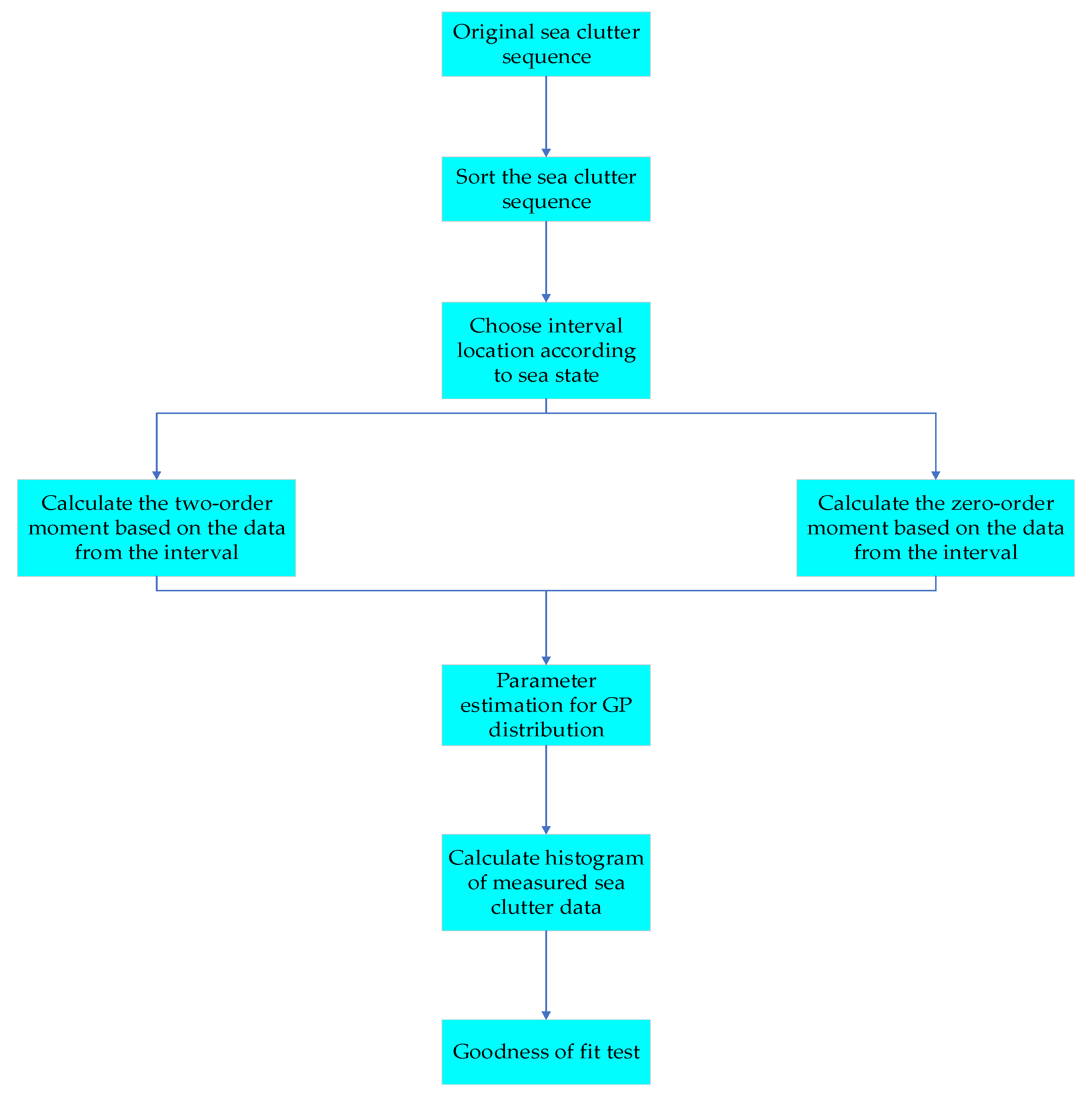
Moreover, the flow chart of the proposed parameter estimation method is shown in Figure 2.

The proposed parameter estimation method is presented in Figure 2 and can be summarized as follows:

• Step 1: Radar echo acquisition and preprocessing. Sort the original sea clutter time sequence according to the criterion from smallest to largest and obtain the sorted sea clutter sequence $X$.
• Step 2: Variable interval location selection. Select the sea clutter data form the sorted sea clutter sequence $X$ based on the sea state.
• Step 3: Parameter estimation for GP distribution. Calculate the one-order and two-order moments based on the data from interval and estimate the parameters of GP distribution through simultaneous equations.
• Step 4: Goodness of fit test. Calculate the fit errors between the histogram of measured sea clutter data and the fit model based on the MSD, K-S distance and MMSD algorithm.

3. Results and Discussion

In this section, the real measured X-band sea clutter data are taken to analyze the performance of the proposed parameter estimation method. Moreover, the Monte Carlo experiments are also performed to enhance the persuasiveness of the proposed method.

3.1. Real Sea Clutter Datasets Introduction

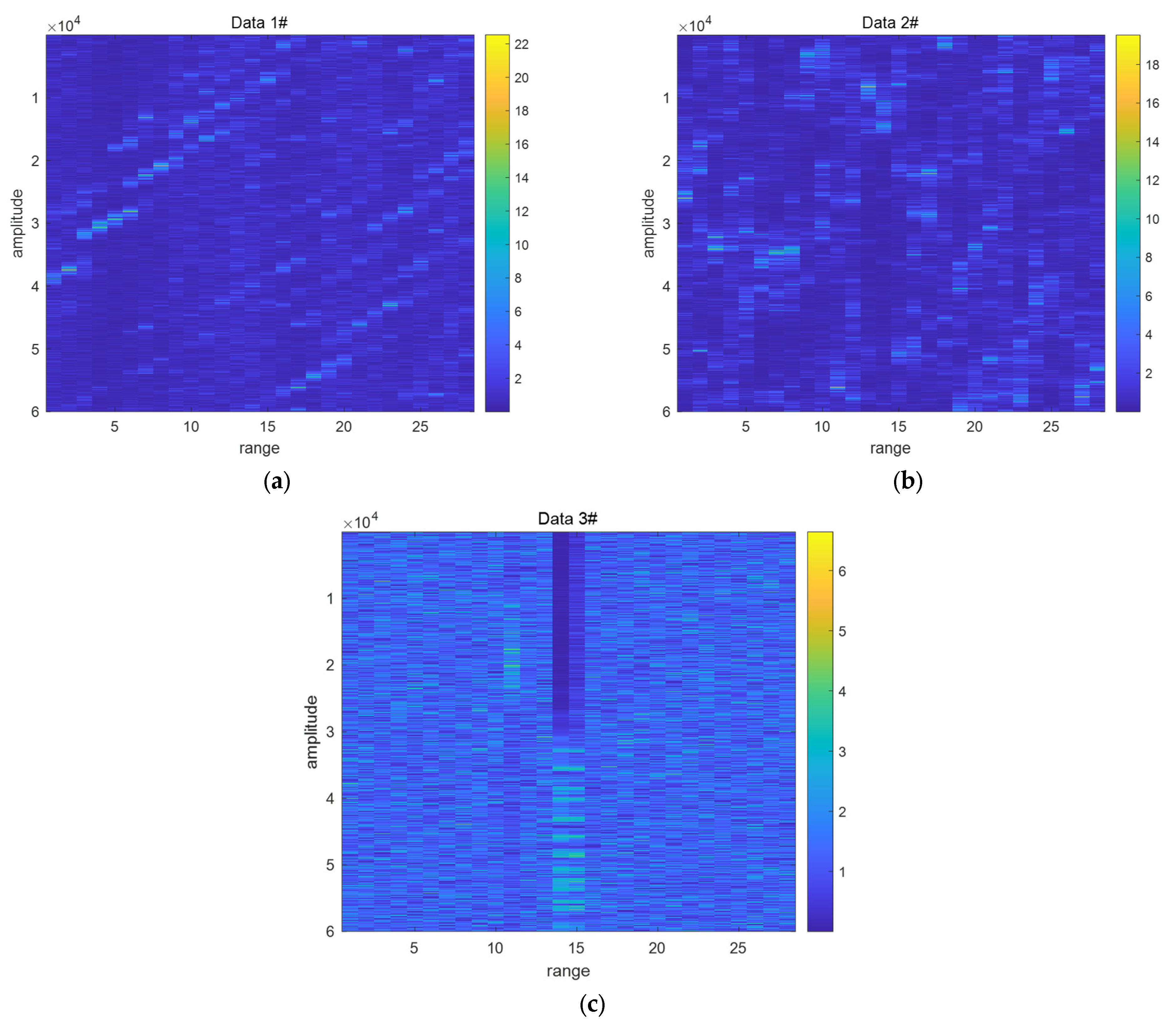
In this section, the real measured X-band sea clutter data are taken to analyze the performance of the proposed parameter estimation method. The real X-band sea clutter dataset is collected with McMaster University IPIX radar in 1998, the IPIX radar operates in gaze mode. The main parameter of IPIX radar is shown in

Table 1. Main radar parameters.

Parameter Type	Data 1#	Data 2#	Data 3#
Radar height	30 m	30 m	30 m
Band width	5 MHz	5 MHz	5 MHz
Range resolution	30 m	30 m	30 m
Beam width	0.9°	0.9°	0.9°
PRF	1000 Hz	1000 Hz	1000 Hz
Frequency	9.3 GHz	9.3 GHz	9.3 GHz
Operation mode	Grazing	Grazing	Grazing
Sea state	4	3	2

and the range–time-intensity image of the sea clutter datasets is shown in Figure 3, where Data 1# are under high sea state, Data 2# are under middle sea state and Data 3# are under low sea state. From Figure 3, it can be confirmed that the number and amplitude intensity of sea spikes are larger under a high sea state.

3.2. Parameter Estimation Analysis of Statistical Model

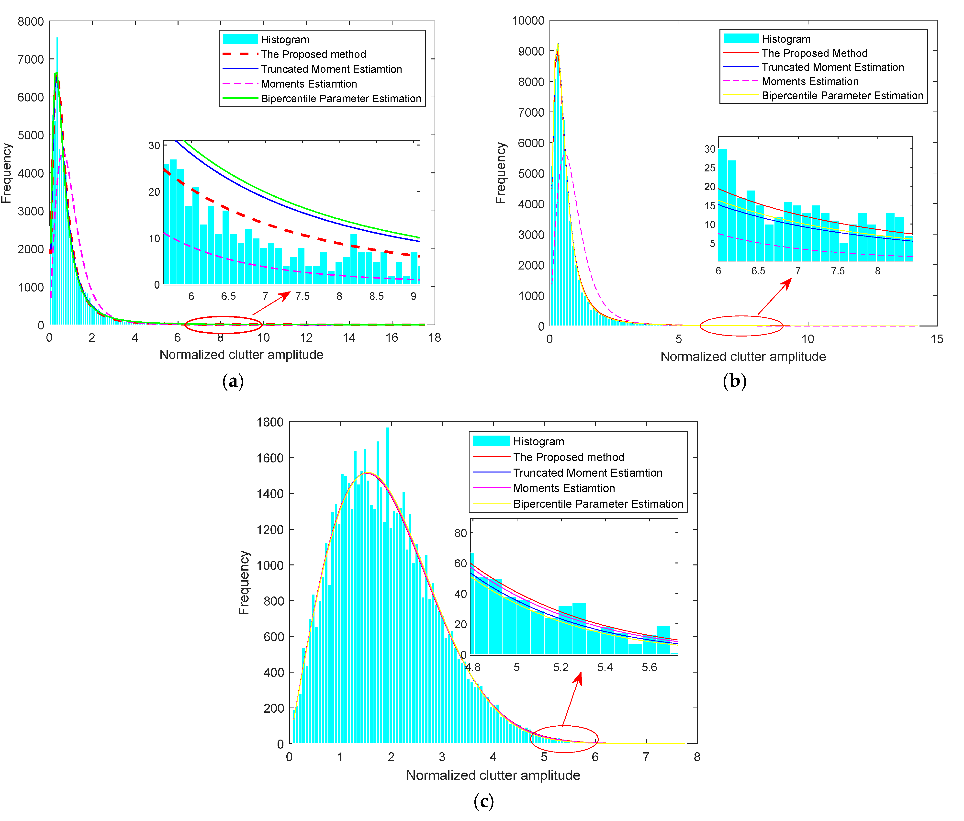
In this section, real measured sea clutter datasets of different range bins are selected to analyze the parameter estimation performance of the GP distribution. Then, the GP distribution parameters are estimated by the proposed method according to the calculation procedures in Section 2. For contrast, the BiP and truncated moment estimation methods are also analyzed. Figure 4a shows the histograms and theoretical distribution curves of the overall amplitude PDF based on different parameter estimation methods under a high sea state. Except for the purple dotted curve estimated by the traditional second-fourth MoM method, the other curves can match the sea clutter datasets well in Figure 4a. Likewise, it was also found that the fitted curve of MoM deviates far from the statistical histogram in Figure 4b, which indicates that the emergency of sea spikes with an increasing sea state will severely influence the performance of the MoM estimator. The histogram of data #3 and the PDF of fitted curves based on the four parameter estimation methods are shown in Figure 4c. From Figure 4c, it was found that the red curve fitted by the proposed method has a better matching effect with the statistical histogram, especially in the tail part. The more detailed discussion of the distribution model-matched results are analyzed from the GOF methods in the next section.

3.3. Analysis of the GOF Results

In this section, the GOF results of the GP distribution are tested by the MSD, K-S and MMSD methods. Since the matching effect of the curve fitted by the MoM is inferior under a higher sea state and when the variable interval takes almost the entire sea clutter sequence to perform parameter estimation under a lower sea state, the proposed method will degenerate MoM. Therefore, the MSD, MMSD and K-S distance are calculated respectively based on BiP, truncated moment estimation and the proposed method.

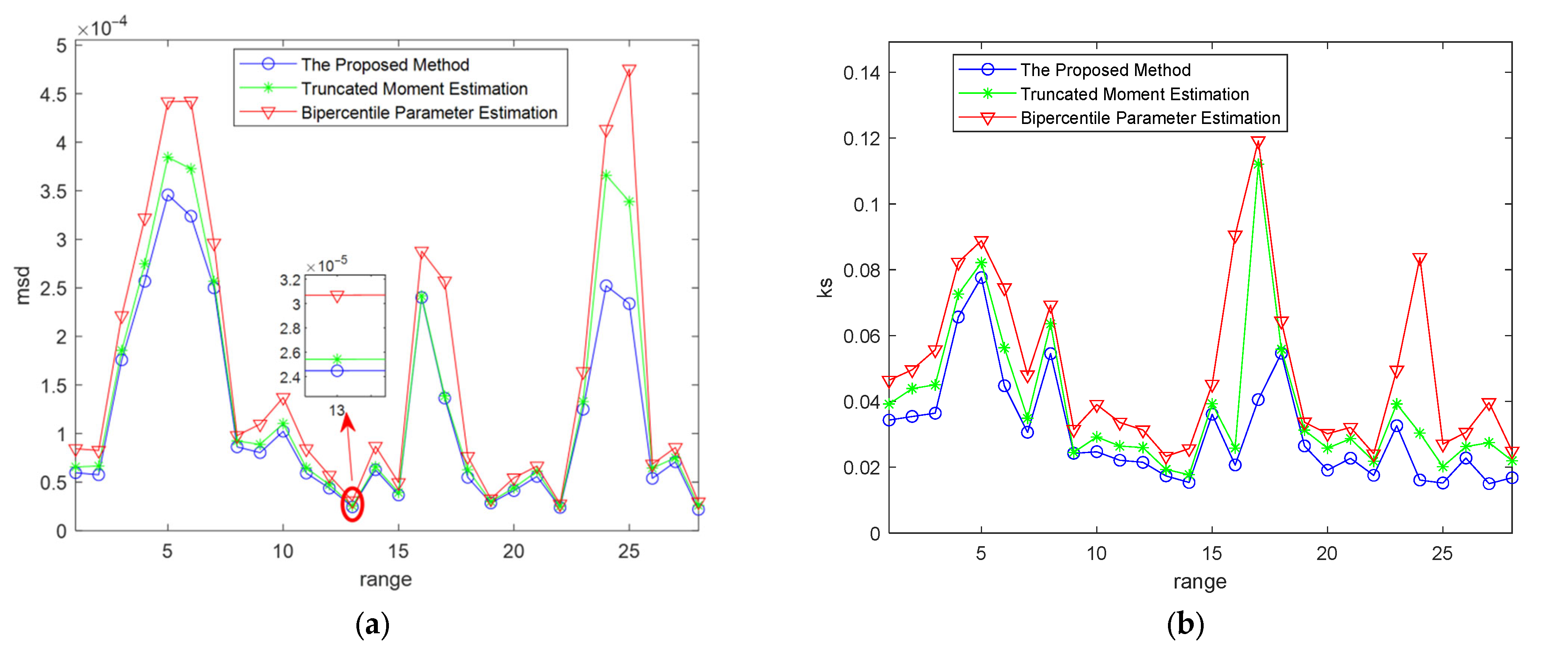
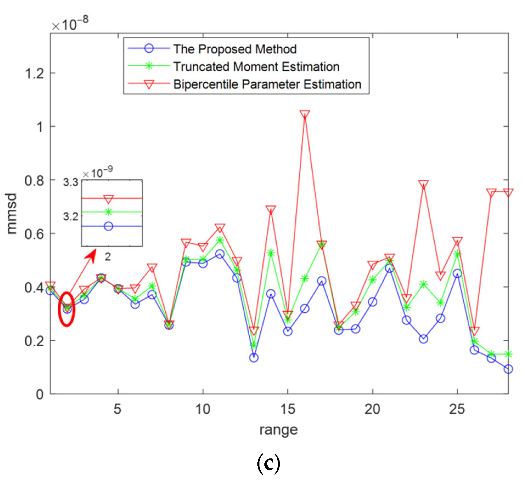
Figure 5, Figure 6 and Figure 7 show the GOF results of three parameter estimation methods in different range bins under different sea states. Since the sea state of Data 1# in Figure 5 is about 4, the interval is selected in the middle and tail part of the sea clutter series according to criterion discussed in Section 2. From Figure 5, it was found that the MSD and K-S results based on BiP and the truncated are worse because the BiP method only uses a pair of amplitude values in sea clutter series, which affects the accuracy and stability of parameter estimation, and the truncated method is unable to adjust the initial position of the sea clutter sequence for parameter estimation according to the statistical feature of the sea clutter, while the proposed method has the smallest MSD and K-S results, which represents the effectiveness of the proposed method. This is because the proposed method not only takes advantage of the information of bipercentile points, but it also utilizes the partial properties of the sea clutter series, which can better adjust the interval location according to the statistical feature of the sea clutter. Moreover, it can also be found that the MMSD results based on the proposed method are the smallest, which mean that the proposed VIE method can also improve the parameter estimation performance of the tail part of the PDF, which is helpful to perform target detection and to decrease the false alarm rate.

Moreover, the experiment based on Data 2# is also analyzed. Since the sea state of Data 2# is collected under a middle sea state, the interval is selected in the middle part of the sea clutter series. Figure 6 shows the GOF results of Data 2#. From Figure 6, it was found that the parameter estimation performance of the proposed method is better than that of the other methods, which is consistent with the results in Figure 5.

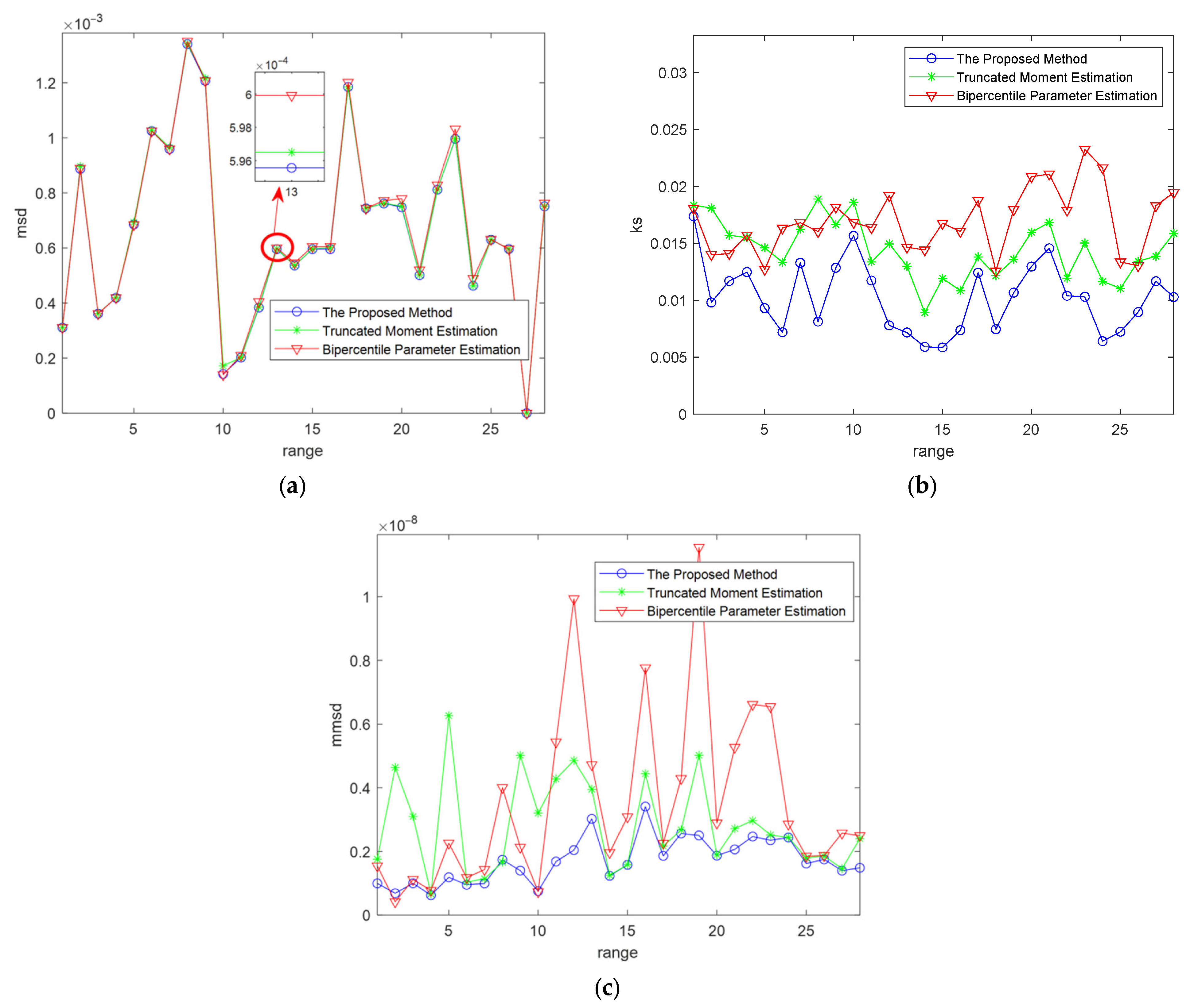
To further analyze the model-matching effect of the three parameter estimation methods, we have also performed the GOF experiment based on Data 3#. Since the sea state of Data 3# is relatively low, the interval is selected in the front and middle part of sea clutter sequences. From Figure 7a, it was found that the MSD results of the three parameter estimations are similar when the sea state is relatively low. The reason is that the number of sea spikes in the sea clutter sequences decreases, and the distribution of the sea clutter amplitude statistical histogram becomes more homogeneous under a low sea state condition. Nevertheless, the proposed method is still able to improve the accuracy of parameter estimation from the MSD, K-S and MMSD results in Figure 6.

To summarize, from the real sea clutter results analyzed in Figure 5, Figure 6 and Figure 7, we can conclude that the proposed VIE method has a better parameter estimation performance than the other method under either sea state. Moreover, we can find that the parameter estimation performance of the proposed method gradually increases with the increase in the sea state level. This phenomenon indicates that the proposed method has a better performance improvement for parameter estimation under a higher sea state, which contributes to a decrease in the false alarm rate and enhances target detection performance under complex sea clutter background.

To further illustrate the effectiveness of the proposed method, the other 200 range bins are randomly selected from 10 IPIX datasets to perform parameter estimation, and the mean values of the MSD, MMSD and K-S results from the 200 different sea clutter range bins are calculated, and the results are shown in

Table 2. Different parameter estimation performance analyses.

Parameter Estimation Method	MSD	K-S	MMSD
Proposed method	$\mathrm{}5.865\times {10}^{-4}$	$4.09\times {10}^{-2}$	$1.0332\times {10}^{-9}$
BIP method [31]	$9.673\times {10}^{-4}$	$5.395\times {10}^{-2}$	$1.968\times {10}^{-9}$
truncated moment estimation method [32]	$6.091\times {10}^{-4}$	$4.595\times {10}^{-2}$	$2.655\times {10}^{-9}$

. From Table 2, it was found that the results of MSD, K-S and MMSD based on the proposed method is smallest, which proves the effectiveness of the proposed method.

3.4. Parameter Performance Analysis through Monte Carlo Experiments

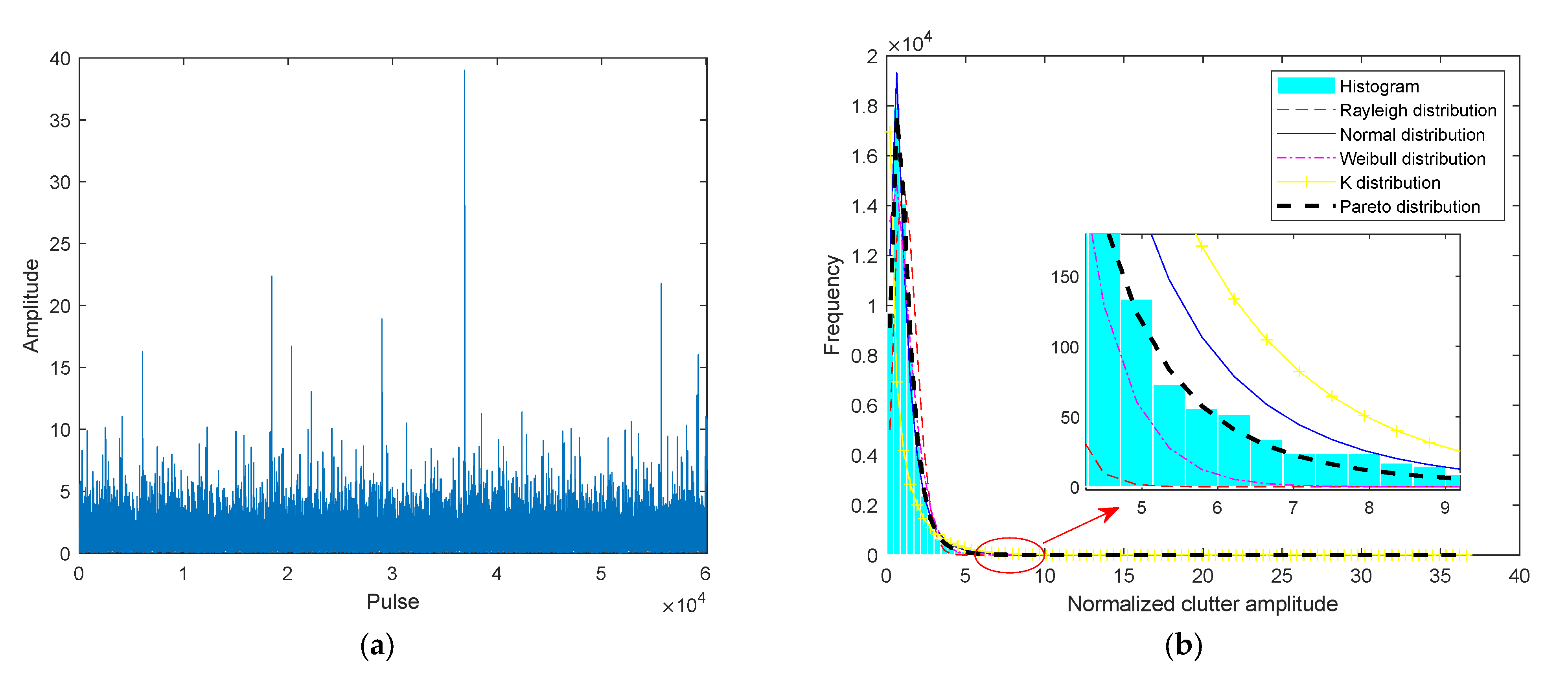
In Section 3.3, the GOF results of the parameter estimation method was analyzed through real sea clutter datasets. To further analyze the performance of the proposed VIE method, we performed the Monte Carlo experiments to enhance the persuasiveness of the proposed method. In this section, the spherically invariant random process (SIRP) method is taken to generate the simulated sea clutter data, which obey GP distribution with different parameters [33,34,35,36,37,38,39,40]. The simulated sea clutter amplitude series are shown in Figure 8a. While the histogram of simulated sea clutter series and the theoretical distribution curves are shown in Figure 8b. In Figure 8a, to make the generated sea clutter data closer to the real data, the larger-amplitude echoes have been added to simulate the sea spikes. From the results in Figure 8b, it was found that Rayleigh distribution, Log-normal distribution, Weibull distribution and K distribution fit worse to the simulated sea clutter data, while the Pareto distribution matched the data well. The results above confirm the validity of the simulated sea clutter.

Through the simulated sea clutter datasets, we performed 1000 times independent replicated experiments to estimate the parameters of GP distribution based on the four mentioned methods discussed in the paper. Then, the relative mean square error (RMSE) of the shape parameter $\lambda$ and scale parameter $a$ were calculated, and the formula for calculating the RMSE of shape parameter $\lambda$ is shown as follows:

$$RMS{E}_{\lambda }=\frac{1}{L}{{\displaystyle \sum _{i=1}^L\left(\frac{{\widehat{\lambda }}_i-\lambda }{\lambda }\right)}}^2$$

(29)

where $L$ represents the times of independent replicate experiment, ${\widehat{\lambda }}_i$ represents the estimated value of the shape parameter $\lambda$, and the RMSE of the scale parameter $a$ is also calculated as follows:

$$RMS{E}_a=\frac{1}{L}{{\displaystyle \sum _{i=1}^L\left(\frac{{\widehat{a}}_i-a}{a}\right)}}^2$$

(30)

where ${\widehat{a}}_i$ represents the estimated value of scale parameter $a$, and $L$ represents the times of the independent replicate experiment.

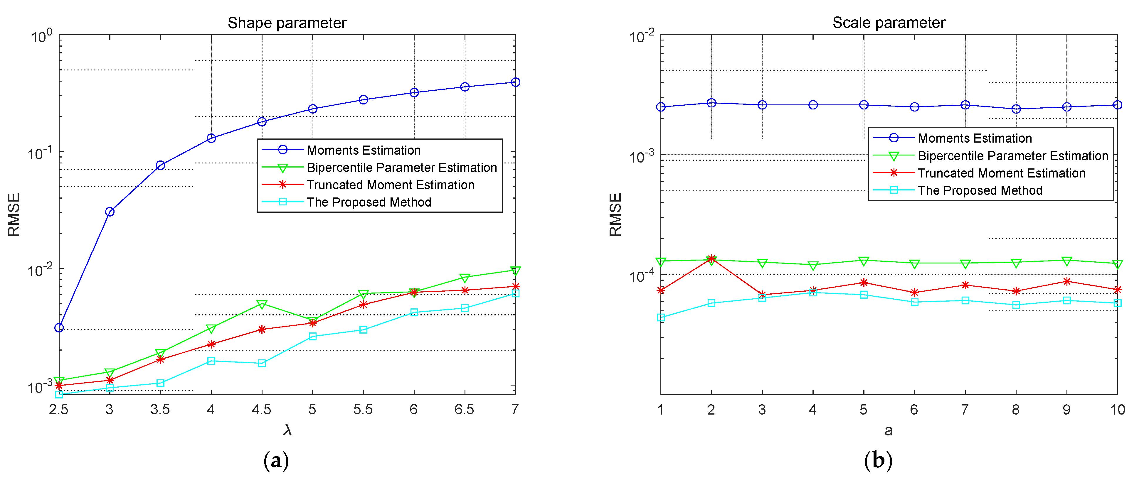
The calculation results of the RMSE are shown in Figure 9a, which represent the RMSE calculation results of shape parameter $\lambda$ , and Figure 9b represents the RMSE calculation results of scale parameter $a$. From Figure 9, the cyan curve represents the calculation results of RMSE based on the proposed method, both the shape parameter and scale parameter have smaller RMSE calculation results than that of the other three methods. Therefore, we can conclude that the proposed method has a higher parameter estimation accuracy, which indicates that the proposed parameter estimation method has better performance.

4. Conclusions

This paper mainly emphasized the parameter estimation of the GP distribution model of sea clutter. To overcome the shortcomings of the MoM-based parameter estimation methods, a novel parameter estimation method based on variable intervals was proposed for GP distribution. Considering the local properties of sea clutter, we took a variable interval of the entire sea clutter series for parameter estimation, where the interval position was selected according to the sea state conditions. Moreover, the zero-moment was constructed as a part of the proposed parameter estimator, which could increase the parameter estimation accuracy. Through the analysis of real measured sea clutter data, the proposed method had a better parameter estimation performance than the state-of-the-art moments estimators. The proposed algorithm was applicable for small radar observation scenarios, which belong to the same sea state. For large radar observation conditions with different sea states, the proposed method should be combined with the sea state separation method. For future practical system applications, the sea state should be a priori obtained or estimated before using the VIE method

References

1. Ward, K.; Tough, R.; Watts, S. Sea Clutter: Scattering, the K Distribution and Radar Performance, 2nd ed.; The Institution of Engineering and Technology: London, UK, 2013. [Google Scholar]
2. Ward, K.D.; Tough, R.J.A.; Watts, S. Sea clutter: Scattering, the K distribution and radar performance. Waves Random Complex Media 2013, 17, 233–234. [Google Scholar] [CrossRef]
3. Ravid, R.; Levanon, N. Maximum-likelihood CFAR for Weibull background. Radar Signal Processing Iee Proc. F 1992, 139, 256–264. [Google Scholar] [CrossRef]
4. Weik, M.H. Rayleigh distribution. In Encyclopedia of Statistical Sciences; Elsevier Ltd.: Amsterdam, The Netherlands, 2000; p. 1416. [Google Scholar]
5. Xin, Z.; Liao, G.; Yang, Z.; Zhang, Y.; Dang, H. Analysis of Distribution Using Graphical Goodness of Fit for Airborne SAR Sea-Clutter Data. IEEE Trans. Geosci. Remote Sens. 2017, 55, 5719–5728. [Google Scholar] [CrossRef]
6. Fan, Y.; Tao, M.; Su, J.; Wang, L. Analysis of goodness-of-fit method based on local property of statistical model for airborne sea clutter data. Digit. Signal Process. 2020, 99, 102653. [Google Scholar] [CrossRef]
7. Zhang, J.; Liu, F.; Liu, Y.; Wu, H.; Wu, W.; Zhou, A. A Study of Accelerated Life Test of White OLED Based on Maximum Likelihood Estimation Using Lognormal Distribution. IEEE Trans. Electron Devices 2012, 59, 3401–3404. [Google Scholar] [CrossRef]
8. Levanon, N. Order statistic CFAR for Weibull background. IEE Proc. Part F 1990, 137, 157–162. [Google Scholar]
9. Sarhan, A.M.; Zaindin, M. Modified Weibull distribution. Appl. Sci. 2009, 55, 189–200. [Google Scholar]
10. Carretero-Moya, J.; Gismero-Menoyo, J.; Blanco-del-Campo, Á.; Asensio-Lopez, A. Statistical Analysis of a High-Resolution Sea-Clutter Database. IEEE Trans. Geosci. Remote Sens. 2010, 48, 2024–2037. [Google Scholar] [CrossRef]
11. Johnsen, T. Characterization of X-band radar sea-clutter in a limited fetch condition from low to high grazing angles. In Proceedings of the 2015 IEEE Radar Conference, Arlington, VA, USA, 10–15 May 2015; pp. 109–114. [Google Scholar]
12. Huang, P.; Zou, Z.; Xia, X.-G.; Liu, X.; Liao, G. A Statistical Model Based on Modified Generalized-K Distribution for Sea Clutter. IEEE Geosci. Remote Sens. Lett. 2021, 19, 8015805. [Google Scholar] [CrossRef]
13. Arnold, B. Pareto Distributions, 2nd ed.; Taylor & Francis: Abingdon, UK, 2015; pp. 41–47. [Google Scholar]
14. Farshchian, M.; Posner, F.L. The Pareto distribution for low grazing angle and high resolution X-band sea clutter. In Proceedings of the 2010 IEEE Radar Conference, Arlington, VA, USA, 10–14 May 2010. [Google Scholar]
15. Weinberg, G.V. An Investigation of the Pareto Distribution as a Model for High Grazing Angle Clutter; Defence Science and Technology Organisation: Canberra, Australia, 2011. [Google Scholar]
16. Rosenberg, L.; Bocquet, S. The Pareto distribution for high grazing angle sea-clutter. In Proceedings of the IEEE Geoscience & Remote Sensing Symposium, Quebec City, QC, Canada, 13–18 July 2014; pp. 4209–4212. [Google Scholar]
17. Weinberg, G.V. Constant false alarm rate detectors for pareto clutter models. IET Radar Sonar Navig. 2013, 7, 153–163. [Google Scholar] [CrossRef]
18. Shang, X.; Song, H. Radar detection based on compound-Gaussian model with inverse gamma texture. IET Radar Sonar Navig. 2011, 5, 315–321. [Google Scholar] [CrossRef]
19. Stinco, P.; Greco, M.; Gini, F. Adaptive detection in compound-Gaussian clutter with inverse-gamma texture. In Proceedings of the 2011 IEEE CIE International Conference on Radar, Chengdu, China, 24–27 October 2011. [Google Scholar]
20. Chen, S.; Kong, L.; Yang, J. Adaptive Detection in Compound-Gaussian Clutter with Inverse Gaussian Texture. Cancer Res. 2013, 54, 2462–2467. [Google Scholar] [CrossRef] [Green Version]
21. Sangston, K.J.; Gini, F.; Greco, M.S. Coherent Radar Target Detection in Heavy-Tailed Compound-Gaussian Clutter. IEEE Trans. Aerosp. Electron. Syst. 2012, 48, 64–77. [Google Scholar] [CrossRef]
22. Weinberg, G.V. Coherent multilook detection for targets in Pareto distributed clutter. Electron. Lett. 2012, 47, 822–824. [Google Scholar] [CrossRef]
23. Banks, H.T.; Kunisch, K. Parameter Estimation: Basic Concepts and Examples; Birkhäuser Boston: Cambridge, MA, USA, 1989; pp. 53–91. [Google Scholar]
24. Balleri, A.; Nehorai, A.; Wang, J. Maximum likelihood estimation for compound-gaussian clutter with inverse gamma texture. IEEE Trans. Aerosp. Electron. Syst. 2007, 43, 775–779. [Google Scholar] [CrossRef]
25. Xu, S.; Wang, L.; Shui, P.; Li, X.; Zhang, J. Iterative maximum likelihood and zFlogz estimation of parameters of compound-Gaussian clutter with inverse gamma texture. In Proceedings of the 2018 IEEE International Conference on Signal Processing, Communications and Computing (ICSPCC), Qingdao, China, 14–16 September 2018; pp. 1–6. [Google Scholar]
26. Weinberg, G.V. Estimation of Pareto clutter parameters using order statistics and linear regression. Electron. Lett. 2013, 49, 845. [Google Scholar] [CrossRef]
27. Alexopoulos, A.; Weinberg, G.V. Fractional order Pareto distributions with application to X-band maritime radar clutter. Radar Sonar Navig. IET 2015, 9, 817–826. [Google Scholar] [CrossRef]
28. Mezache, A.; Chalabi, I.; Soltani, F.; Sahed, M. Estimating the Pareto plus noise distribution parameters using non-integer order moments and [zlog(z)] approaches. Radar Sonar Navig. IET 2016, 10, 192–204. [Google Scholar] [CrossRef] [Green Version]
29. Chan, D.; Rey, A.; Gambini, J.; Frery, A.C. Low-Cost Robust Estimation for the Single-Look Model Using the Pareto Distribution. IEEE Geosci. Remote Sens. Lett. 2020, 17, 1879-188. [Google Scholar] [CrossRef]
30. Mehanaoui, A.; Laroussi, T.; Mezache, A. New Pareto clutter parameters estimators based on log-moments and fractional negative-moments. In Proceedings of the 2017 Seminar on Detection Systems Architectures and Technologies (DAT), Algiers, Algeria, 20–22 February 2017; pp. 1–5. [Google Scholar]
31. Shui, P.; Yu, H.; Shi, L.; Yang, C. Explicit Bipercentile Parameter Estimation of Compound-Gaussian Clutter with Inverse Gamma Distributed Texture. IET Radar Sonar Navig. 2018, 12, 202–208. [Google Scholar] [CrossRef]
32. Hao, J.C. Research on the Parameter Moment Estimation Method of Sea Clutter Amplitude Distribution Based on Compound Gaussian Model. Master’s Thesis, Xidian University, Xian, China, 2017. [Google Scholar]
33. Yang, C.; Wei, Y.; Yang, W. Simulation of compound k-distribution sea clutter. In Proceedings of the IEEE Radar, Cie International Conference, Beijing, China, 8–10 October 1996. [Google Scholar]
34. Yang, J.L.; Wan, J.W. New Method for the Simulation of Coherent K-distributed Clutter. In Proceedings of the CIE International Conference on Radar, Shanghai, China, 16–19 October 2006; pp. 1–4. [Google Scholar]
35. Jie, Z.; Dong, C.; Sun, D.K. Distribution Sea Clutter Modeling and Simulation Based on ZMNL. In Proceedings of the IEEE International Conference on Intelligent Computation Technology & Automation, Nanchang, China, 14–15 June 2015. [Google Scholar]
36. Angelliaume, S.; Rosenberg, L.; Ritchie, M. Modeling the Amplitude Distribution of Radar Sea Clutter. Remote Sens. 2019, 11, 319. [Google Scholar] [CrossRef] [Green Version]
37. Huang, D.; Zeng, D.Z.; Long, T. A new method for modeling and simulation of coherent correlated K-distributed clutter. In Proceedings of the IET International Radar Conference, Guilin, China, 20–22 April 2009. [Google Scholar]
38. Yanhui, H.; Feng, L.; Baobao, Z.; Shunjun, W. Simulation of Coherent Correlation K-distribution Sea Clutter Based on SIRP. In Proceedings of the 2006 CIE International Conference on Radar, Shanghai, China, 16–19 October 2006; pp. 1–4. [Google Scholar]
39. Bocquet, S. Simulation of correlated Pareto distributed sea clutter. In Proceedings of the 2013 International Conference on Radar, Adelaide, Australia, 9–12 September 2013; pp. 258–261. [Google Scholar]
40. Bocquet, S.; Rosenberg, L.; Watts, S. Simulation of coherent sea clutter with inverse gamma texture. In Proceedings of the 2014 International Radar Conference, Lille, France, 3–17 October 2014; pp. 1–6. [Google Scholar]
Figure 1. Interval position selection sketch map.
Remotesensing 14 02326 g001
Figure 2. Flow chart of the proposed parameter estimation method.
Remotesensing 14 02326 g002
Figure 3. Range–time-intensity image of X-band radar echoes: (a) high sea state; (b) middle sea state; (c) low sea state.
Remotesensing 14 02326 g003
Figure 4. Histogram of measured sea clutter data: (a) high sea state (Data 1#); (b) middle sea state (Data 2#); (c) low sea state.
Remotesensing 14 02326 g004
Figure 5. GOF results under a high sea state: (a) Msd_results (Data 1#); (b) Ks_result (Data 1#); (c) Mmsd_results (Data 1#).
Remotesensing 14 02326 g005aRemotesensing 14 02326 g005b
Figure 6. GOF results under a middle sea state: (a) Msd_results (Data 2#); (b) Ks_result (Data 2#); (c) Mmsd_results (Data 2#).
Remotesensing 14 02326 g006
Figure 7. GOF results under a low sea state: (a) Msd_results (Data 3#); (b) Ks_result (Data 3#); (c) Mmsd_results (Data 3#).
Remotesensing 14 02326 g007
Figure 8. The simulated sea clutter sequence: (a) sea clutter amplitude sequence; (b) histogram of simulated data.
Remotesensing 14 02326 g008
Figure 9. RMSE calculation results of two parameters: (a) RMSE of shape parameter; (b) RMSE of scale parameter.
Remotesensing 14 02326 g009