
Investigation of Time-Lapse Changes with DAS Borehole Data at the Brady Geothermal Field Using Deconvolution Interferometry


Abstract
:1. Introduction
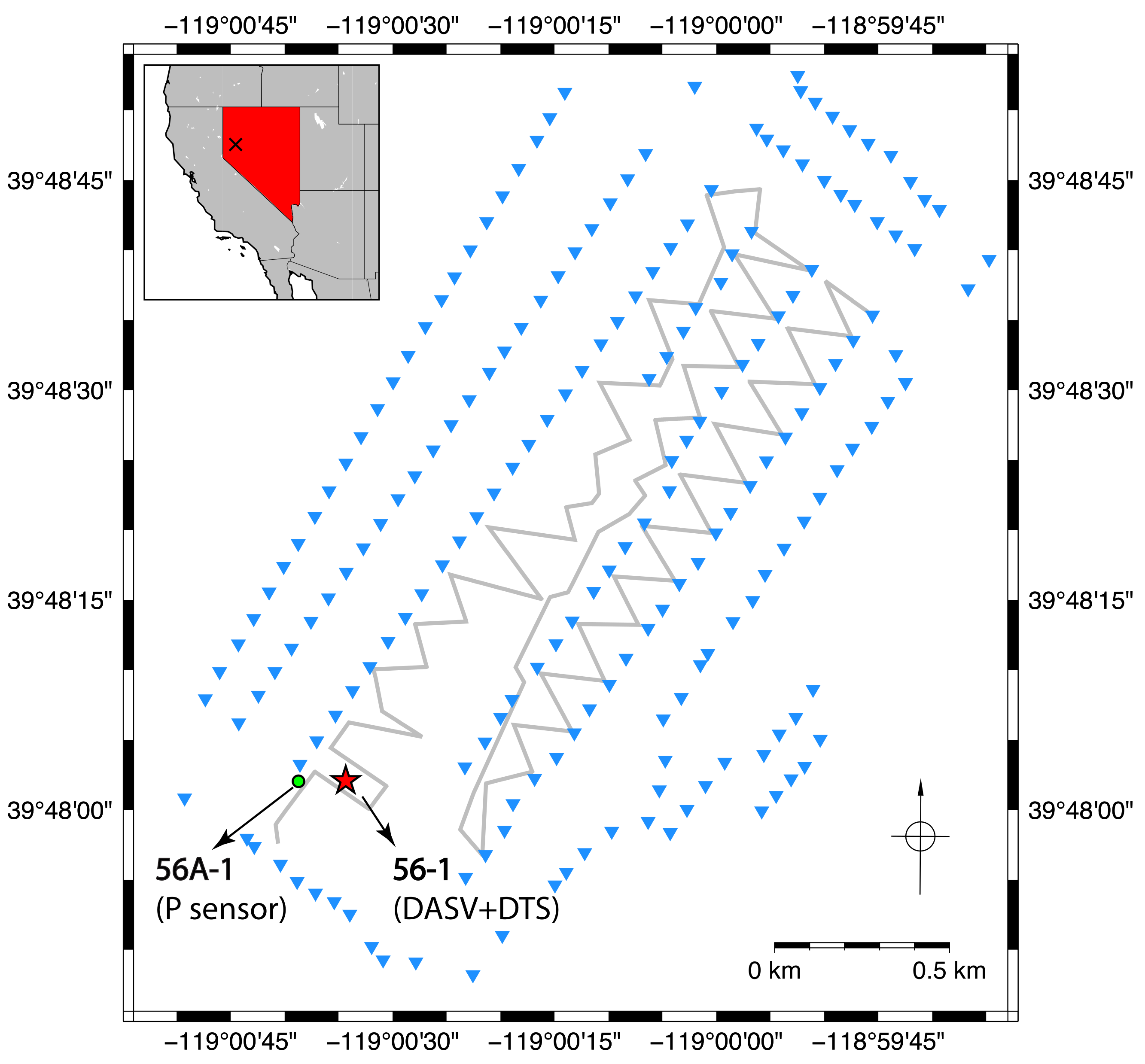
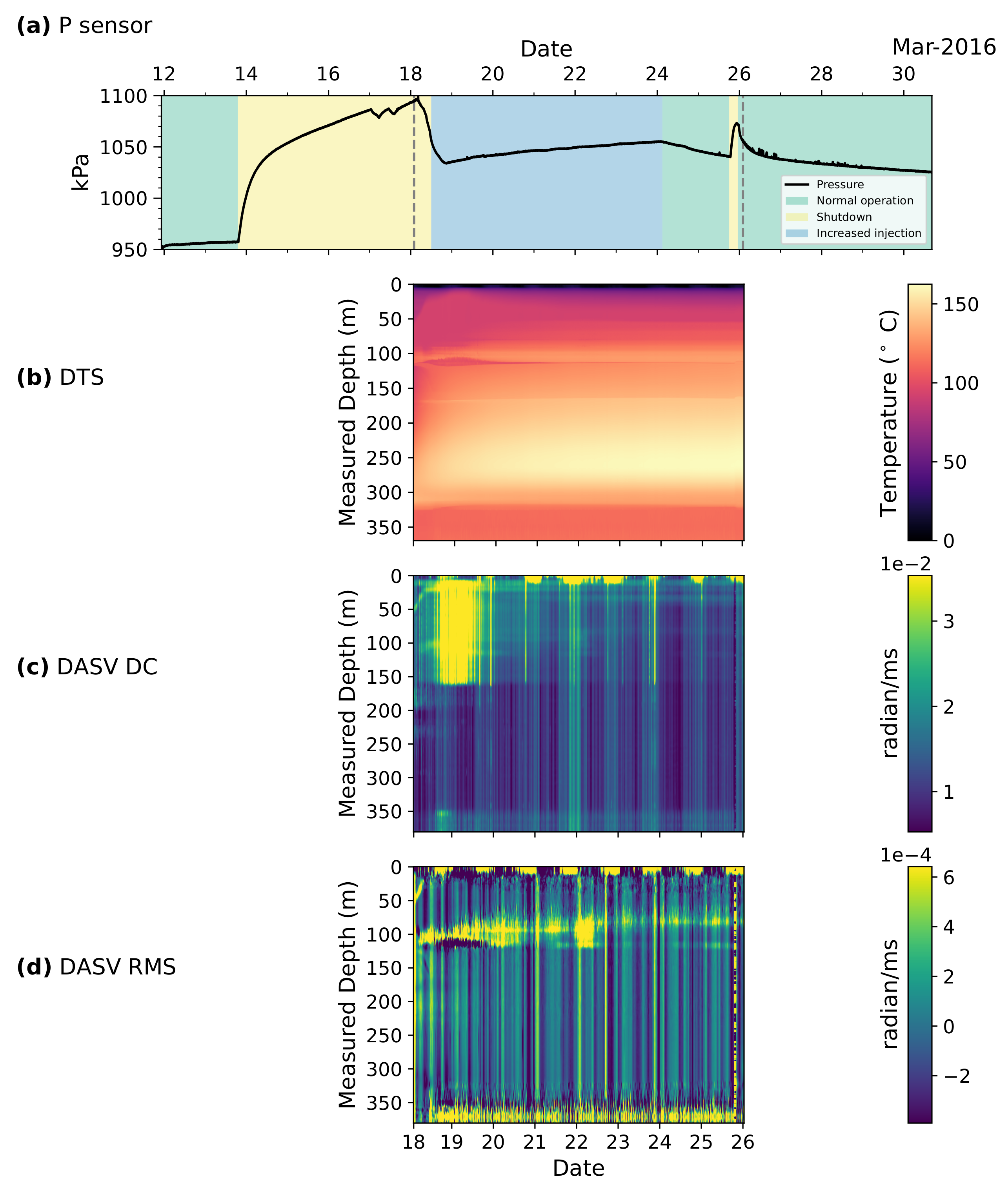
2. Data
3. Methods and Analysis
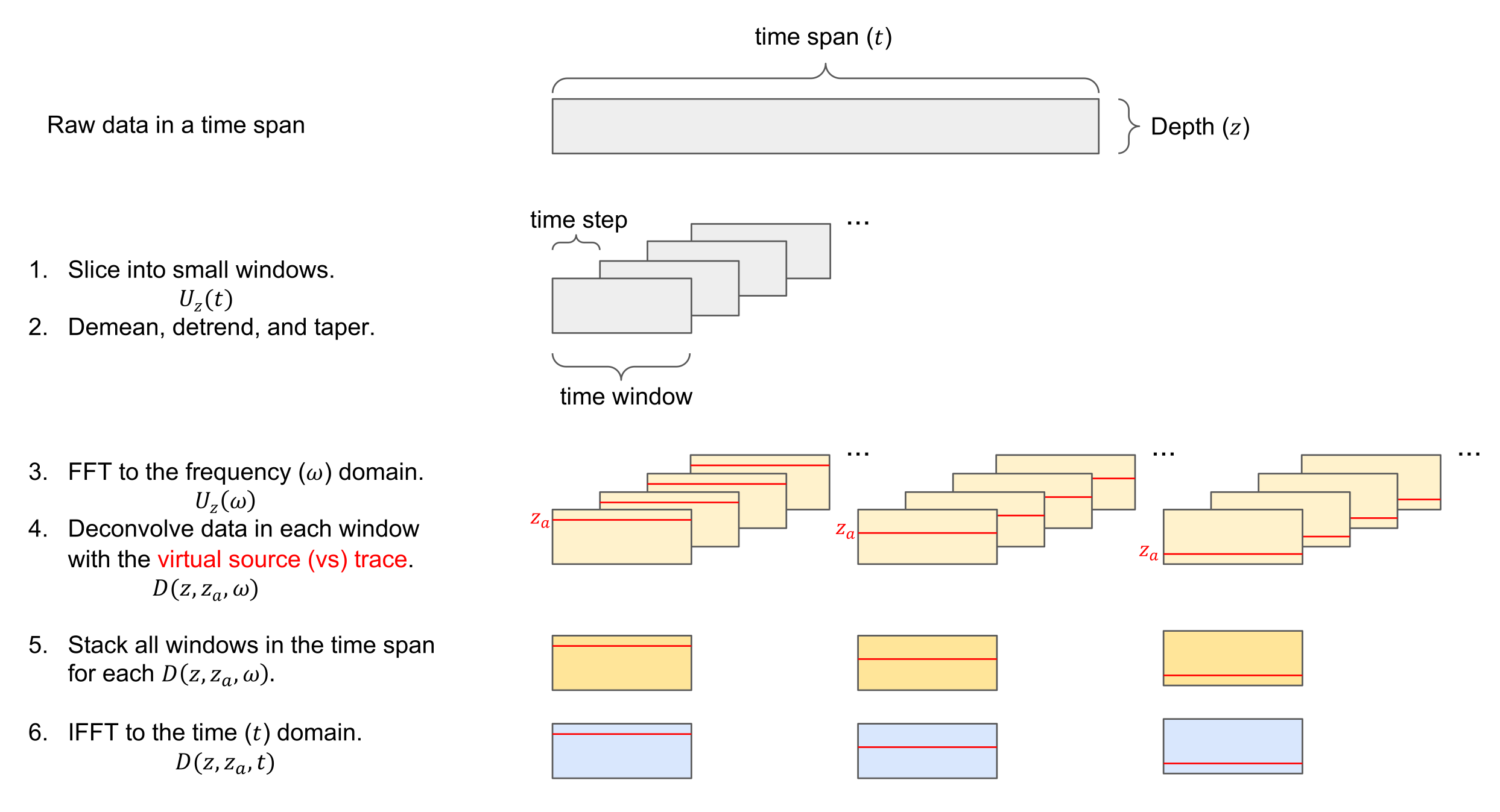
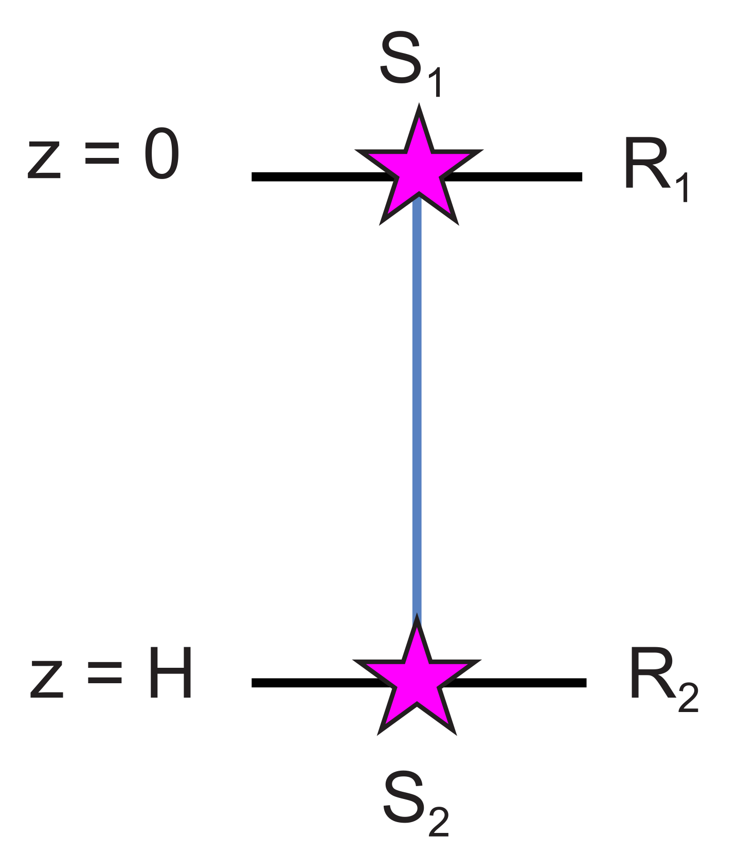
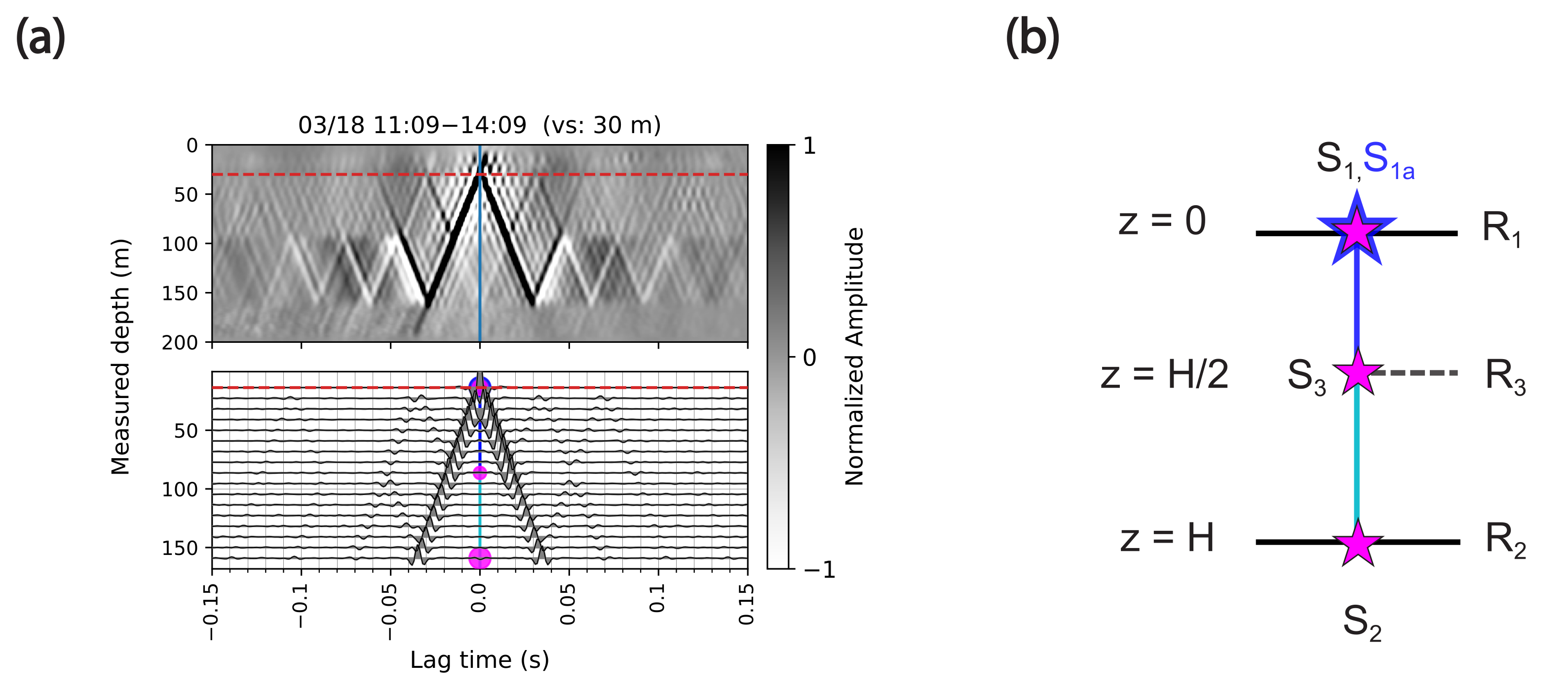
3.1. Review of Deconvolution Interferometry
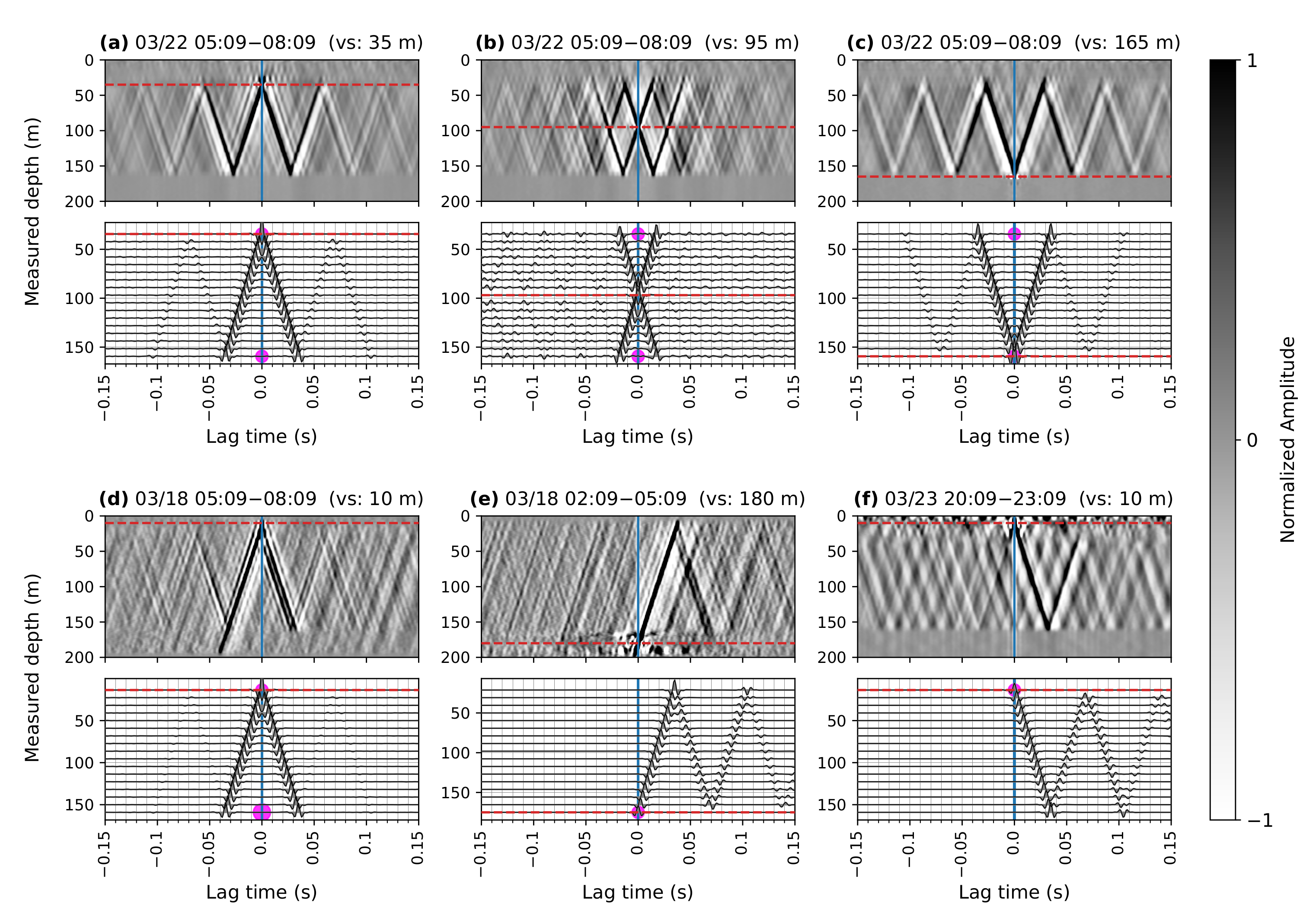
3.2. Deconvolved Wavefields
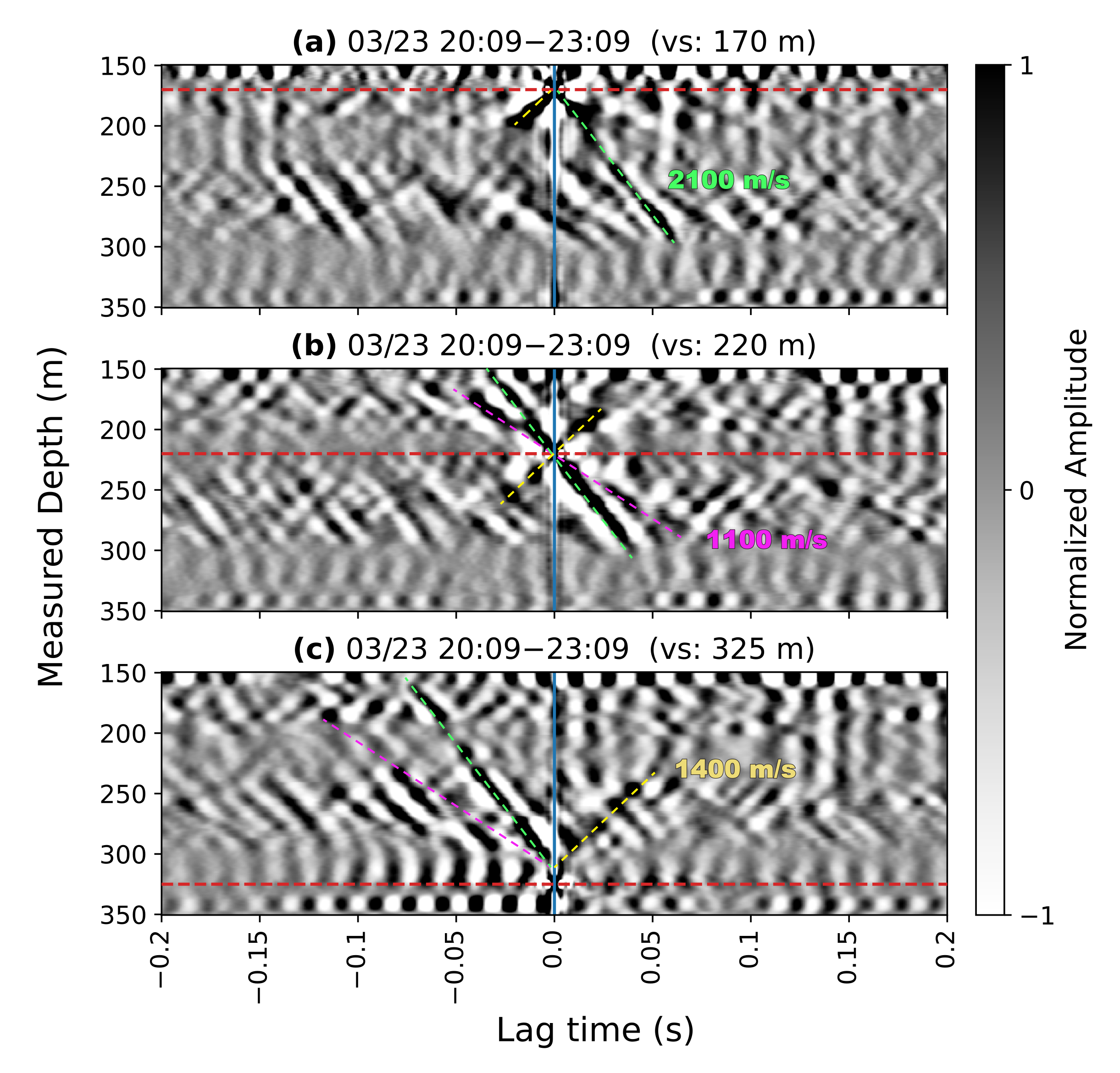
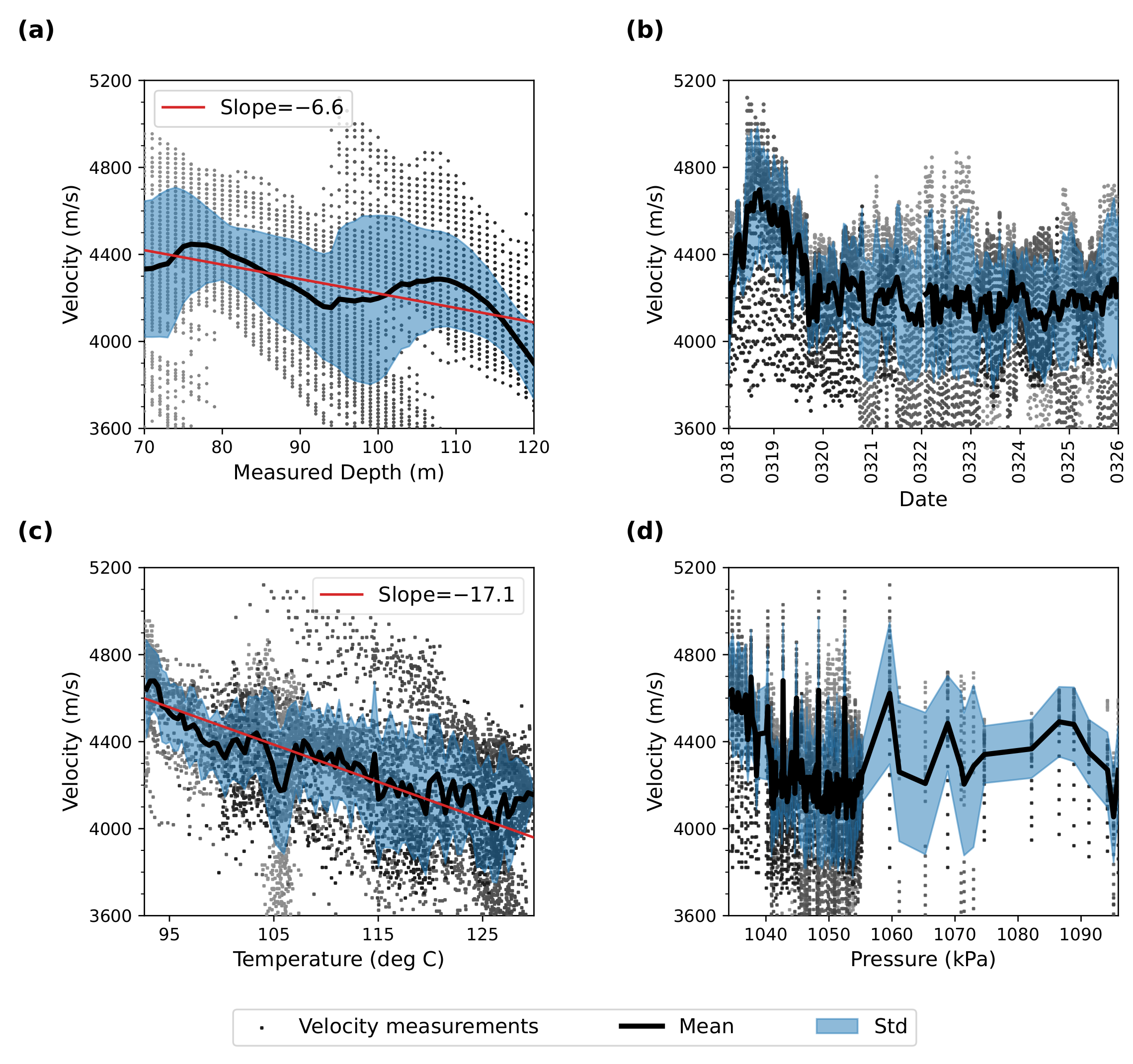
3.3. Time-Lapse Changes of Wave Velocities
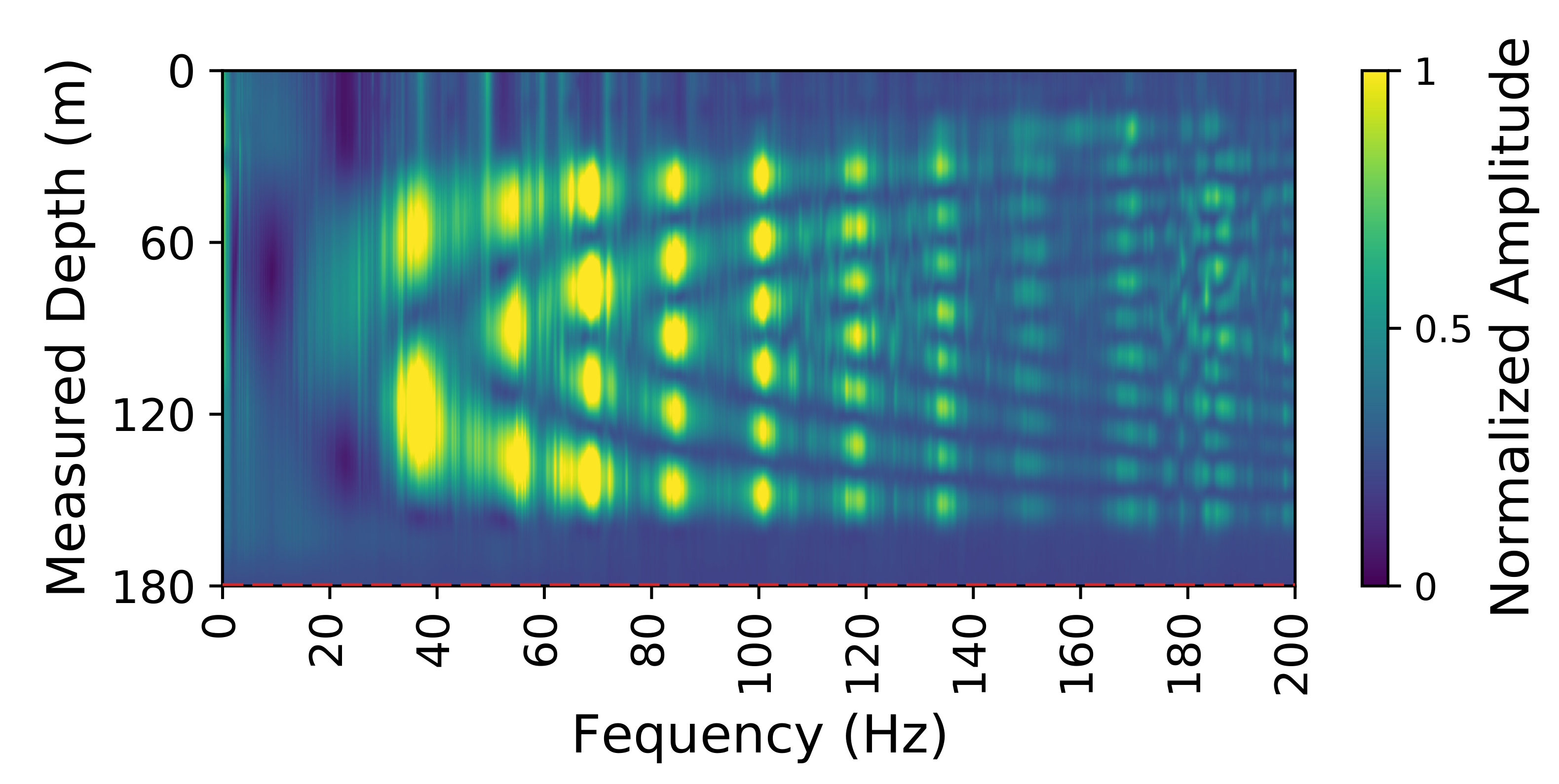
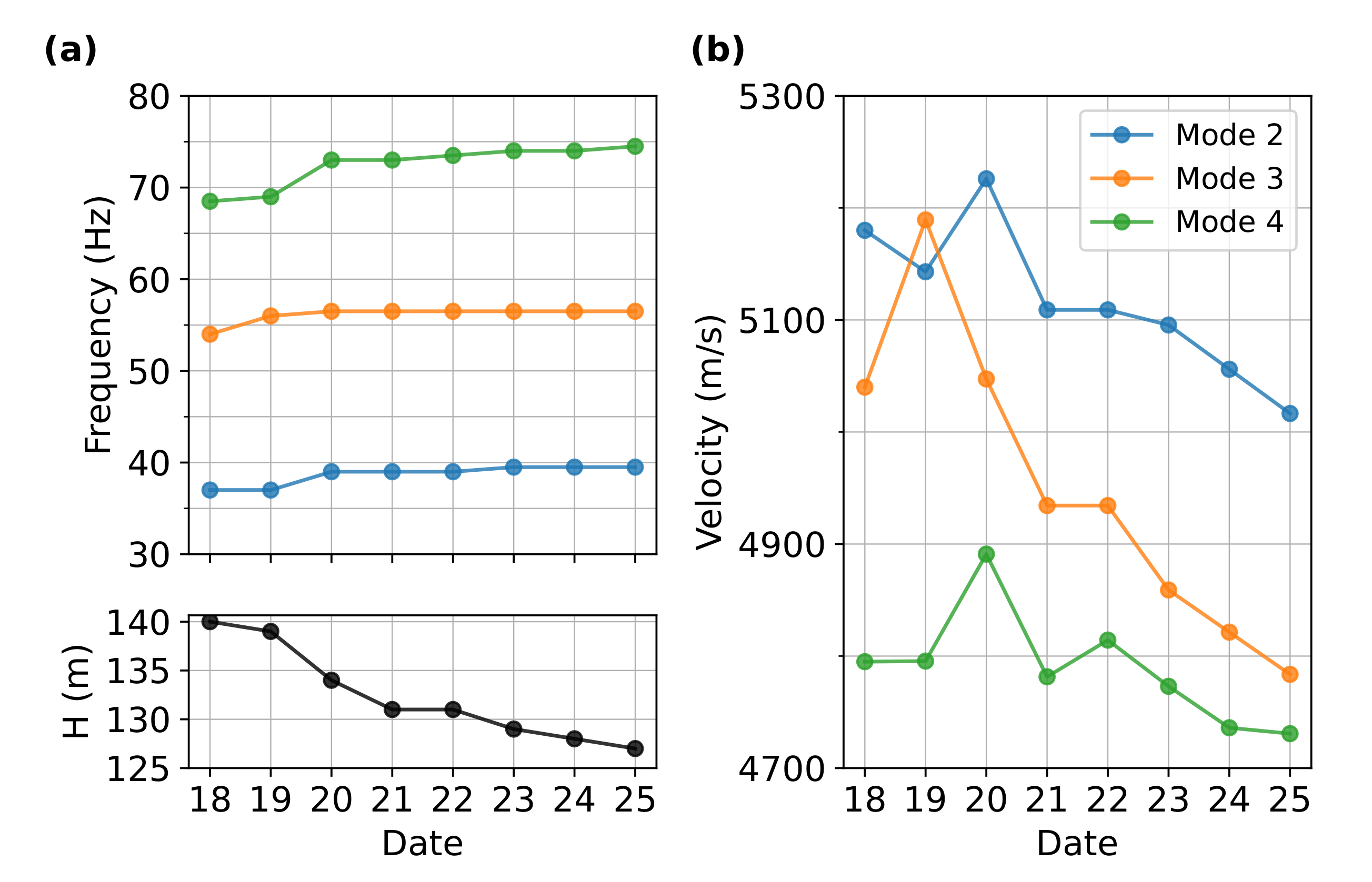
3.4. Normal-Mode Analysis
4. Discussions
5. Conclusions
Author Contributions
Funding
Institutional Review Board Statement
Informed Consent Statement
Data Availability Statement
Acknowledgments
Conflicts of Interest
Abbreviations
| DAS | Distributed acoustic sensing |
| DTS | Distributed temperature sensing |
| RMS | Root-mean-square |
Appendix A. Varying Model Parameters
Appendix A.1. The Effect of Source Correlation

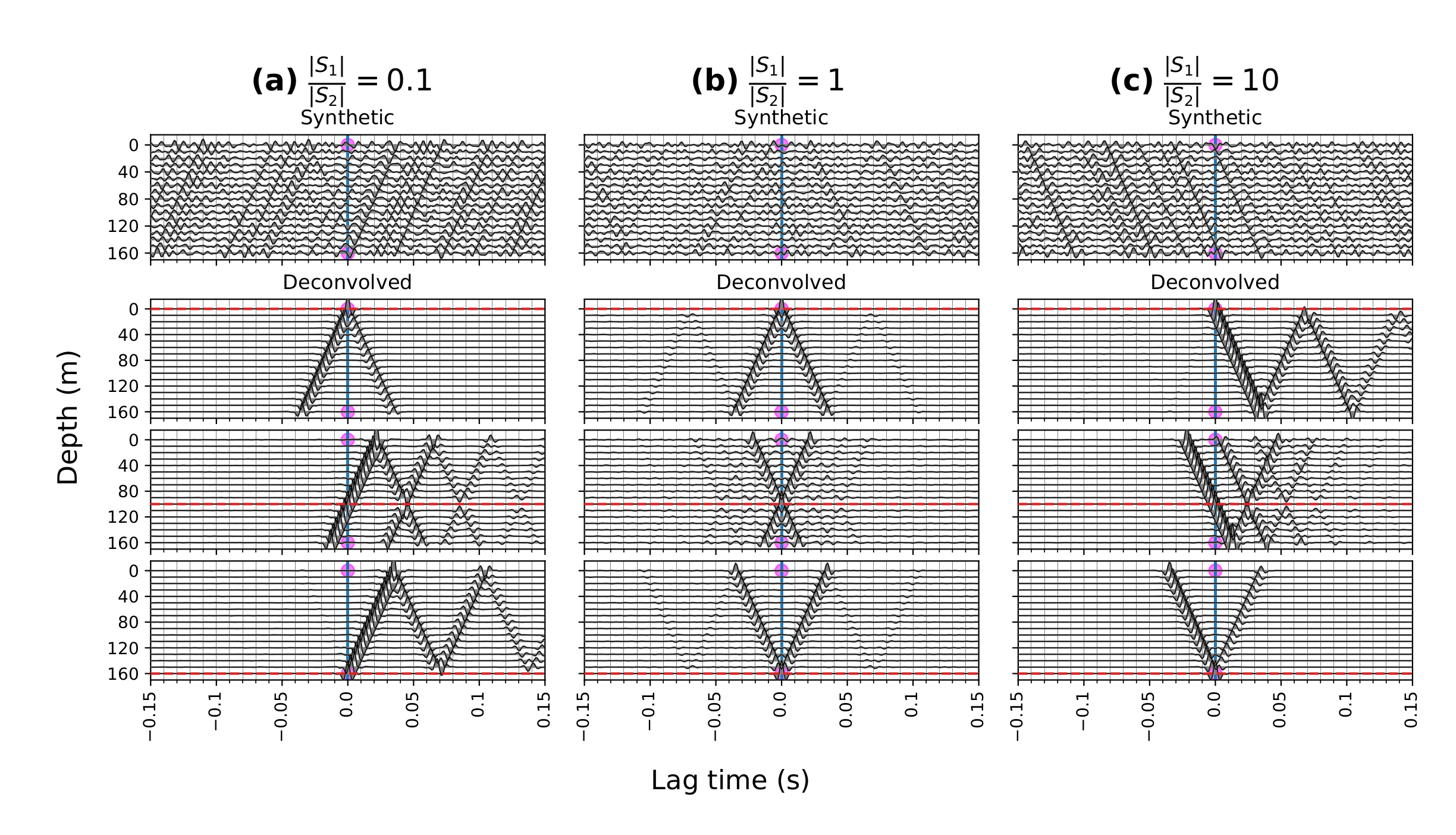
Appendix A.2. The Effect of Relative Source Amplitude
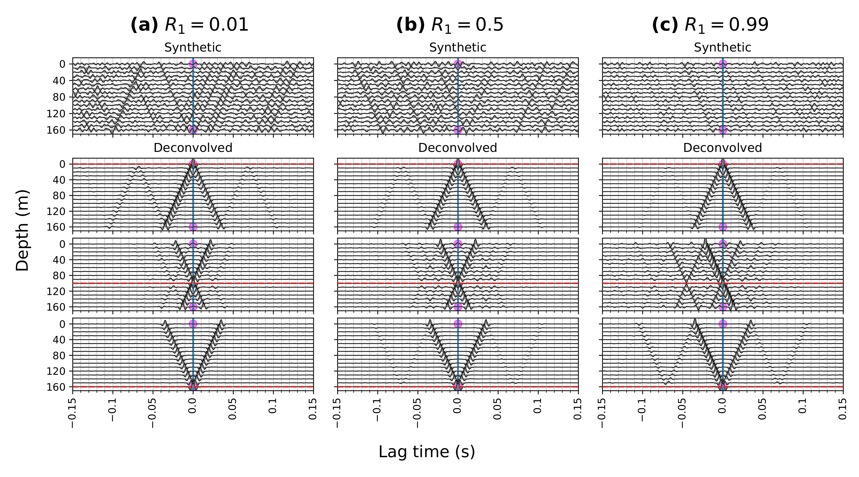
Appendix A.3. The Effect of Reflection Coefficients
Appendix B. Deconvolved Wavefields at the Lower Part below 200 M
References
- Baldwin, C.S. Brief history of fiber optic sensing in the oil field industry. In Fiber Optic Sensors and applications XI; International Society for Optics and Photonics: Bellingham, WA, USA, 2014; Volume 9098, p. 909803. [Google Scholar]
- Johannessen, K.; Drakeley, B.; Farhadiroushan, M. Distributed acoustic sensing—A new way of listening to your well/reservoir. In SPE Intelligent Energy International; OnePetro: Utrecht, The Netherlands, 27 March 2012. [Google Scholar]
- Finfer, D.C.; Mahue, V.; Shatalin, S.; Parker, T.; Farhadiroushan, M. Borehole flow monitoring using a non-intrusivepassive distributed acoustic sensing (DAS). In Proceedings of the SPE Annual Technical Conference and Exhibition, OnePetro, Amsterdam, The Netherlands, 27 October 2014. [Google Scholar]
- Naldrett, G.; Cerrahoglu, C.; Mahue, V. Production monitoring using next-generation distributed sensing systems. Petrophysics 2018, 59, 496–510. [Google Scholar] [CrossRef]
- Mateeva, A.; Lopez, J.; Potters, H.; Mestayer, J.; Cox, B.; Kiyashchenko, D.; Wills, P.; Grandi, S.; Hornman, K.; Kuvshinov, B.; et al. Distributed acoustic sensing for reservoir monitoring with vertical seismic profiling. Geophys. Prospect. 2014, 62, 679–692. [Google Scholar] [CrossRef]
- Daley, T.; Miller, D.; Dodds, K.; Cook, P.; Freifeld, B. Field testing of modular borehole monitoring with simultaneous distributed acoustic sensing and geophone vertical seismic profiles at Citronelle, Alabama. Geophys. Prospect. 2016, 64, 1318–1334. [Google Scholar] [CrossRef] [Green Version]
- Byerley, G.; Monk, D.; Aaron, P.; Yates, M. Time-lapse seismic monitoring of individual hydraulic-frac stages using a downhole DAS array. Lead. Edge 2018, 37, 802–810. [Google Scholar] [CrossRef]
- Correa, J.; Pevzner, R.; Bona, A.; Tertyshnikov, K.; Freifeld, B.; Robertson, M.; Daley, T. 3D vertical seismic profile acquired with distributed acoustic sensing on tubing installation: A case study from the CO2CRC Otway Project. Interpretation 2019, 7, SA11–SA19. [Google Scholar] [CrossRef]
- Jin, G.; Roy, B. Hydraulic-fracture geometry characterization using low-frequency DAS signal. Lead. Edge 2017, 36, 975–980. [Google Scholar] [CrossRef]
- Ghahfarokhi, P.K.; Wilson, T.H.; Carr, T.R.; Kumar, A.; Hammack, R.; Di, H. Integrating distributed acoustic sensing, borehole 3C geophone array, and surface seismic array data to identify long-period long-duration seismic events during stimulation of a Marcellus Shale gas reservoir. Interpretation 2019, 7, SA1–SA10. [Google Scholar] [CrossRef] [Green Version]
- Webster, P.; Wall, J.; Perkins, C.; Molenaar, M. Micro-seismic detection using distributed acoustic sensing. In SEG Technical Program Expanded Abstracts 2013; Society of Exploration Geophysicists: Tulsa, OK, USA, 2013; pp. 2459–2463. [Google Scholar]
- Hartog, A.H. An Introduction to Distributed Optical Fibre Sensors; CRC Press: Boca Raton, FL, USA, 2017. [Google Scholar]
- Bruno, M.S.; Lao, K.; Oliver, N.; Becker, M. Use of Fiber Optic Distributed Acoustic Sensing for Measuring Hydraulic Connectivity for Geothermal Applications; Technical report; GeoMechanics Technologies: Monrovia, CA, USA, 2018. [Google Scholar]
- Miller, D.E.; Coleman, T.; Zeng, X.; Patterson, J.R.; Reinisch, E.C.; Cardiff, M.A.; Wang, H.F.; Fratta, D.; Trainor-Guitton, W.; Thurber, C.H. DAS and DTS at Brady Hot Springs: Observations about coupling and coupled interpretations. In Proceedings of the 43rd Workshop on Geothermal Reservoir Engineering, Stanford, CA, USA, 12–14 February 2018; pp. 12–14. [Google Scholar]
- Miller, D.E.; Parker, T.R.; Kashikar, S.; Todorov, M.D.; Bostick, T. Vertical seismic profiling using a fibre-optic cable as a distributed acoustic sensor. In Proceedings of the 74th EAGE Conference and Exhibition incorporating SPE EUROPEC 2012, Copenhagen, Denmark, 4–7 June 2012. [Google Scholar]
- Barberan, C.; Allanic, C.; Avila, D.; Hy-Billiot, J.; Hartog, A.; Frignet, B.; Lees, G. Multi-offset seismic acquisition using optical fiber behind tubing. In Proceedings of the 74th EAGE Conference and Exhibition Incorporating EUROPEC 2012, Copenhagen, Denmark, 4–7 June 2012. [Google Scholar]
- Didraga, C. DAS VSP recorded simultaneously in cemented and tubing installed fiber optic cables. In Proceedings of the 77th EAGE Conference and Exhibition 2015, Madrid, Spain, 1–4 June 2015; European Association of Geoscientists & Engineers: Houten, The Netherlands, 2015; Volume 2015, pp. 1–5. [Google Scholar]
- Yu, G.; Cai, Z.; Chen, Y.; Wang, X.; Zhang, Q.; Li, Y.; Wang, Y.; Liu, C.; Zhao, B.; Greer, J. Walkaway VSP using multimode optical fibers in a hybrid wireline. Lead. Edge 2016, 35, 615–619. [Google Scholar] [CrossRef]
- Willis, M.E.; Wu, X.; Palacios, W.; Ellmauthaler, A. Understanding cable coupling artifacts in wireline-deployed DAS VSP data. In SEG Technical Program Expanded Abstracts 2019; Society of Exploration Geophysicists: Tulsa, OK, USA, 2013; pp. 5310–5314. [Google Scholar]
- Martuganova, E.; Stiller, M.; Bauer, K.; Henninges, J.; Krawczyk, C.M. Cable reverberations during wireline distributed acoustic sensing measurements: Their nature and methods for elimination. Geophys. Prospect. 2021, 69, 1034–1054. [Google Scholar] [CrossRef]
- Feigl, K.L.; Team, P. Overview and preliminary results from the PoroTomo project at Brady Hot Springs, Nevada: Poroelastic tomography by adjoint inverse modeling of data from seismology, geodesy, and hydrology. In Proceedings of the 42nd Workshop on Geothermal Reservoir Engineering, Stanford, CA, USA, 13–15 February 2017; pp. 1–15. [Google Scholar]
- Feigl, K.L.; Parker, L.M. PoroTomo Final Technical Report: Poroelastic Tomography by Adjoint Inverse Modeling of Data from Seismology, Geodesy, and Hydrology; Technical Report; University of Wisconsin: Madison, WI, USA, 2019. [Google Scholar]
- Patterson, J.R.; Cardiff, M.; Coleman, T.; Wang, H.; Feigl, K.L.; Akerley, J.; Spielman, P. Geothermal reservoir characterization using distributed temperature sensing at Brady Geothermal Field, Nevada. Lead. Edge 2017, 36, 1024a1–1024a7. [Google Scholar] [CrossRef] [Green Version]
- Patterson, J.R. Understanding Constraints on Geothermal Sustainability through Reservoir Characterization at Brady Geothermal Field, Nevada. Ph.D. Thesis, University of Wisconsin, Madison, WI, USA, 2018. [Google Scholar]
- Trainor-Guitton, W.; Guitton, A.; Jreij, S.; Powers, H.; Sullivan, B. 3D Imaging of Geothermal Faults from a Vertical DAS Fiber at Brady Hot Spring, NV USA. Energies 2019, 12, 1401. [Google Scholar] [CrossRef] [Green Version]
- Snieder, R.; Sheiman, J.; Calvert, R. Equivalence of the virtual-source method and wave-field deconvolution in seismic interferometry. Phys. Rev. E 2006, 73, 066620. [Google Scholar] [CrossRef] [Green Version]
- Snieder, R.; Miyazawa, M.; Slob, E.; Vasconcelos, I.; Wapenaar, K. A comparison of strategies for seismic interferometry. Surv. Geophys. 2009, 30, 503–523. [Google Scholar] [CrossRef]
- Nakata, N.; Snieder, R.; Kuroda, S.; Ito, S.; Aizawa, T.; Kunimi, T. Monitoring a building using deconvolution interferometry. I: Earthquake-data analysis. Bull. Seismol. Soc. Am. 2013, 103, 1662–1678. [Google Scholar] [CrossRef]
- Snieder, R.; Safak, E. Extracting the building response using seismic interferometry: Theory and application to the Millikan Library in Pasadena, California. Bull. Seismol. Soc. Am. 2006, 96, 586–598. [Google Scholar] [CrossRef] [Green Version]
- Nakata, N.; Snieder, R. Monitoring a building using deconvolution interferometry. II: Ambient-vibration analysis. Bull. Seismol. Soc. Am. 2014, 104, 204–213. [Google Scholar] [CrossRef]
- Sawazaki, K.; Sato, H.; Nakahara, H.; Nishimura, T. Time-lapse changes of seismic velocity in the shallow ground caused by strong ground motion shock of the 2000 Western-Tottori earthquake, Japan, as revealed from coda deconvolution analysis. Bull. Seismol. Soc. Am. 2009, 99, 352–366. [Google Scholar] [CrossRef]
- Yamada, M.; Mori, J.; Ohmi, S. Temporal changes of subsurface velocities during strong shaking as seen from seismic interferometry. J. Geophys. Res. Solid Earth 2010, 115, B03302. [Google Scholar] [CrossRef]
- Nakata, N.; Snieder, R. Estimating near-surface shear wave velocities in Japan by applying seismic interferometry to KiK-net data. J. Geophys. Res. Solid Earth 2012, 117, B01308. [Google Scholar] [CrossRef] [Green Version]
- Bonilla, L.F.; Guéguen, P.; Ben-Zion, Y. Monitoring coseismic temporal changes of shallow material during strong ground motion with interferometry and autocorrelation. Bull. Seismol. Soc. Am. 2019, 109, 187–198. [Google Scholar] [CrossRef]
- Cardiff, M.; Lim, D.D.; Patterson, J.R.; Akerley, J.; Spielman, P.; Lopeman, J.; Walsh, P.; Singh, A.; Foxall, W.; Wang, H.F.; et al. Geothermal production and reduced seismicity: Correlation and proposed mechanism. Earth Planet. Sci. Lett. 2018, 482, 470–477. [Google Scholar] [CrossRef]
- Nakata, N.; Snieder, R. Near-surface weakening in Japan after the 2011 Tohoku-Oki earthquake. Geophys. Res. Lett. 2011, 38. [Google Scholar] [CrossRef] [Green Version]
- Aki, K.; Richards, P.G. Quantitative Seismology; University Science Books: Sausalito, CA, USA, 2002. [Google Scholar]
- Parker, L.M.; Thurber, C.H.; Zeng, X.; Li, P.; Lord, N.E.; Fratta, D.; Wang, H.F.; Robertson, M.C.; Thomas, A.M.; Karplus, M.S.; et al. Active-source seismic tomography at the Brady Geothermal Field, Nevada, with dense nodal and fiber-optic seismic arrays. Seismol. Res. Lett. 2018, 89, 1629–1640. [Google Scholar] [CrossRef]
- Haynes, W.M. CRC Handbook of Chemistry and Physics; CRC Press: Boca Raton, FL, USA, 2014. [Google Scholar]
- Mott, G. Temperature dependence of ultrasonic parameters. Rev. Prog. Quant. Nondestruct. Eval. 1984, 3, 1137–1148. [Google Scholar]
- Droney, B.; Mauer, F.; Norton, S.; Wadley, H.N. Ultrasonic sensors to measure internal temperature distribution. In Review of Progress in Quantitative Nondestructive Evaluation; Chapter Chapter 3: Sensors and Signal Processing; Springer: Tempe, AZ, USA, 1986; Volume 5A, pp. 643–650. [Google Scholar]
- Halliday, D.; Resnick, R.; Walker, J. Fundamentals of Physics; John Wiley & Sons: Hoboken, NJ, USA, 2013; p. 465. [Google Scholar]
- Stein, S.; Wysession, M. An Introduction to Seismology, Earthquakes, and Earth Structure; Blackwell Publishing: Iowa, IA, USA, 2003; pp. 93–101. [Google Scholar]
- Matzel, E.; Zeng, X.; Thurber, C.; Morency, C.; Feigl, K.; The PoroTomo Team. Using virtual earthquakes to characterize the material properties of the Brady Hot Springs, Nevada. GRC Trans. 2017, 41, 1689–1695. [Google Scholar]
- Siler, D.L.; Faulds, J.E. Three-dimensional geothermal fairway mapping: Examples from the Western Great Basin, USA; Technical Report; Geothermal Resources Council: Davis, CA, USA, 2013. [Google Scholar]
Publisher’s Note: MDPI stays neutral with regard to jurisdictional claims in published maps and institutional affiliations. |
© 2022 by the authors. Licensee MDPI, Basel, Switzerland. This article is an open access article distributed under the terms and conditions of the Creative Commons Attribution (CC BY) license (https://creativecommons.org/licenses/by/4.0/).
Share and Cite
Chang, H.; Nakata, N. Investigation of Time-Lapse Changes with DAS Borehole Data at the Brady Geothermal Field Using Deconvolution Interferometry. Remote Sens. 2022, 14, 185. https://doi.org/10.3390/rs14010185
Chang H, Nakata N. Investigation of Time-Lapse Changes with DAS Borehole Data at the Brady Geothermal Field Using Deconvolution Interferometry. Remote Sensing. 2022; 14(1):185. https://doi.org/10.3390/rs14010185
Chicago/Turabian StyleChang, Hilary, and Nori Nakata. 2022. "Investigation of Time-Lapse Changes with DAS Borehole Data at the Brady Geothermal Field Using Deconvolution Interferometry" Remote Sensing 14, no. 1: 185. https://doi.org/10.3390/rs14010185
APA StyleChang, H., & Nakata, N. (2022). Investigation of Time-Lapse Changes with DAS Borehole Data at the Brady Geothermal Field Using Deconvolution Interferometry. Remote Sensing, 14(1), 185. https://doi.org/10.3390/rs14010185