1. Introduction
Pinewood nematode (
Bursaphelenchus xylophilus) is a microscopic worm-like creature that causes pine wilt disease (PWD), which poses a serious threat to pine forests, as infected trees die within a few months [
1]. Pinewood nematodes can quickly pass from sick to healthy trees via biologic vectors or human activities. The disease is responsible for substantial environmental and economic losses in the pine forests of Europe, the Americas, and Asia [
2].
Remote sensing technology is very powerful and widely used to monitor criminal activity or geographical changes, forecast weather, scan using airborne lasers, and plan urban developments. Unmanned Aerial Vehicles (UAVs) are capable of capturing high-quality aerial photographs or videos through various high-precision sensors and automated GPS (the global positioning system) navigation. Researchers [
3,
4,
5,
6] have recently used UAVs for tree species classification. In early 2005, ref. [
7] successfully utilized remote-piloted vehicles to collect viable spores of Gibberella Zeae (anamorph Fusarium graminearum) and evaluate the impact of their transport. Some studies [
8,
9,
10] have focused on plant disease identification based on spectral and texture features captured by aerial images.
Despite these achievements, it is still difficult to accurately detect PWD in high accuracy using UAV images for the following reasons: (1) PWD data collection is time-consuming and costly. Data must be collected from August through September. As PWD-infected trees typically start to die and appear red in late August, it is best to collect images after August, once these symptoms have appeared. However, after October, broad-leaved trees (such as maple trees) change color and show a similar appearance to PWD-infected trees. (2) It is difficult to obtain high-quality orthophotographs, because they require the careful selection of proper settings in terms of image resolution, shooting perspectives, exposure time, and weather. Typically, captured patch images can be overlapped, and orthophotograph can be created based on these overlapped patch images. However, such orthophotographs often suffer from poor image registration due to the elevation differences in forest areas. (3) PWD symptoms vary between stages. In the early stage, PWD-infected tree has a similar appearance to a healthy tree. In the late stage, infected trees show visual symptoms with features that appear close to those of yellow land, bare branches, or maple trees. Color-based algorithms typically show poor detection performance for this issue. (4) Annotation of these data are a challenge and time-consuming task; mis-annotation often occurs due to the poor image resolution and the background similarity.
A common method of locating PWD is based on the handcrafted features of texture and color; specifically, identifying their corresponding relationship to find infected trees [
11,
12,
13]. Their results have been based on a limited number of samples (
Table 1), and it is more desirable to analyze PWD using a large number of data samples. Deep learning technology has a powerful ability to process complicated GIS (geographic information system) data. While the encoder of a deep convolutional network automatically extracts inherent feature information from a given input data
X, the decoder tries to approximate the desired outputs
Y as closely as possible to solve complex classification and regression problems. Previous studies have used deep learning methods [
14] to detect interesting objects. In this paper, we propose a deep learning-based PWD detection system which is verified to be effective and can be generalized for various object detection models using RGB-based images.
To summarize, our major contributions include:
We collected and annotated a large dataset for PWD detection using orthophotographs taken from different areas in South Korea. The dataset has 6121 PWD hotspots in total. The obtained PWD-infected trees have arbitrary sizes and resolutions, and they show various symptoms during the different stages of infection.
In our work, large number of easy negative samples from healthy area cause unbalanced positive and negative samples, which prevents model from effective learning. Besides, some “disease-like” objects (hard negative samples)—such as maple trees are hard to be correctly recognized. We overcome those difficulties using hard negative example mining [
15,
16]. The hard negative samples are selected in trained network, and merged with genuine PWD infected object to retrain the network. For simplification, we accumulate all the “disease-like” objects and categorize them into six negative categories (“white branch (wb)”, “white green (wg)”, “yellow land”, “maple”, “oak”, and something “yellow”) to be learned along with the positive PWD objects. This simple method improves the discriminatory power of the networks and easily exclude negative objects from the final detection result.
Drone captured data has varying image resolutions as well as differing levels of illumination and sharpness. To achieve successful detection, our network was learned with augmented training data considering the diverse imaging conditions.
The test-time augmentation method was used to make robust predictions. To our knowledge, this method has never been applied to PWD detection problems.
We deployed the proposed system for real-world scenarios and tested it on several orthophotographs. We found that the proposed system successfully detected 711 out of 730 PWD-infected trees. The predicted model is made freely available as an open-source module for further field investigation.
3. Methodology
3.1. System Overview
The main challenges associated with PWD detection are a lack of data for training the DNN in various stages of infection, and the existence of background objects that are similar to the object of interest. We collected a large dataset consisting of observations from various districts in South Korea. The suppression of ambiguous background objects is particularly important in this domain [
21]. The hard negative samples for PWD were further divided into six categories according to their appearance and texture information. The problem-solving strategy was found to be beneficial for guiding an object detector, particularly in instances where the object of interest was highly correlated with other background objects.
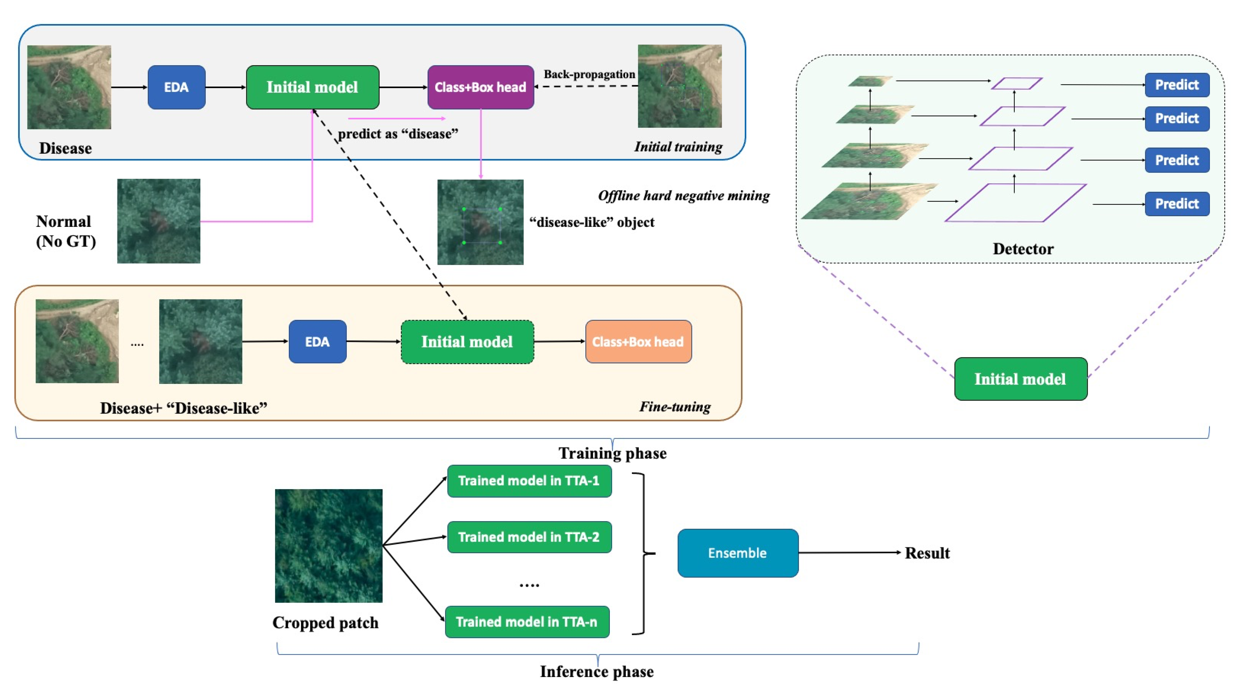
As shown in
Figure 1, we first augmented the training samples with suitable augmentation methods and then trained our first DNN, which was designed to distinguish the background and PWD objects. The detector was robust at detecting most background regions, including healthy trees, land, buildings, lakes, etc., but PWD-infected trees confused with “disease-like” areas (FP) such as yellow land or maple trees. In this phase, it is easy to collect a lot of “disease-like” areas, which is referred to as the mining of hard negative samples [
35]. We further categorized those ambiguous FP samples into six distinct categories (
Figure 2). The disease and “disease-like” samples were passed through the DNN to perform a fine-level object detection. The UAV images in our system included disease regions that varied in size from 12 × 8 to 360 × 300 pixels. Accordingly, we applied a feature pyramid network (FPN) to capture arbitrary scale features based on both bottom-up and top-down connections. ResNet was selected as a backbone network, and the features in each residual block were processed for pyramidal representation. The bottom-up pathway produced the feature map hierarchy and the top-down pathway fused higher resolution features through upsampling the spatially coarse ones. This combined bottom-up and top-down process helps generate semantically stronger features. For the feature maps in each hierarchical stage, we appended a 3 × 3 convolution layer to reduce the aliasing effect of upsampling. Then, the set of merged features of each FPN stage was finally used for predictions. In the inference stage, we cropped the 800 × 800 image patch from the large sized orthophotograph (with “*.tif” extension). We assembled the results of augmented inference images and fused them by weighted boxes fusion algorithm to enhance the location and classification accuracies. A more detailed description of each module is provided later.
3.2. Efficient Data Augmentation (EDA)
Data augmentation is a well-known strategy for significantly increasing the amount of data available for training models without having to collect new data. It acts as a regularizer to reduce bias and generalize the system capability. Real-world UAV images are highly sensitive and collecting them is time-consuming. The image quality of UAV images is dependent on several environmental factors, including reflected light, contrast effects, and camera shake. Meanwhile, detection accuracy is affected by natural weather phenomena such as clouds or thick haze. We used several advanced augmentation methods to improve the performance for locating the PWD in different imaging situations.
Geometric transformation: We first cropped 800 × 800 patches from large “*.tif” images (more than 6 × 10 pixels) and applied random horizontal and vertical flip, rotation (0∼90 degree), and resizing (0.9∼2.0 times zooming) to augment the images and strengthen the model’s ability to handle the various resolutions/shooting angles.
Color space augmentation: The outward appearance of PWD varies based on the stage of the disease; diseased trees are grayish-green in color in the early stage, with the needles turning brown, and eventually ash grey. In the middle stage of the disease, the color of the diseased leaf (brown) resembles the color of a maple leaf. We carried out random gamma, brightness, and contrast adjustments as well as PCA color augmentation [
36] to generate synthetic images from real ones. The trained model with the augmented data including these synthetic images was less sensitive to color and focused more on texture discriminative features.
Noise injection: Poor-quality photography devices mounted on UAV often have unavoidable shot noise from unwanted electrical fluctuation that occurs when taking the pictures. We simulated this condition by adding random Gaussian noise (mean of 0∼0.3, std set to 1) to real images. Moreover, the device can be affected by radio interference, and a damaged image may randomly lose information, where this missing data appears as irregular black blocks. To address this problem, we augmented the training data by adopting the robust regularization technique [
37] (cutout) to randomly remove various regions of input.
Other augmentations: Clouds may block sunlight and create a dark region (shadow) in an image. We added a mask to the original image to change the brightness of the local area of the image so as to simulate shadows. Furthermore, haze is more commonly seen in mountainous areas is another special natural phenomenon that reduces visibility on PWD-infected trees. Changing the opacity of image can generate synthetic haze. We augmented our images to maintain the performance of the network under poor weather conditions.
3.3. The Hard Negative Mining Algorithm
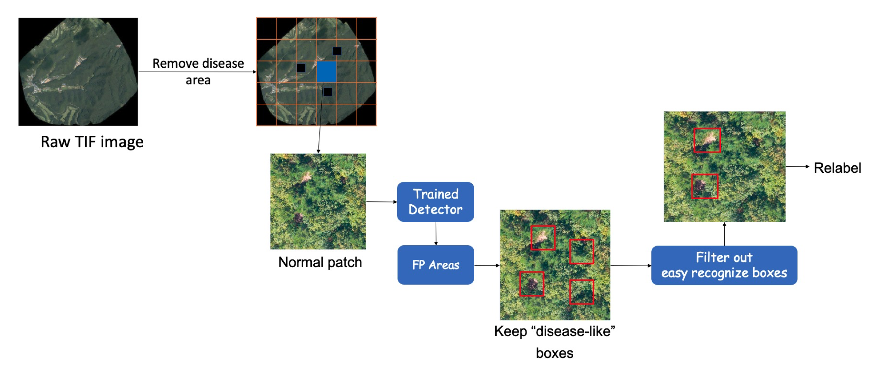
Hard negative mining (HNM) is a bootstrapping method that has been widely used in the classification field and which improves network performance by focusing on hard training samples. We improved the algorithm and applied it to the PWD detection problem. The modified method proceeds according to the following steps: (a) The object detection network is trained on the supervised training dataset. (b) The trained neural network is used to predict the unseen samples (no PWD samples) that are not included in the training samples. (c) The network predicts the objects of interest including “disease-like” objects which can be relabeled into several categories. (d) The “disease-like” objects are merged with genuine PWD-infected objects, and the neural network is retrained on the new dataset. The workflow of selecting “disease-like” objects is shown
Figure 3. Initially, the large-sized orthophotograph (“*.tif”) is divided into small pieces, where the image without GT samples is kept and fed into the trained detector. Then, the model automatically filters out the easily recognizable objects (confidence score < 0.7), and the expert manually relabels the remaining hard objects according to the texture information.
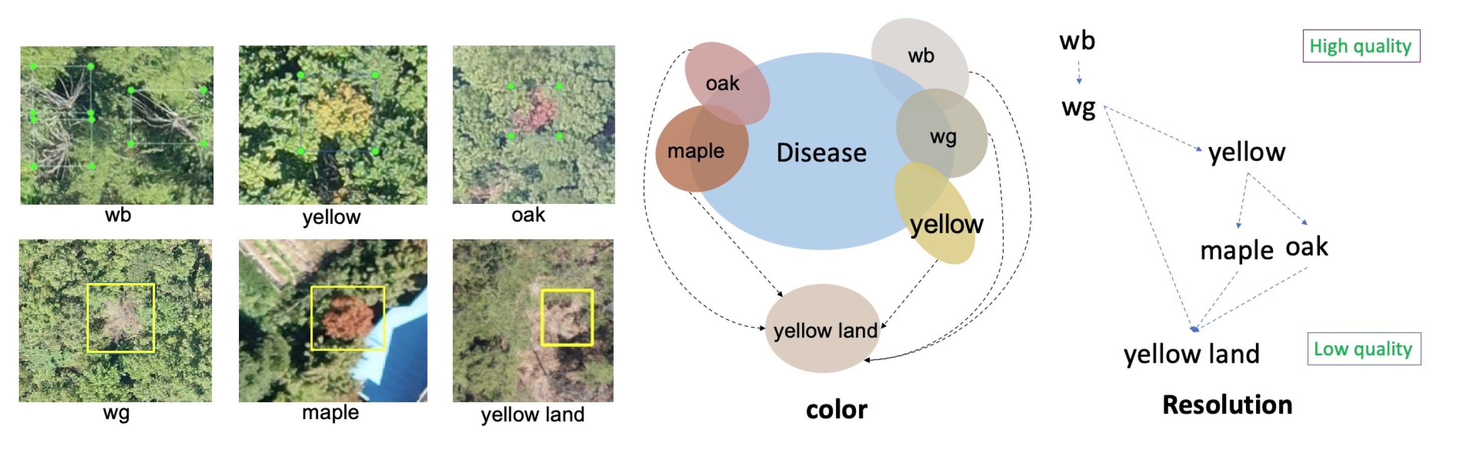
The network with only three categories (background, disease, and hard negative samples) did not perform well due to the ambiguous classification decision boundaries. We manually annotated the hard negative samples into different categories.
Figure 2 shows the division of “disease-like” objects and their relationships with the disease in terms of resolution and color. White branch (wb) denotes a dead tree that has a radial umbrella shape. The white-green (wg), yellow, and maple trees have a homogeneous color similar to PWD in its early and middle stages. The oak category indicates the presence of oak tree disease symptoms that resemble PWD-infected trees in UAV images. We also categorize yellow land into a separate category because this can appear similar to PWD, especially in low-resolution images.
3.4. Test Time Augmentation
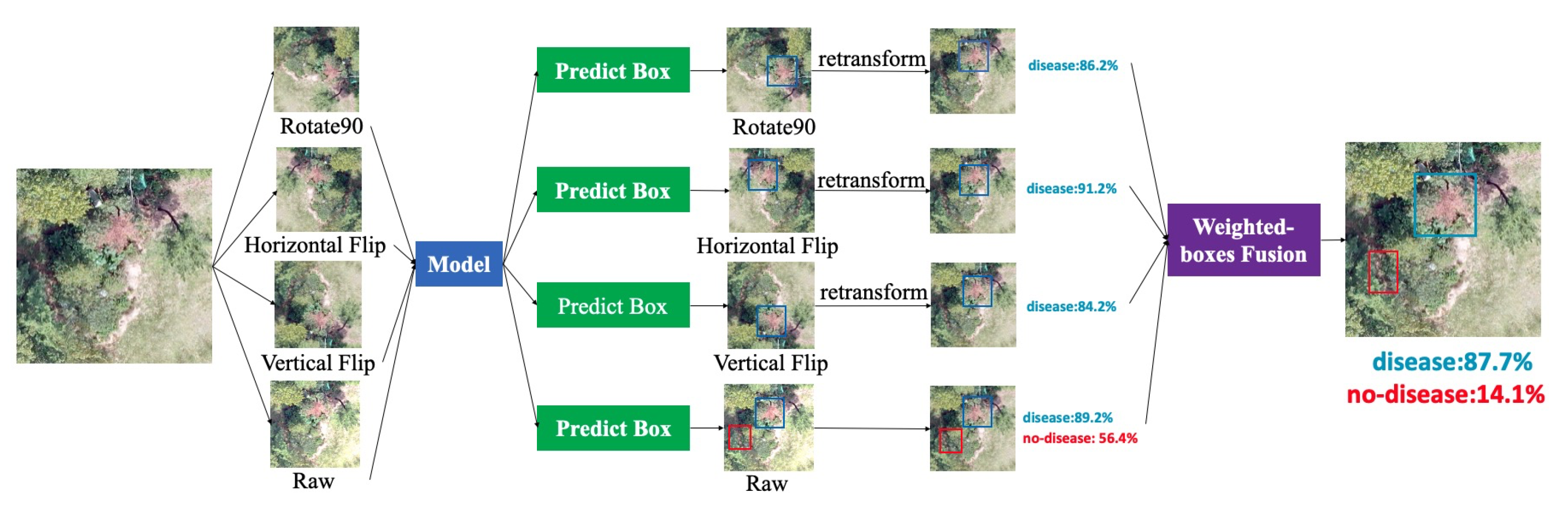
Data augmentation is a common technique for increasing the size of a training dataset and reducing the chances of overfitting. Meanwhile, test time augmentation (TTA) is a data augmentation method applied during test time to improve the prediction capability of a neural network. As shown in the pipeline in
Figure 4, we created multiple augmented copies from a sample image and then made predictions for the original and synthetic samples. The prediction results show the bounding box coordinates with corresponding confidence scores from different augmented samples as well as their original test images. TTA operation is an ensemble method in which multiple augmented samples of a test image are evaluated based on a trained model. The final decision is made by weighted boxes fusion algorithm. While pursuing a balance between computation complexity and performance, we pick three augmentation methods (horizontal flip, vertical flip, and 90-degree rotation) to evaluate the improvement achieved by the TTA method.
3.5. Weighted Boxes Fusion Algorithm
Weighted boxes fusion (WBF) [
38] is a key step while efficiently merging the predict position and the confidence score in TTA. Some common bounding box fusion algorithms such as NMS and soft-NMS [
39] also work well for selecting bounding boxes by removing low-threshold overlapping boxes. However, they fail to consider the importance of different predicted bounding boxes. The WBF method will not discard any bounding boxes; instead, it uses the classification confidence scores of each predicted box to produce a combined predicted rectangle with high quality. The detailed WBF algorithm is described in
Table 2, and the notations used in the table are summarized as follows:
IoU: Intersection over union.
BBox: Bounding box.
N: Augmentation methods (i.e., horizontal flip, vertical flip).
B: Empty list to store predicted boxes from N augmentation methods.
C: Confidence score of predicted boxes.
THR: Mini bounding box overlap threshold.
L: Empty list to save cluster predicted boxes in one position “pos”, “pos” in one position, and IoU of two predicted BBox > THR(largely overlap).
F: Empty list to store fused L boxes in different “pos”.
T: Total number of predicted bounding boxes.
4. Experiment
4.1. Pine Wilt Disease-Infected Image Acquisition
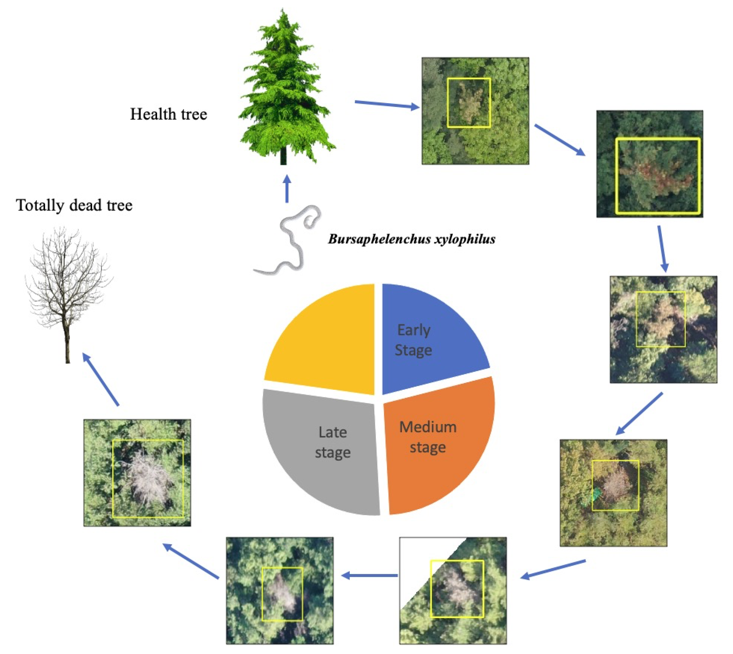
Data acquisition is a primary task in training a robust DNN for classification or regression tasks. For this step, we collected diverse PWD data samples representing various stages of infection, as shown in
Figure 5. Pine wilt can kill a pine tree between 40 days to a few months after infection, and an infected tree shows different symptoms according to its stage of infection. In the early stage, the needles will remain green, but the accumulation of terpenes in xylem tissue results in cavitation, which interrupts water flux in the pine trees. In the second stage, the tree can no longer move water upward, thus causing it to wilt and the needles to turn yellow. The pinewood nematodes then grow in number, and all needles turn yellow-brown or reddish-brown. The disease progresses uniformly branch by branch. After the whole tree is fully dead, the tree needles still remain in place without falling, and show white bare color.
In this work, we obtained UAV images using drone technology. Between August and September, we took orthophotographs with UAVs in the disease-prone region. We tried to capture high-resolution images to best observe the changes in color caused by the disease. We captured high-resolution images from a low altitude using a CMOS camera (Sony Rx R12). The terrain level changes frequently within a hilly region, which affects the resolution quality of an orthophotograph. The images were sequentially taken while overlapping the area. We used drone mapping software (Pixel4Dmapper) to recorrect the GIS coordinates and ensure that the orthophotograph GSD was between 3.2 cm/pixel and 10.2 cm/pixel, where all overlapped patches composed a large orthophotograph (“*.tif”). Furthermore, each large orthophotograph had an ESRI (Environmental Systems Research Institute) format output with geographic coordinates that specify trees that have been deemed to be potentially infected with PWD by experts. During the training, we converted those geographic coordinates to a bounding box annotation. Then, we conducted a large orthophotograph crop to small 800 × 800 patches and sent the data to train the network with GT. After the data cleaning, we obtain a total of 4836 images with 6121 PWD damaged tree points as well as 265,694 normal patches (river, roof, field, etc. no PWD images) used to extract the “disease-like” objects. We used five-fold cross-validation to evaluate our proposed system, where each fold included balanced samples of various resolutions. In the real-world scenarios test, we captured another 10 real-world orthophotographs and compared the results with the expert-labeled ground truth points (730 PWD-infected trees).
4.2. Training Strategy
Our code was written in Python and the network models were implemented with PyTorch. A workstation with multiple TITAN XP GPUs and parallel processing was used to speed up the training. The COCO pre-trained model [
40] was used for transfer learning, and the network was warmed up with a 1.0 × 10
learning rate for the first epoch to reduce the primacy effect. Then, we set a 0.001 learning rate and gradually reduced it by 50% every 50 epochs. In the experiment, the batch size was set to 8, the optimizer was SGD with 0.9 momentum for 200 training epochs. The K-means algorithm [
30] was used to ensure the anchor scales and aspect ratios for fully covering the arbitrary disease shape. We use 5-fold cross-validation to split the training/validation dataset. In the first and second training stages, the strategies were the same except for the difference between the final classification headers. In the first stage, we trained the detection network with two neural nodes (categories) to distinguish between background and PWD-infected trees in the image. In the second stage, we fine-tuned the whole architecture for 200 epochs to distinguish actual PWD damaged trees as well as the other six categories of “disease-like” objects (e.g., wg, maple, wb, etc.).
4.3. Accuracy Estimation
Detector evaluation: We reported the average test accuracy of 5-fold cross-validation. The standard object detection metrics: mean average precision (
mAP) and Recall were used to evaluate the performance of the model, and these are, respectively, expressed as Equations (
1) and (
2).
where
Q is the number of queries in the set and
AP(
q) is the mean of the average precision scores for the given query. Our goal is to identify potential PWD-infected trees as much as possible, and we use Recall as an improvement metric to evaluate how much potential disease area has been located. Recall is assessed as the number of correctly detect diseases (TP) divided by the number of total diseases.
The setup for real-word environment evaluation: Operating in the real-world is even more challenging, as the cropped patches contain not only the PWD-infected trees but also various background content (including “disease-like” objects). Real-world PWD objects are small, irregular, and distributed across a wide area, and the GT is point-wise annotation (x, y geographic coordinates). Converting the point-wise annotation into bounding box annotation is challenging. Our goal was to correctly identify as many disease objects as possible along with their precise positions. In the field investigation to locate the disease-infected tree, an offset error of less than 8 m was deemed acceptable, so we use the x, y geographic coordinates of disease to generate 8 × 8 m GT bounding box annotation for each hotspot. We assume that the disease was found correctly when the overlapped area of GT and predicted bounding box (IoU: Intersection of Union) is larger than 0.3; otherwise, the system prediction is considered to be a false detection.
Specially, we use the overlap strategy to scan the orthophotograph and crop the test patches with 25% overlap. The IoU threshold is set to 0.4 for NMS, and 0.6 for merging the predicted bounding boxes in TTA process. Due to the insufficient context information, FP typically appears on the edge of the test patch. Therefore, we remove the bounding boxes that are less than 5 pixels from the boundary to reduce false alarms; for more information, please refer to
Section 5.1.2.
5. Results
We compared our proposed system to various network architectures.
Table 3 compares the performance of our proposed method to those of alternative structures and backbone networks. The mAP accuracy refers to the average mean of five-fold cross validation in the same hyperparameter setting. We found that FPN with a ResNet101 backbone outperformed other structures, as it obtained the best accuracy of 89.44%; this is attributed to the fact that the fusion of bottom-up and top-down features helps capture disease in an arbitrary shape. The EDA scheme improved system performance as much as 2%. EDA overcomes the issue of data shortages and reduces the environmental effects of imaging. However, other findings were more surprising: the HNM achieved 88.35% accuracy in the FPN + Res101 architecture, and it improved by more than 3% compared to no-HNM approach. This phenomenon also occurs in other structures, which implies that the process in our HNM of splitting “disease-like” objects is important in learning the discriminative features. Another strategy we adopted to improve the inference power was the TTA method. TTA helped eliminate incorrect predictions and boost system performance as much as 1%. The improvement was noticeable in all network structures, as presented in
Table 3. The RetinaNet architecture performed worse than the FPN structure. We suspect that this was caused by the hyperparameters selected in focal loss [
41]. Focal loss has two hyperparameters,
, where
controls the balance of positive and negative samples and
adjusts the weight of learning easy and difficult samples; increasing
makes the model pay more attention to difficult samples. Tuning the two hyperparameter is a challenge task. The goal of this experiment was to evaluate the merit of our proposed strategies, and the results show that they consistently increase the performance of conventional architecture. Further, researchers can apply our proposed strategies in their designed network architectures and obtain better performance. For saving time, For saving time, we used FPN + Res101 structure in the following experiments.
5.1. Result of Real-World Environment Evaluation
5.1.1. Software Integration
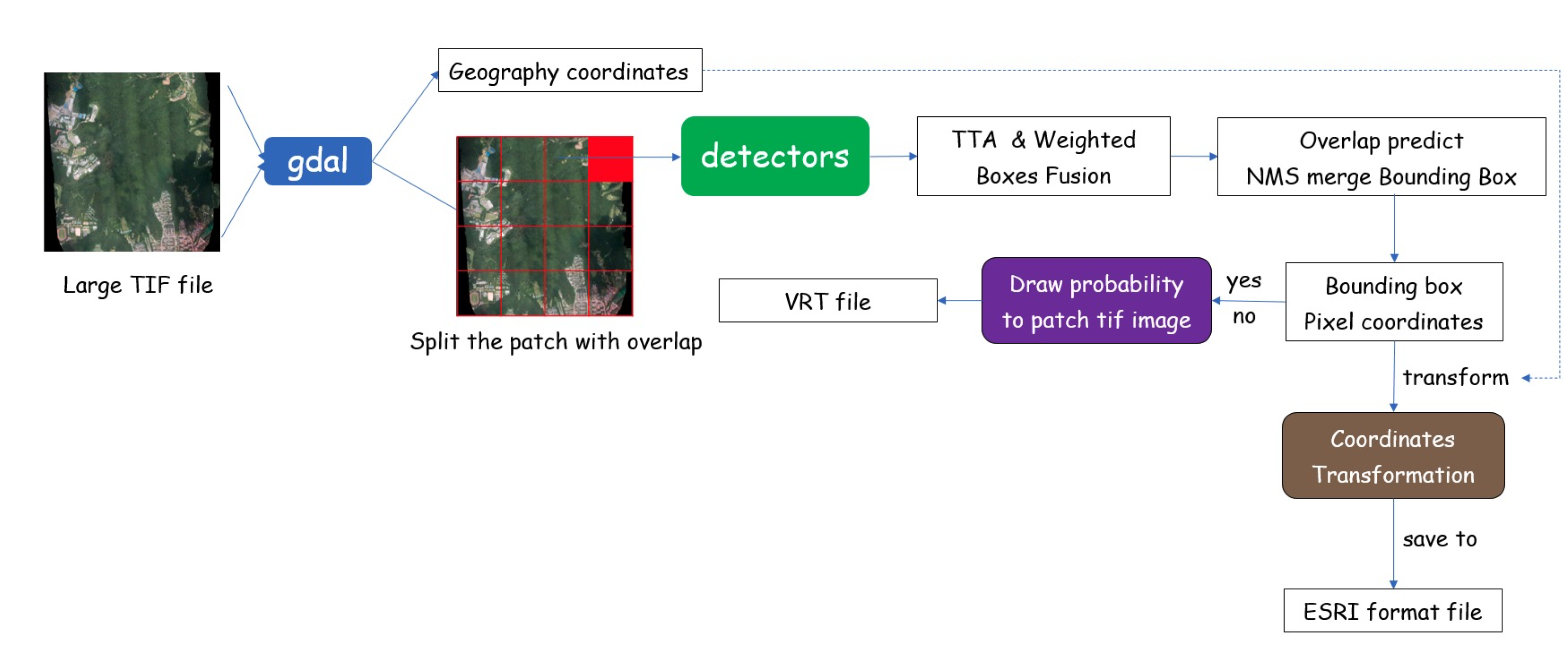
The real-world inference pipeline of our disease detection system is demonstrated in
Figure 6. The UAV with an RGB camera first captured an overlapped image in the survey area. We then processed these images and integrated them into a large orthophotograph. The geographic coordinates are possibly varied due to changes in camera distance, so they had to be carefully recorrected for each object to be kept in its proper position. The resulting 8-bit “*.tif” image was further processed by the GDAL (
https://gdal.org, accessed on 20 December 2021) library and cropped into 800 × 800 patches with overlap. The overlap is essential because the boundary region of the patch has few context information which leads to wrong detection results. We then located the presence of disease in each patch and indicated their location with a bounding box through the inference process.
For each input image patch, we generated augmented patches and returned the combined prediction result from TTA. The models provided the predicted bounding box, which had four points to construct a rectangle: the x and y pixel coordinates for the top left corner as well as the corresponding coordinates for the bottom right corner. Next, we used WBF to select the proper bounding box as well as reduce the number of irrelevant detected boxes in multiple results. After obtaining the precise bounding box location for the disease areas, we transformed the pixel coordinates to geographic coordinates based on the coordinate reference system, and stored the results to an output file. Our program produces the output in ESRI format, which includes four types of files—*.dbf, *.prj, *.shp, *.shx and can be imported into a GIS application for visualization. This application helps experts find the proper GPS coordinates of a potential disease outbreak, and the latitude and longitude information are useful for further field investigation.
5.1.2. The Software Integration Hyperparameter Selection
The selection of proper hyperparameters is critical in the pursuit of better detection software. For real environment evaluations, the important hyperparameters are the stride size, overlap ratio, IoU threshold for NMS, number of augmented methods during TTA, IoU threshold for WBF, and bounding box distance (RBD).
Table 4 lists the hyperparameter settings we used to find potential diseases in Goomisi Goaeup (
Table 5). The stride is the number of pixels that shift over for cropped patches in the next inference time; for example, 3/4 means that, in the next patch, 3/4 pixels (800 × 3/4 = 600) were moved, thus leaving 200 pixels overlapping in the horizontal and vertical directions. The small stride contributes to the increased overlap areas and potentially increases the inference time. RBD refers to the length of the predicted bounding box all the way up to the edge of the cropped patch. The bounding box was removed if the distance between the bounding boxes and the edge of the patch was less than RBD. In our experiment, we obtained a performance improvement of around 7% after removing the bounding boxes near the edge. The reason for this is a lack of context information in the marginal area, which caused the detector to frequently mislabel “disease-like” objects (wg, wb, yellow land, etc.) as disease. Our overlap strategy ensures that there is an overlapped area between the current patch and the next crop patch, so that the next crop patch contains rich context information by removing the bounding boxes located at the edge of the cropping area. Another hyperparameter was the threshold value for NMS. The two-stage object detector needed to generate a large number of candidate bounding boxes to locate the ROI regions, and the NMS was responsible for selecting the best one by filtering out the low confidence scored boxes which have higher IoU values than threshold. The next one was the proper selection of augmented methods in TTA; we used three geometric augmentation methods (horizontal flip, vertical flip, and 90-degree rotation) to evaluate the trade-off between performance and computation complexity. We also tested different IoU thresholds in WBF. In general, we achieved an improvement of 9% by employing proper parameters.
5.1.3. Evaluation in Real-World Dataset
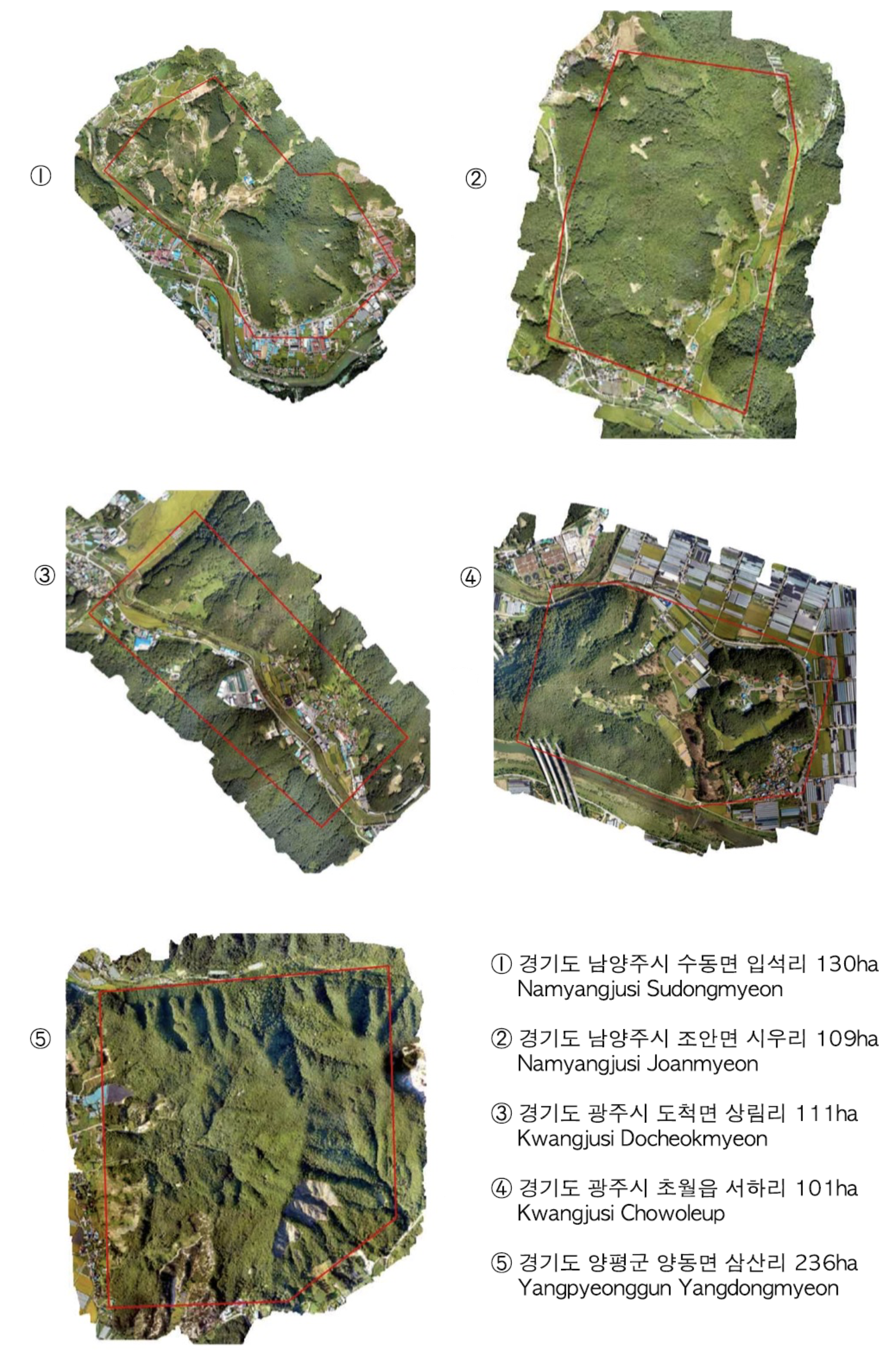
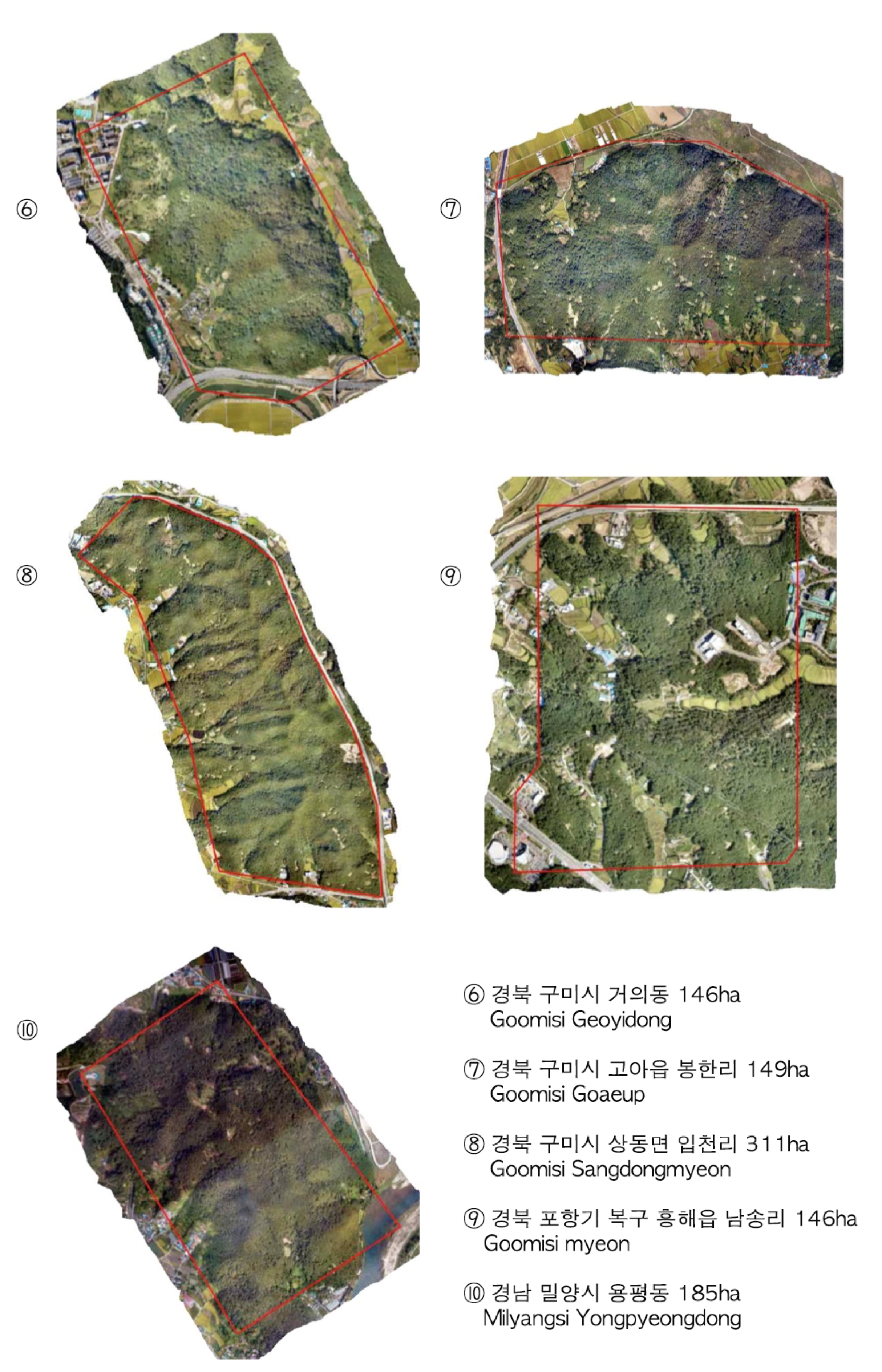
We captured another 10 orthophotographs (
Appendix A) from different cities in South Korea to test the reliability of the proposed system. Each orthophotograph has more than 30,000 × 20,000 pixels (360,000 m
in GSD 6.00 cm/pixel) area (
Table 5). We followed the same preprocessing method as that described in the “software integration” section, and the PWD detector captured 711 out of 730 PWD-infected trees in various resolutions (
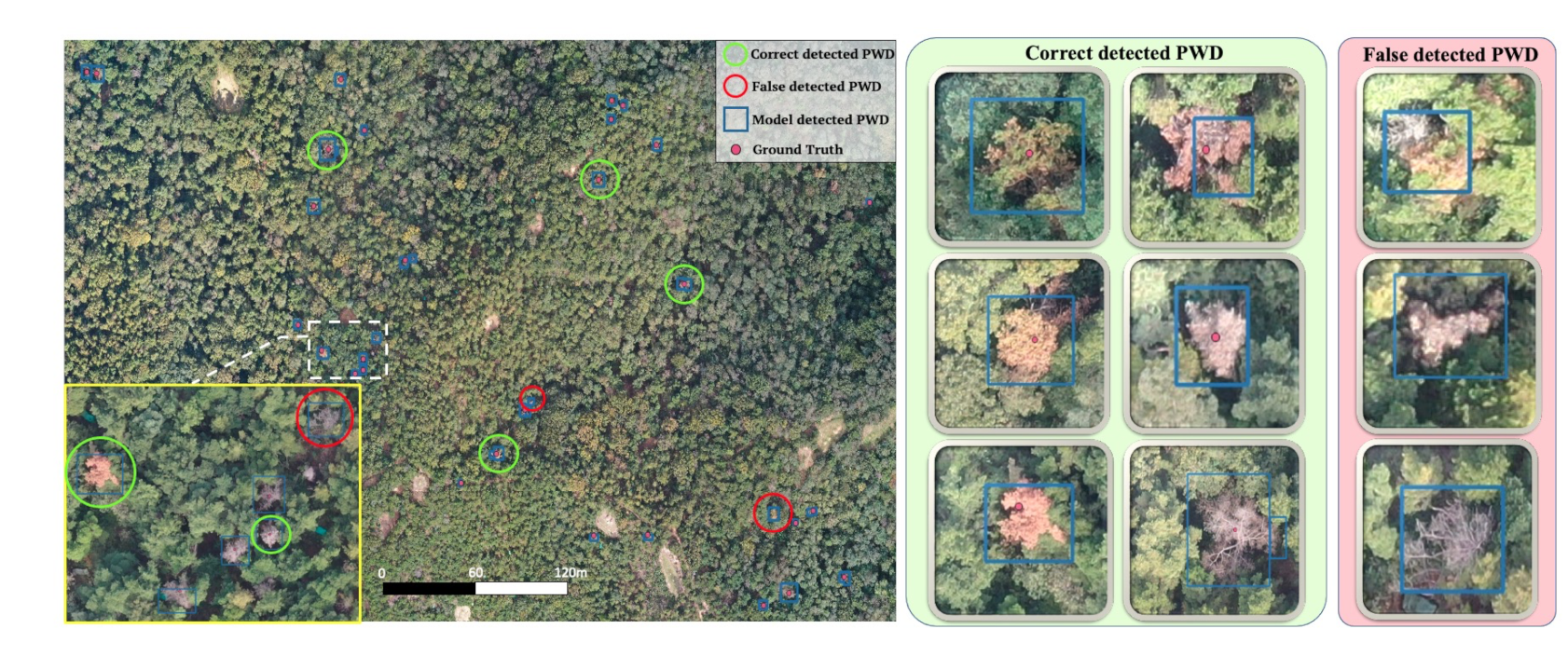
Table 5). To show the robustness of our network, we draw a portion of an orthophotograph in
Figure 7. The potential infected pine trees (GT) are labeled by red dots. The blue bounding box denotes the inference result obtained by the trained detector. The green panel shows the sample of TPs, which has various symptoms of PWD-infected trees across the early to late stage. The red panel shows the false-detected PWD-infected trees. Distinguishing those “disease-like” objects in RGB channels remains a challenging task due to the ambiguity in both shape and color. Further investigations using either multi-spectral images or field investigations are needed.
5.2. The Effect of Hard Negative Mining
HNM was proposed to alleviate the high variance and irreducible error in cases of limited training samples. When the model only sees a few types of disease symptom from a limited number of samples, a large number of background regions makes the detector liable to over-study, whereby it tends to map the true target into no disease. HNM provide many ambiguous “disease-like” objects which share a similar pattern with the disease in the middle and late stages. Including these ambiguous objects helps the model build clear boundaries by learning more discriminative features. In addition, the generated hard negative samples contain a lot of “out of interest regions” (background) such as highways, broadleaf forests, farmland, etc.; this diversity in the training data generalizes the system’s ability to correctly classify real-world problems.
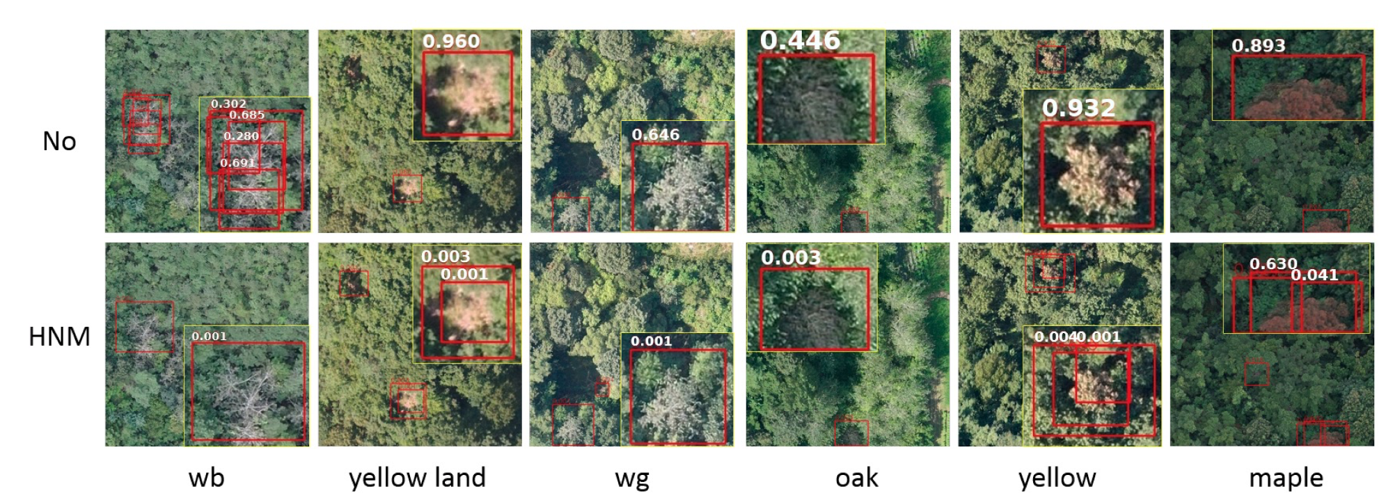
Figure 8 shows some examples of the stark contrast that occurred when we applied finetuning with six “disease-like” categories. HNM successfully suppresses the confidence score of ambiguous objects while locating real disease well. The “wb” category (first column) signifies no PWD-infected dead trees; “wb” and PWD-infected dead trees differ only slightly in the branches. Including “wb” reduces the number of FP bounding boxes and possibly well guides the network to update the network for real PWD-infected dead tree by lowering the confidence score of FPs. Moreover, low-resolution images leads to confusion in identifying the yellow land and small PWD objects. The new category “yellow land” alleviates the effect of ground (confidence score 0.960 –> 0.003 in column (2)). The same phenomenon happens with the “maple” category. Due to the loss of water in the late disease stage, PWD-infected trees tend to show a red-brown color, thus appearing similar to maple trees. Without HNM, the network predicted maple trees (column 6, first row) as PWD-infected disease (high confidence score), but including the additional maple samples promoted the learning ability to filter errors (confidence score 0.893 –> 0.630).
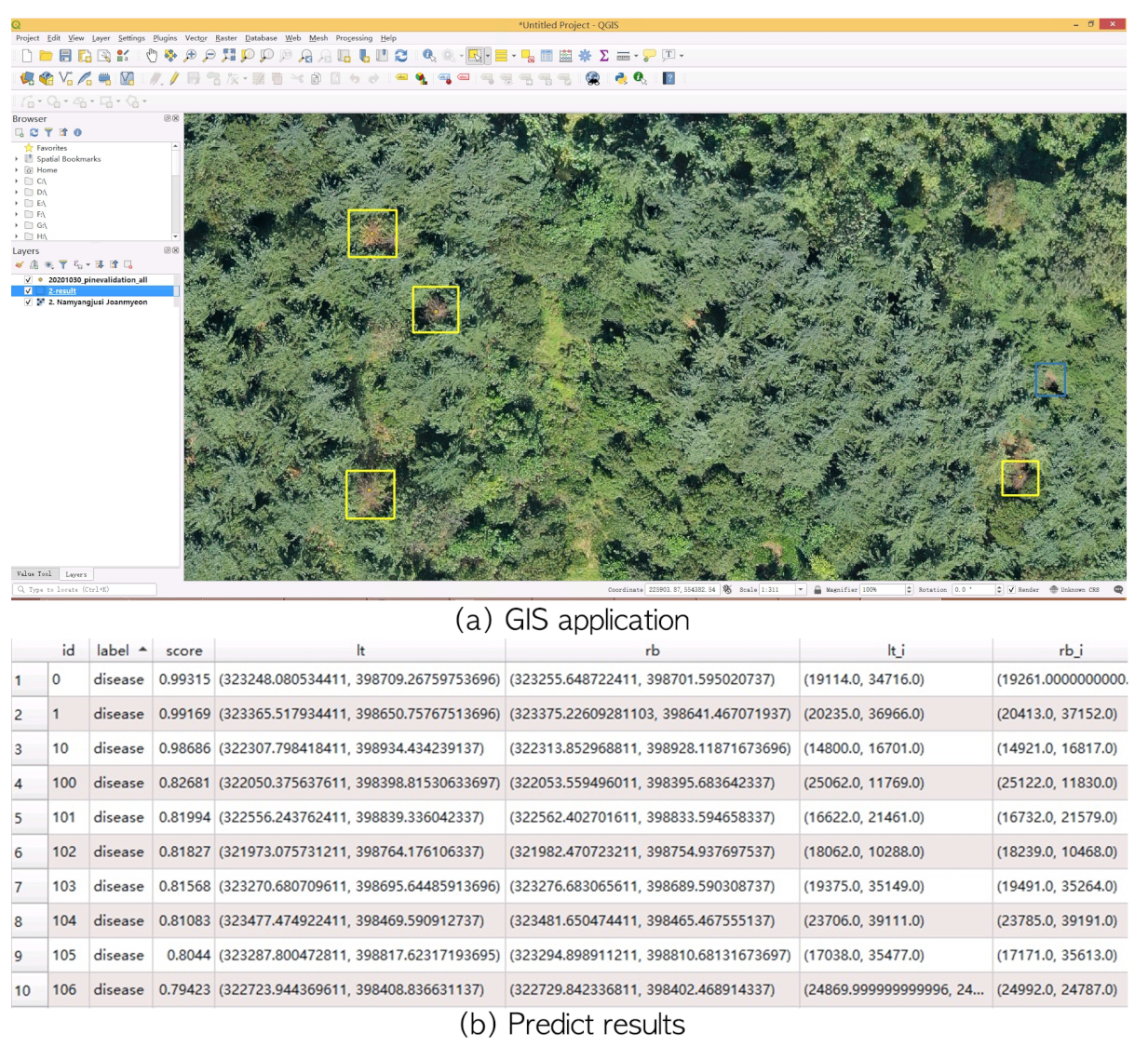
6. GIS Application Visualization
We developed a system with which to process a large orthophotograph (“*.tif”) to predict potential PWD-infected trees, as shown in
Figure 6. The system automatically detects PWD location and saves the location information in standard ESRI format files. The developed system was integrated with QGIS (
https://qgis.org, accessed on 20 December 2021) to visualize the input “*.tif” images and potential disease locations (
Figure 9). Potential disease regions with a high confidence score are represented by yellow bounding boxes while “disease-like” objects are illustrated by blue bounding boxes. The output file preserves class label, predicted confidence score, as well as left-top and right-bottom position for the target bounding box. As shown in
Figure 9b, the column score represents the confidence score within [0,1], and it indicates how much a tree looks like a PWD-infected tree. The expert can reduce the threshold to find more potential disease spots. The columns lr_i and rb_i include the coordinate values of a bounding box in the image coordinate system. The columns lt and rb represent the GPS coordinates in a coordinate reference system [
42] (EPSG: 5186 Korean 2000/Central Belt 2010). Using the lt and rb values, expert can locate PWD-infected trees in field investigation.
7. Discussion and Future Work
In this paper, we proposed a system for improving the performance of the object detection model that detects PWD-infected trees using RGB-based UAV images. To learn a robust network, we created a large dataset which contains a total of 6121 disease spots from various infected stages and areas. The comparison results show that our proposed system has great consistency across different backbone structures. HNM can select “disease-like” objects from six categories. Trained and fine-tuned networks successfully built better decision boundaries with which to distinguish true PWD objects from the six “disease-like” ones. EDA and TTA achieved significant gains by alleviating the data bias problem. In addition, 711 out of 730 PWD-infected trees were identified in 10 large size orthophotographs, indicating that this method shows great potential in locating PWD in various pine forest resources. Finally, the integrated software can automatically locate potential PWD-infected locations and save to ESRI format. It is also convenient to visualize the results in the GIS application for field investigation.
However, there is still work to be done. For example, the best way to utilize context information during the training remains unclear. PWD only infects the pine family, so tree species classification will help reduce inference time and make it easier to precisely locate infected regions. The other problem to be overcome is the method of filtering low-quality images. In UAV images, it is difficult to ensure a consistent resolution, implying that poor-resolution images with ambiguous features decrease the performance. Further, RGB-based PWD detection method still has limitations, as it confuses PWD-infected trees with “disease-like” objects in the early and later stages. Reference [
25] has demonstrated that PWD infected trees exhibit a reduction in normalized difference vegetation index (NDVI), and [
43] showed the effectiveness of conifer broadleaf classification with multi-spectral image. These studies provide insight into the usage of multispectral information to aid in recognition. However, multi-spectral images typically have a lower resolution than RGB images, so the best way to collect and efficiently use multi-spectral images remains a question of interest. We believe our proposed method can be used as preprocessing stage to filter the irrelevant region as well as to find fuzzy PWD hotspot. It is only necessary to reanalyze suspected images with the multi-spectral image, which greatly reduces the time for data collection.


