Abstract
Similar to seasonal and intraseasonal variations in polar motion (PM), interannual variations are also largely caused by changes in the angular momentum of the Earth’s geophysical fluid layers composed of the atmosphere, the oceans, and in-land hydrologic flows (AOH). Not only are inland freshwater systems crucial for interannual PM fluctuations, but so are atmospheric surface pressures and winds, oceanic currents, and ocean bottom pressures. However, the relationship between observed geodetic PM excitations and hydro-atmospheric models has not yet been determined. This is due to defects in geophysical models and the partial knowledge of atmosphere–ocean coupling and hydrological processes. Therefore, this study provides an analysis of the fluctuations of PM excitations for equatorial geophysical components χ1 and χ2 at interannual time scales. The geophysical excitations were determined from different sources, including atmospheric, ocean models, Gravity Recovery and Climate Experiment (GRACE) and GRACE Follow-On data, as well as from the Land Surface Discharge Model. The Multi Singular Spectrum Analysis method was applied to retain interannual variations in χ1 and χ2 components. None of the considered mass and motion terms studied for the different atmospheric and ocean models were found to have a negligible effect on interannual PM. These variables, derived from different Atmospheric Angular Momentum (AAM) and Oceanic Angular Momentum (OAM) models, differ from each other. Adding hydrologic considerations to the coupling of AAM and OAM excitations was found to provide benefits for achieving more consistent interannual geodetic budgets, but none of the AOH combinations fully explained the total observed PM excitations.
1. Introduction
Variations in the Earth’s rotation, in relation to the crust of our planet, is commonly expressed by the term polar motion (PM). Such rotations are mainly governed by the redistribution of masses and their motion within surficial fluid layers. These masses are composed of the atmosphere, the oceans, and inland freshwater systems including snow, ice, and soil moisture and ground water flows. Angular momentum exchanges between the Earth’s core and the mantle are also responsible for rotation variations.
Apart from external torques from the luni-solar tides, PM variations change on all observable timescales, from sub-daily to decadal and beyond, caused by interactions among different components of the Earth’s system. Variations in the distribution of mass within the geophysical fluid layers that produce fluctuations in PM components of the angular momentum of the Earth, particular for interannual timescales, are the subject of the present study.
The common approach for studying the polar motion is to compare the geodetic excitation GAM with the geophysical excitation mostly reconstructed from models of the global circulation taking place in the hydro-atmosphere. Effective angular momentum (EAM) functions summarize the excitation of Earth orientation changes due to atmosphere, ocean, and the land hydrosphere. The equatorial EAM components χ1 and χ2 excite PM, and the axial component χ3 quantifies UT1. The International Earth Rotation and Reference Systems Service (IERS; https://www.iers.org/IERS/EN/DataProducts/GeophysicalFluidsData/geoFluids.html, accessed on 15 November 2021) provides a comprehensive list of publicly available model-based EAM for the atmosphere (AAM), ocean (OAM), and terrestrial water (HAM). A number of previous studies analyzed, compared, or even combined such EAM data sets in detail (e.g., [1,2,3,4,5,6]).
Past studies have shown that Atmospheric Angular Momentum (AAM) and Oceanic Angular Momentum (OAM) are dominant contributors to PM excitations in broad frequency bands [1,2,3,4,5,6]. Additionally, Glacial Isostatic Adjustment (GIA) is a dominant contributor for linear PM trends (e.g., [7,8]). Recent results suggest that mass redistributions in the hydrological and cryosphere systems can also excite interannual PM (e.g., [9,10,11]). In particular, the potential of GRACE (Gravity Recovery and Climate Experiment) data to study interannual Terrestrial Water Storage (TWS) changes on a global scale and its impact on PM has been demonstrated [10]. A positive correlation between complex geophysical and geodetic components was observed. A comprehensive analysis of interannual oscillations in all three axes of the Earth’s rotation using accurately measured PM and length-of-day time series and geophysical excitations has been examined previously [12]. In addition, oscillations with periods of around 5.9, 3.65, and 2.5 years caused by hydro-atmospheric excitations were identified.
To study interannual variations in PM, the MSSA method can be employed to improve decompositions of geodetic and geophysical excitations of PM into various reconstruction components (RC). MSSA is a non-parametric analysis technique for non-linear time series, also called Extended EOF. This method is a generalization of Singular Spectrum Analysis (SSA) for multidimensional time series [13,14]. Over the last two decades, the MSSA method has been widely used in the identification of periodic or modulated oscillations in geophysical and climatic time series [15,16,17]. Recently, this technique has been used for PM analysis changes, as well as its prediction [18,19]. The MSSA method decomposes the time-delayed embedding of a given dataset [20,21] into a set of data-adaptive orthogonal components, and takes cross correlations into account as well. These components can be classified into trends, oscillatory patterns, and noise, and permit the reconstruction of a time series demonstrating the underlying dynamic system structure [17,22].
Therefore, the main objective of this paper is to assess the agreement between observed Geodetic Angular Momentum (GAM) and geophysical excitations at interannual time scales using data from different processing centers. To achieve this, the importance of different AAM and OAM model combinations was explored, along with their mass and motion components. Moreover, the potential improvements to PM analysis as a result of using different gravimetric hydrological excitations were discussed as well.
2. Data and Methodology
This study provides a comprehensive analysis of monthly interannual oscillations in PM components using accurately measured PM time series, and geophysical excitations computed from atmospheric, oceanic, and hydrological models between October 2002 and October 2019. Specifically, the GRACE and GRACE Follow-On data are tested here to confirm the interannual oscillations remaining in PM after detrending and band-pass filtering using MSSA decomposition to retain variations at periods between 1.5 and 8 years.
2.1. Earth Orientation Parameters
In this study GAM was obtained from the International Rotation and Reference System Service (IERS), where the earth orientation parameters x, and y pole with respect to IAU 2006/2000A precession-nutation model and consistent with International Terrestrial Reference Frame (ITRF2014), the so called EOP 14 C04 (IAU2000A) time series was used [23]. This series is derived from a combination of different space geodetic techniques. Daily observed PM excitations were computed from the C04 series using the IERS online tool (http://hpiers.obspm.fr/eop-pc/index.php?index=excitactive&lang=en, accessed on 16 November 2021) with a Chandler period of 433 days. Geodetic equatorial, χ1 and χ2, excitation functions are computed using the Liouville algorithm (e.g., [24]):
with pole coordinates and complex Chandler frequency , with a Chandler period days and a damping Q = 100.
2.2. Geophysical Excitation Functions for Polar Motion
PM excitations can be studied by applying the principle of angular momentum conservation to the fluid layers of the Earth’s system (e.g., [25,26,27]). The Effective Angular Momentum Functions (EAMF) relate changes in angular momentum to PM excitations and consist of two terms, one referred to matter, and the other to motion (e.g., [28]). The matter term ( describes the influence of mass redistribution on the Earth’s inertia tensor, while the motion term corresponds to the relative angular momentum change with respect to the mean rotating reference system (e.g., [29]):
where the Earth’s inertia tensor is expressed as and the relative angular momentum is expressed as . Meanwhile, is the mean angular velocity of the Earth, is the axial principal moment of inertia, and is the mean equatorial principal moment of inertia. The factors 0.684 and 1.608 account for the yielding of the solid Earth to surface mass loading and the effect of core decoupling, respectively. Numerical values for these factors are taken from [24].
In this study, different equatorial EAMFs computed from different sources are used to describe the geophysical excitation functions of PM and assess the ability of these models to explain full interannual signals in geodetic observations.
Here, we focus on interannual signals (periods between 1.5 and 8 years) from the atmosphere, oceans, and land hydrologic systems. By working in the time and frequency domain, interannual PM signals from geodetic and geophysical excitations from the atmosphere + ocean (AO) time series were compared. These readings were improved by PM hydrological excitations computed from different sources. The first AO combination was calculated based on the National Centre for Environmental Prediction/National Centre for Atmospheric Research (NCEP/NCAR) data for AAM and ECCO kf080 data for OAM. The second combination was obtained from the Earth System Modeling models of AAM and OAM provided by the GeoForschungsZentrum scientific group [4]. To consider the aforementioned hydrological effects on interannual PM variations, shown to be significant in [10], Hydrological Angular Momentum (HAM) series were taken into consideration from four sources. Special attention was paid to global mass balance effects, which is important for geophysical interpretations of PM and crucial for day length variations [5,29,30]. Moreover, interannual signal interpretation by geophysical excitations in PM is only valid if the total observed excitations, along with the hydro-atmosphere models, are free of errors. However, current geophysical fluids models generally do not properly clarify the total mass in the atmosphere, oceans, and terrestrial hydrology and cryosphere systems, which is one of the largest current error sources for quantifying the so called “geodetic budget”. The effect of global mass conservation among different model combinations has been often neglected, most likely due to the absence of adequate data products. In this study, the so called barystatic Sea-Level Angular Momentum function (SLAM) that account for the global mass balance consistent to their models used for the calculation of AAM, OAM, and HAM products [4] provided and publicly available on the Earth System Modelling group at GFZ Potsdam (ESMGFZ) is used.
Except for the model errors and effect of global mass conservation, the accuracy of measurement of PM, which is uniquely well observed at the level of roughly 1 mm of surface rotation [31], also has an impact on the agreement between GAM and AO excitations.
Two coupled AO time series (AO1 = NCEP/NCAR + ECCO, and AO2 = ECMWF + MPIOM) are examined here to indicate which one better represents the full geophysical changes at interannual PM excitations.
2.2.1. Polar Motion Atmospheric and Oceanic Excitations
PM AAM was computed from the National Centre for Environmental Prediction/National Centre for Atmospheric Research (NCEP/NCAR) re-analysis model [32], provided by the Special Bureau for the Atmosphere of the Global Geophysical Fluids Center (GGFC) [33]. The NCEP/NCAR re-analysis model covers the years from 1948 to present. Each component of the AAM NCEP/NCAR time series consists of a pressure term (), due to air mass redistribution, and a wind term (), due to atmospheric relative angular momentum [34]. Atmospheric pressure excitations are computed from daily surface pressure fields, considering the inverted barometer (IB) assumption for oceans; assuming that oceans respond to the atmospheric loading isostatically. These equatorial AAM time series have a sub-daily sampling period equal to 6 hours.
PM ocean excitations include contributions from both ocean currents and ocean bottom pressure variations [35]. The non-tidal oceanic PM excitation is expressed by an OAM series estimated from the ECCO kf080 model run at the Jet Propulsion Laboratory [36]. It considers atmospheric surface wind stresses, temperatures, and freshwater fluxes taken from the output fields of the NCEP/NCAR reanalysis [37]. The data series, which are available from the IERS Special Bureau for the Oceans, contains daily values of equatorial OAM due to currents and ocean bottom pressures from January 1993 to August 2020 [38].
In addition, a consistent set of geophysical excitations of AAM, OAM, and HAM, were used in this study. The Earth System Modeling group at GFZ (ESMGFZ) routinely provides the EAMF describing the nontidal geophysical excitations of the Earth’s orientation changes due to mass redistribution and the atmosphere’s relative motion [39]. The temporal resolution of the ESMGFZ AAM have a 3 h sampling. Tidal variations for the 12 most relevant frequencies are fitted and removed by ESMGFZ from the data to retain the nontidal signal only [40]. Daily updated ESMGFZ AAM functions are calculated from numerical weather model data provided by the ECMWF. The IB correction is applied to surface pressures from all oceanic locations of the underlying grid [41]. OAM time series are calculated from the ocean bottom pressures and ocean currents of an unconstrained simulation by the Max Planck Institute from the Meteorology Ocean Model (MPIOM; [42]). The OAM MPIOM ocean model is calculated with the same atmospheric data from the ECMWF model that was used for AAM. The IB correction is also applied to ocean bottom pressures, and the oceanic response to atmospheric tides is estimated and removed from both mass and motion terms. OAM are available with the same temporal sampling and at the same frequency as the AAM from ESMGFZ.
2.2.2. Polar Motion Hydrological Excitations from Models and GRACE Data
To improve the agreement between the observed geodetic time series, GAM, and geophysical excitations, different PM hydrological excitation functions (considering HAM) were summed to different AAM and OAM excitation models.
The EAMF calculated from terrestrial water storage was simulated with the Land Surface Discharge Model (LSDM). Terrestrial water storage changes include snow accumulation, seasonal runoff from glaciers, and water flow in river channels given daily on a regular global grid. The hydrological discharge model (HDM; [43]) and Simplified Land Surface Scheme (SLS; [44]) were used to define the physics and parametrization of the LSDM discharge model. Similarly, for the AAM and OAM models of ESMGFZ, the LSDM hydrological model was calculated with atmospheric data at high spatial and temporal resolution obtained from the corresponding ECMWF models. Additionally, barystatic sea-level changes (SLAM) were added to the HAM LSDM hydrological excitation time series. Thus, the effect of SLAM balances the global mass in the model, stabilizing the sum of total masses in all different effective angular momentum components (AAM, OAM, HAM, and SLAM).
Since 2002, the Gravity Recovery and Climate Experiment (GRACE) satellite mission, and its successor GRACE Follow On, have monitored global mass redistributions with an unprecedented accuracy. As a consequence, GRACE provides new types of data, giving a large quantity of data for terrestrial water storage changes over land areas. In this study both level-2 and level-3 data from GRACE/GRACE FO satellites are used to calculate mass terms for HAM excitations.
Level-2 GRACE/GRACE-FO datasets are expressed as spherical harmonic geopotential coefficients with a specified maximum degree and order. Nonetheless, for the study of PM excitations, only degree-2 order-1 (ΔC21, ΔS21) coefficients are needed. The changes in χ1 and χ2 equatorial components of HAM are proportional to the variations in ΔC21 and ΔS21, which permits the calculation of HAM independently from other coefficients [45]. The relationship between the complex equatorial components of HAM and spherical harmonics coefficients ΔC21, ΔS21 of geopotential is described in [29].
It should be noted, that PM hydrological excitations computed from the Level-2 Grace Satellite only Model (GSM) coefficients, mainly contain hydrological and cryospheric signals since the atmospheric and oceanic impacts (Atmosphere and Ocean De-Aliasing Level-1B Release-6 or AOD1B RL06) are removed in all GRACE/GRACE-FO datasets [46]. The residual ocean signals retained in HAM excitations computed from GSM may be due to the non-removal of the entire mass of oceans, errors in the ocean model used to determine AOD1B, and leakage between land and ocean. In addition, hydrological excitations computed from ΔC21 and ΔS21 coefficients contain signals from post-glacial rebound, barystatic sea-level changes, contributions resulting from inflow of water from land into oceans (so-called sea-level angular momentum or SLAM) or tectonic events related to large earthquakes [9].
The GRACE/GRACE-FO Level-3 data, in the form of spherical harmonics, is based on TWS, and mass concentration solutions (called “mascons” or MAS) from Release-06 version 2 data from the Center for Space Research (CSR) at the University of Texas at Austin. This level-3 data was also used to improve interannual geophysical signals. TWS anomalies are given in regular latitude–longitude grids and are obtained from spherical harmonics (SH) coefficients of all available degrees and orders, after appropriate reprocessing (filtering, correcting due to glacial isostatic adjustment (GIA), replacing ΔC20 coefficient with an estimate from SLR, and correcting degree-1 coefficients). These products provide information on changes in the water content in terrestrial areas only because of the masking of ocean regions. Consequently, the resulting HAM excitations series describe the effects from continental water, snow, and ice without residual ocean signals, or barystatic sea-level changes. Like gridded TWS anomalies, MAS represents GRACE/GRACE-FO Level-3 data, delivering monthly changes of TWS. Unlike GSM data and gridded TWS anomalies, MAS models do not use spherical harmonic functions but instead apply mass concentration functions. The MAS approach also enables better separation of land and ocean signals than the SH approach. HAM excitations series obtained from MAS data only express the impact of land hydrosphere, snow, and ice on PM excitation because it masks the ocean areas. The GRACE Level-3 data includes corrections, filtering, and the removal of atmospheric mass/pressure changes (based on the ECMWF model), GIA, truncation of SH coefficients at 60 degrees, and the application of a destriping filter alongside a 300 km Gaussian smoother. Hydrological excitation functions computed from GRACE CSR RL06M v02 data should mainly represent variations in χ1 and χ2 equatorial components of PM due to the redistribution of continental water.
Other solutions for TWS components computed from other centers (JPL, GFZ) also exist. In principle, some differences in these different solutions are discussed in [9]. Furthermore, in the paper [47] a detailed description of the different GRACE/GRACE-FO products and their HAM solutions in exciting PM is shown. In this study, the GRACE CSR RL06 from GSM, TWS, and MAS were selected in order to assess their ability to improve geophysical signal in PM excitation.
2.3. Multi-Channel Singular Spectrum Analysis
The equatorial geodetic and geophysical excitation function is expressed through complex components, so two channels were selected for the analysis. It is assumed that the observed GAM and geophysical AO1 and AO2 time series, in and components, are and channels describing time and length , respectively.
The main parameter of the method is lag . There are several recommendations for the window size of , which usually meets the criterion of [48]. To better extract the periodic terms, is the multiple of periods of the expected oscillations. Seasonal, especially annual periods are a reasonable choice for the GAM, AO1, AO2, and HAM time series periods. In this study, is chosen as the window size, which is equal to 6 years (the time series interpolated to a 30.4-day time step).
The first step of the MSSA algorithm is to compute the trajectory matrix , which contains all considered channels (in this study there were two channels, and , for each equatorial component of geodetic and geophysical excitation functions) [49]:
Then, the multichannel trajectory matrix is computed as:
where is a number of time series in the analysis and is equal to 2 (considering the and excitation components).
In the next step, the grand lag-covariance matrix Y is computed using the BK (Broomhead and King) equation [20]:
Then, the grand-lag covariance matrix is decomposed by singular value decomposition [50] in order to compute the eigenvalues and eigenvectors related to empirical orthogonal function (EOF).
Projecting the augmented trajectory matrix onto the eigenbasis , given by , whose columns are the associated eigenvectors , yields the corresponding Principal Components (PC), as columns of matrix .
The k-th reconstructed component (RC) at time t for time series l is defined as [51]:
Depending on the frequency that is extracted from the time series, various components can be reconstructed. It is worth emphasizing that summing all RCs, the original time series is reconstructed with no loss of information.
3. Results
The purpose of this study was to evaluate ability of geophysical excitation functions calculated from different models and GRACE data to close the “geodetic budget”: at interannual time scales. GAM fully represents geodetic PM excitations. Geophysical excitation functions (AO2, HAM, and SLAM) from atmosphere–hydrosphere models are coupled through a global mass balance constraint. In AO1 combination, the OAM ECCO is forced by AAM NCEP/NCAR model. HAM is the hydrological portion computed from the Terrestrial Water Storage redistribution of land freshwater from different representations of GRACE solutions: Stokes coefficients, TWS and mass concentrations.
In the first part of the analysis, the quality of original geophysical fluid models, AO1 = AAM NCEP/NCAR + OAM ECCO kf080 and AO2 = AAM ECMWF + OAM MPIOM, on interannual observed geodetic PM is evaluated, considering both mass and motion. In the second part of the analysis, interannual geophysical excitations are improved by hydrological PM excitations via the LSDM model and by gravimetric-hydrological PM excitations computed from different GRACE and GRACE Follow-On solutions from the Center for Space Research.
All geodetic and geophysical time series were interpolated with a monthly time span in order to maintain an equal time span for GRACE and GRACE Follow-On gravimetric time series. In addition, a one-year gap (6/2017–6/2018) between GRACE and GRACE Follow-on gravimetric excitation functions was filled by performance forecasting using the seasonal ARIMA method, with the arima function available in Matlab.
Figure 1a shows the observed GAM seasonal oscillations for and equatorial components of PM, extracted using the MSSA method. From all reconstructed time series, those were chosen whose spectrum gave a frequency between 1 and 3 cycles/year from the fast Fourier transform. The amplitudes of these reconstructed components varied in time, and in general decreased since 2012, for both the and components. Seasonal variations in PM are relatively stable, and its amplitude varies between 10–20 mas and 20–50 mas in and respectively. This variety may reflect that the seasonal redistribution of the mass of Earth, which has good stability, is changing over time. These changing seasonal terms may be a combination of multiple other periodic terms, and thus only represent a mathematical expression of MSSA, and further research and analysis are needed. Interannual time series were computed as the sum of the reconstructed components with the frequency above 1.5 cycles per year (Figure 1b). The sum of seasonal and interannual GAM excitations, extracted by the MSSA method, explain PM oscillations in and , in and , respectively (Figure 1c). Similarly, monthly AO1 and AO2 excitations were decomposed by the MSSA method into seasonal and interannual components for and (Figure 2a,b). Some discrepancies between atmosphere–ocean models were observed, especially in PM seasonal components. The sum of interannual and seasonal components of geophysical excitations AO1, and AO2 extracted by the MSSA method, explain about and of the total geophysical excitations for the and equatorial components (see Figure 2c,d).
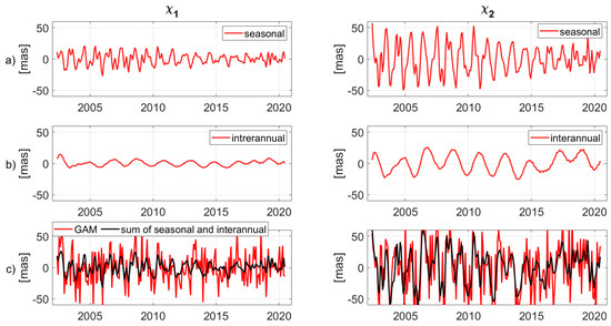
Figure 1.
Monthly excitations of polar motion (GAM) per reconstruction parameters (RCs) forMonthly excitations of polar motion (GAM) per reconstruction parameters (RCs) for and equatorial components of (a) seasonal, (b) interannual, and (c) overall vs. sum of seasonal and interannual oscillations.
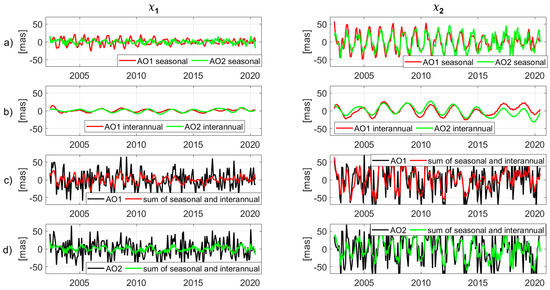
Figure 2.
Monthly geophysical PM excitations (AO1, AO2) per reconstruction components (RCs) for and for (a) seasonal, (b) interannual intervals, plus (c) AO1 overall vs the sum of seasonal and interannual oscillations of AO1, (d) AO2 overall vs. the sum of seasonal and interannual oscillations of AO2 excitations.
In the next part of this study, special attention was paid to the interannual oscillations only. Seasonal parts of GAM and AO excitations were shown as an example of the possibilities of the MSSA method to decompose time series into different spectral bands. In addition, it should be noted that the sum of all the reconstructed components added up to and matched the original time series.
3.1. Geodetic Excitations from Different AAM and OAM Models
Figure 3 compares the observed GAM, along with different combinations of geophysical components of mass and motion for the monthly interannual and time series excitations from 10/2002 to 10/2019. From Figure 3a, the NCEP/NCAR and ECMWF mass components of atmospheric excitations are very similar, both in and components. Their root mean square (RMS) values, presented in Table 1, differ by and mas, for and , respectively. Meanwhile, adding the mass components to the motion term for both AAM models (see Figure 3b), the AAM NCEP/NCAR, and AAM ECMWF time series were found to differ from each other. Despite this, the interannual AAM time series of the total mass and motion terms explain GAM better, than using only the AAM mass term.
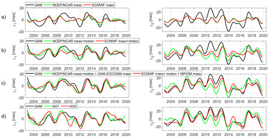
Figure 3.
(a) Monthly interannual excitations of geodetic GAM excitations and different combinations of geophysical mass and motion terms of and components (AO1, AO2): (b) GAM vs. AAM NCEP/NCAR and AAM ECMWF of their mass components, (b) GAM vs AAM NCEP/NCAR and AAM ECMWF of their mass + motion components, (c) GAM vs. AAM NCEP/NCARmass+motion + OAM ECCO 080mass and AAM ECMWFmass+motion + OAM MPIOMmass components, (d) GAM vs. AO1 = NCEP/NCARmass+motion + OAM ECCO 080mass+motion, and AO2 = AAM ECMWFmass+motion + OAM MPIOMmass+motion geophysical excitations.

Table 1.
RMS of the GAM interannual excitations and of the different interannual mass and motion terms of geophysical excitations from different models.
Discrepancies between the monthly interannual AAM NCEP/NCAR and AAM ECMWF motion time series are significant, where the RMS differences in the component reach the value of mas, where they are greater than the components and equal mas. In the case of the NCEP/NCAR atmospheric model, it was shown that wind is the single most important contributor to , which was also found in previous studies [10], but which is not considered in the AAM ECMWF model.
Adding the oceanic bottom pressures to AAM excitations improved the agreement between GAM and geophysical fluid models (see Figure 3c). The agreement at interannual time scales is bigger for the component of PM than for . The total influence of monthly interannual geophysical fluid excitations, containing the impact of atmospheric winds, surface pressure, oceanic currents, and ocean bottom pressures for different combinations of NCEP/NCAR, ECMWF, ECCO kf080 and MPIOM models on PM is shown in Figure 3d. From visual inspection, both AO1 and AO2 geophysical models are far from being perfect in completely explaining the observed interannual geodetic PM changes; although, their variability is closest to GAM excitations. The RMS value of differences between GAM and AO excitations indicate, that the interannual signal is not fully explain by atmosphere and oceans. Furthermore, AO2 combination better reduce geophysical signal in PM excitation in component. Both, AO1 and AO2 excitations of χ1 component reduce the GAM excitations on the similar level. This observation is also confirmed by the results in Table 1 that lists the RMS of the AO1, AO2, GAM, and GAM-AO time series.
Successively, adding the mass and motion terms of AAM and OAM provided a better correlation with the GAM time series, but did not entirely account for the interannual variations. Additionally, it did not help to select which combination, AO1 or AO2, is a better representation for PM geophysical contributions.
Figure 4 shows the correlation coefficients between observed geodetic PM time series and different geophysical excitations, starting with the mass terms for AAM and OAM, and successively adding the motion parts of AAM and OAM for both for AO1 and AO2. Rates of explained variance for GAM signals, in and components, are also shown in Figure 4. The explained variance rate of the series and is defined by:
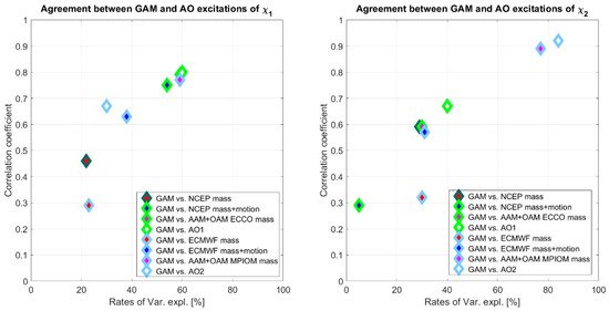
Figure 4.
Correlation coefficients and rates of explained variance between geodetic and geophysical components of mass and motion terms and their combinations of interannual PM excitations, for (left panel), and (right panel).
If perfectly accounts for , the standard deviation of the difference is and so the .
For identical time series, rates of variance equaled , and for time series not fitting at all it might be even negative. For equatorial components, a better correspondence of AO2 series with the observed GAM excitations was found, over AO1 excitations, whose rates of explained variance reached , and the correlation coefficient was equal to 0.92 (the highest among all the considered geophysical excitations). However, the agreement between GAM and AO1 excitations for was better than for AO2 excitations. Compared to the RMS of full excitations, both the matter and motion terms of the atmospheric and oceanic effects are important and have different impacts on interannual PM excitations. Despite these promising results, it was not possible to find a conclusive indication of which combination of AAM and OAM is the best to explain GAM excitations.
3.2. Geodetic Excitations from Geophysical and Hydrological Models
In this section, we compare the geophysical excitations derived from different AAM and OAM models considering also hydrological excitations from different GRACE and GRACE Follow-On solutions. Additionally, the LSDM hydrological model was added to each AAM and OAM model and to the geodetic excitations. Results indicate the prominent influence of inland freshwater, which was also found in previous studies [4,10,35,52,53,54].
Figure 5a,b presents the changes caused by land hydrology in PM, after adding to the AO1 and AO2 geophysical excitations and comparing them with geodetic GAM excitation functions. All geophysical excitations, AO1 and AO2, with HAM excitation considerations were found to agree well with the interannual GAM excitations, both for the and components. However, some discrepancies were also found. In the case of , all geophysical excitations considering the influence of inland freshwater are overestimated, and their RMS is higher than the value of GAM RMS, which is equal to mas (see Table 2). In the case of , the variability of AO1 + HAM LSDM, AO1 + GRACE MAS, and AO2 + GRACE GSM were the closest to the observed GAM excitations with an RMS coefficient close to mas.
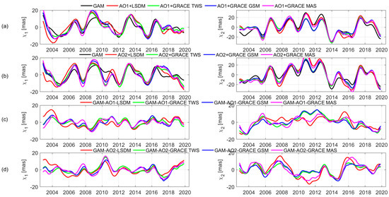
Figure 5.
Comparison between observed geodetic excitation functions and (a) monthly geophysical excitations for AO1 improved by HAM LSDM hydrological model, GRACE GSM, GRACE TWS, and GRACE MAS gravimetric excitations; (b) monthly geophysical excitations for AO2 improved by HAM LSDM hydrological model, GRACE GSM, GRACE TWS, and GRACE MAS gravimetric excitations; (c) differences between GAM and the sum of AO1 + HAM; and (d) differences between GAM and the sum of AO2 + HAM, for and equatorial components.
Table 2.
RMS of the geodetic and geophysical interannual PM excitations improved by different HAM excitations.
In order to show the changes between the observed GAM excitations and the geophysical ones, time series of the differences between GAM and the sum of AO1 + HAM and AO2 + HAM were plotted and are shown in Figure 5c,d, with their RMS values displayed in Table 3. From these results it may be found that atmospheric, ocean, and land hydrology geophysical models do not jointly represent the total original interannual geodetic excitations. The RMS value of the component is reduced to mas for the time series, and to mas for the time series for the component. This may be caused by the fact that current global water storage models generally suffer from limitations, such as groundwater storage omissions or inadequately modelled contributions from the ice caps. A further problem, which affects the compatibility between interannual PM and geophysical excitations, is the appropriate treatment of mass conservation contained in the atmosphere, ocean, and inland freshwater models.
Table 3.
RMS of the differences between geodetic and geophysical interannual PM excitations improved by different HAM excitations.
Additionally, the rates of variance explained and the correlation coefficients between geodetic GAM and geophysical excitations improved by the HAM excitations are computed and presented in Figure 6. The improved correlation between geodetic time series and geophysical ones is due to the component of PM. The AO2 + GRACE TWS time series correlate with the GAM excitations to a level of , and explain the GAM interannual oscillations in . For the component, other geophysical excitations computed for the AO2 combination better explain GAM excitations than the AO1 combination. In the case of the component, the improved completeness is between GAM and AO1 + GRACE GSM, AO1 + GRACE TWS, and AO1 + GRACE MAS. However, the rates of variance explained reached the highest value of for the AO1 + TWS combination, and the correlation coefficient was found to be the best for AO1 + GARCE MAS excitation at .
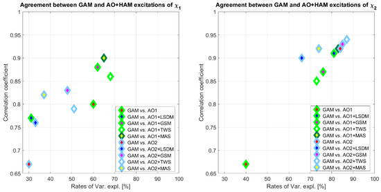
Figure 6.
Correlation coefficients and variance explained rates between geodetic and geophysical interannual PM excitations improved by different HAM excitations, for (left panel), and (right panel).
To understand and quantify interannual oscillations for the observed GAM and geophysical excitations, a linear trend was removed from all the time series using unweighted least squares, and then Fourier spectral analyses (FTBPF Fourier Transform Band Pass Filter, [55]) were performed to identify dominant periods of variation. The spectra of the complex-valued components of for the GAM and geophysical excitations AO1 and AO2, improved by HAM excitations, are shown in Figure 7a–c. These spectra were computed using Fourier Transform Band Pass Filters (FTBPF; [55]) with a 50- and 4500-day cutoff.
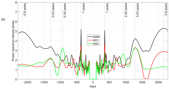
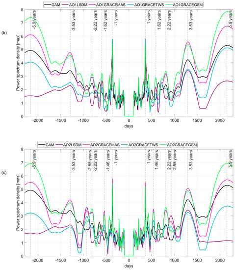
Figure 7.
(a) Fourier Transform Band Pass Filter (FTBPF) amplitude spectra for the different complex GAM excitations and: (a) AO1 and AO2 geophysical excitations; (b) AO1 geophysical excitations improved by HAM LSDM, GRACE GSM, GRACE TWS, and MAS excitations; and (c) AO2 geophysical excitations improved by HAM LSDM, GRACE GSM, GRACE TWS, and MAS excitation functions.
The spectra of all considered functions show seasonal oscillations, and number of peaks at periods between and years. In this study, the seasonal oscillations were not of interest, but they are shown to compare signal strength. Excluding seasonal oscillations, the largest peak present in GAM and AO1 geophysical models in the prograde direction was at around years, and this peak does not appear in retrograde components, both for AO1 and AO2 (see Figure 7a). Other common peaks in both the prograde and retrograde directions, year oscillations (prominent in prograde part) are in GAM and AO1 and AO2 excitations, wherein the signal of GAM is stronger. The year peak in retrograde oscillations are noted for both AO1 and AO2 geophysical combinations.
Considering the influence of land hydrology on geophysical AO1 and AO2 excitations, a geophysical signal power amplification for AO1 + HAM and AO2 + HAM was generally found. The power of the prograde and retrograde oscillations increased, especially after adding the influence of gravimetric excitation functions from GRACE data (Figure 7b,c). However, when using the HAM LSDM hydrological model for this purpose, the -year peak did not appear. For the GRACE GSM and GRACE MAS excitation functions, the signal for the - and -year oscillations was overestimated in contrast to geodetic observed GAM excitations, both in the prograde and retrograde components.
Both the prograde and retrograde spectra of geophysical excitations reveal other peaks from - to -year oscillations although less prominent than in geodetic GAM excitations.
4. Discussion
In this study, different combinations of geophysical models were analyzed to estimate the total effect of atmospheric and oceanic excitations on PM compared to GAM excitations, considering complex-valued components (). The first combination, AO1, is a combined model of atmospheric NCEP/NCAR AAM and oceanic ECCO kf080 OAM models. The second combination, AO2, associates the ECMWF AAM model with the MPIOM OAM one. For each model, their mass and motion, in terms of AAM and OAM, were compared with GAM excitations at interannual time scales. It was found that all mass and motion terms from different AAM and OAM models play an important role at interannual PM and none of them may be considered negligible. In addition, the mass terms for both AAM models, NCEP/NCAR and ECMWF, show high correlations between each other. However, some important differences between motion terms for different AAM models were found, which were also found in previous studies [56,57]. Some discrepancies between the ECCO and MPIOM OAM models were also found. However, neither the AO1 nor the AO2 combinations were able to close the “geodetic budget” at interannual time scales. Thus, none of these combinations may be selected as a better representation of geophysical fluid mass changes. It was also shown before that differences in various AAM, and especially OAM models, are pretty large and are the source of not closing the polar motion excitation budget (e.g., [5,10,58]).
The effects of changes in freshwater, in the form of ice, snow, permafrost, lakes, glaciers, groundwater, soil moisture, and vegetation on PM are poorly understood, particularly at interannual periods. Because various forms of Terrestrial Water Storage (TWS), are often omitted in direct measurements, it is difficult to model their global distribution compared to atmospheric or oceanic masses. However, since 2002, the GRACE satellite has been providing data sources for investigating inland freshwater at a global scale. Thus, the potential of different solutions calculated from GRACE data to study the interannual impact of land hydrology to PM was also investigated. To achieve this, the latest Release-06 data from CSR in the form of GSM, TWS, and mascon (MAS) solutions to compute hydrological excitations were used. Additionally, HAM from the LSDM hydrological model was used too. It should be kept in mind that long-term trends (decadal oscillations), presumably due to the melting of ice in Greenland and Antarctica, core-mantle coupling effects and others, and interannual variations, are not captured for MPIOM ocean and LSDM hydrological models [59]. Model-based interannual variations present in AAM ECMWF are reliable as they lead to long-periodic signals due to long-term water mass redistribution. However, changes in the ECMWF background models cause artificial jumps in the overall HAM LSDM variations [59]. The effects of different HAM solutions on GAM excitations were also considered by adding this effect to both the AO1 and AO2 geophysical excitations studied.
All comparisons were found to have a better result for the component than for the . This may be due to the fact that atmospheric and oceanic contributions to are more reliably modelled than values. The higher quality of modelled AAM effects on can be explained by the fact that atmospheric mass changes can be more accurately modelled for , rather than for . This is related to a generally higher sensitivity of to mass changes over land as compared to , as a result of the particular land/ocean distributions on the Earth (e.g., [10,27]).
After the decomposition of the complex-valued geodetic and geophysical excitations into prograde and retrograde parts, the power spectra obtained by the FTBPF method revealed oscillations with periods of around , , and years for the prograde and retrograde geodetic and geophysical terms. The strongest oscillations for a period of years was achieved by improving both AO1 and AO2 geophysical oscillations with HAM computed from GRACE GSM and MAS solutions. Similarly, the GRACE GSM and GRACE MAS hydrological excitation functions improved both AO1 and AO2 geophysical excitations both in prograde and retrograde directions to improve the year period oscillations. Previous studies have also noticed to year oscillations in observed PM excitations [12,60].
The analysis presented in this study may be affected by a number of error sources. While PM is one of the most accurately determined geodetic quantities, errors are present in model-based AAM, OAM, and HAM excitations. Inadequate modeling of atmospheric and oceanic effects is the main source of hydrological excitations, since during GRACE data processing, modelled AAM and OAM contributions are removed from the solution during the de-aliasing process. Other important error sources may be the omission of global mass conservation from geophysical fluid layers or model deficiencies like unmodeled processes as well.
5. Conclusions
This paper compares interannual variability in the complex components of different geophysical excitation time series, , reflecting changes in the hydro-atmosphere signal in polar motion with respect to geodetic excitation functions computed from observed polar motion coordinates.
It was found, that the NCEP/NCAR and ECMWF mass components of atmospheric excitations are very similar, both in and components, while their motion parts differ significantly, especially in component. Similarly, some inconsistency between mass and motion terms of ECCO kf080 and MPIOM oceanic models were found.
The geodetic and geophysical AO+HAM excitation models yielded better results when compared with GAM, than those with just the AAM and OAM models. Whereas the AO1 + HAM LSDM and AO2 + HAM LSDM excitations were less correlated with GAM than geophysical excitations, which were improved by different GRACE solutions. Furthermore, all comparisons between GAM and the jointly effect of hydro-atmosphere AO+HAM were found to be in a greater degree for the χ2 than for the χ1 component.
Differences between geodetic GAM excitations and hydro-atmosphere signal of AO+HAM indicated that some unexplained interannual signal remains in residuals time series GAM-AO-HAM.
The oscillations with periods of around , , and years for the prograde and retrograde geodetic and geophysical terms were revealed. Wherein, the GRACE MAS and GSM solutions improved the 5.9- and 3.53-year oscillations both in prograde and retrograde components.
The major conclusion of this study is that the hydro-atmosphere signals in polar motion, studied here as the sum of AAM, OAM, and HAM excitations taken from different models and satellite observations, should be improved in order to achieve better consistency between geodetic GAM and AO+HAM excitation functions, especially in the interannual part of oscillations. A good understanding of geodetic and geophysical angular momentum at different time scales is also essential for improving the modelling of external components of the Earth’s systems, namely, the atmosphere, oceans, hydrosphere, and cryosphere. Additional improvements in AAM, OAM, and HAM excitations, especially coming from GRACE/GRACE-FO data, may contribute to achieving better consistency between GAM and geophysical AO+HAM excitations at interannual time scales.
Funding
This research received no external funding.
Institutional Review Board Statement
Not applicable.
Informed Consent Statement
Not applicable.
Data Availability Statement
The data that support the findings of this study are available in International Earth Rotation and Reference System Service website, and in GRACE Gravity Recovery and Climate Experiment website. These data were derived from the following resources available in the public domain: https://www.iers.org/, http://www2.csr.utexas.edu/grace/, accessed on 1 November 2021.
Acknowledgments
Final version of the paper benefited from the helpful suggestions of the referees. The constructive comments by Piotr Olszewski are gratefully acknowledged.
Conflicts of Interest
The authors declare no conflict of interest.
References
- Chao, B.F. Excitation of Earth’s polar motion by atmospheric angular momentum variations: 1980–1990. Geophys. Res. Lett. 1993, 20, 253–256. [Google Scholar] [CrossRef]
- Ponte, R.; Stammer, D.; Marshall, D. Oceanic signals in observed motions of the Earth’s pole of rotation. Nature 1998, 391, 476–479. [Google Scholar] [CrossRef]
- Shindelegger, M.; Salstein, D.; Böm, J. Recent estimates of Earth-atmosphere interaction torques and their use in studying polar motion variability. J. Geophys. Res. Solid Earth 2013, 118, 4586–4598. [Google Scholar] [CrossRef]
- Dobslaw, H.; Dill, R.; Grötsch, A.; Brzezinski, A.; Thomas, M. Seasonal polar motion excitation from numerical models of atmosphere, ocean, and continental hydrosphere. J. Geophys. Res. Solid Earth 2010, 115, B10406. [Google Scholar] [CrossRef]
- Brzeziński, A.; Nastula, J.; Kołaczek, B. Seasonal excitation of polar motion estimated from recent geophysical models and observations. J. Geodyn. 2009, 48, 235–240. [Google Scholar] [CrossRef]
- Bizouard, C. Geophysical Modelling of the Polar Motion; De Gruyter: Berlin, Germany; Boston, MA, USA, 2020. [Google Scholar] [CrossRef]
- Doubrovine, P.V.; Steinberger, B.; Torsvik, T. Absolute plate motions in a reference frame defined by moving hotspots in the Pacific, Atlantic and Indian Oceans. J. Geophys. Res. 2012, 117, B09101. [Google Scholar] [CrossRef]
- Mitrovica, J.X.; Wahr, J. Ice age Earth rotation. Annu. Rev. Earth Planet. Sci. 2011, 39, 577–616. [Google Scholar] [CrossRef]
- Śliwińska, J.; Nastula, J.; Dobslaw, H.; Dill, R. Evaluating Gravimetric Polar Motion Excitation Estimates from the RL06 GRACE Monthly-Mean Gravity Field Models. Remote Sens. 2020, 12, 930. [Google Scholar] [CrossRef]
- Meyrath, T.; van Dam, T. A comparison of interannual hydrological polar motion excitation from GRACE and geodetic observations. J. Geodyn. 2016, 99, 1–9. [Google Scholar] [CrossRef]
- Chen, J.L.; Wilson, C.R.; Ries, J.C.; Tapley, B.D. Rapid ice melting drives Earth’s pole to the east. Geophys. Res. Lett. 2013, 40, 2625–2630. [Google Scholar] [CrossRef]
- Chen, J.; Wilson, C.R.; Kuang, W.; Chao, B.F. Interannual Oscillations in Earth Rotation. J. Geophys. Res. Solid Earth 2019, 124, 13404–13414. [Google Scholar] [CrossRef]
- Abdi, H.; Williams, L.J. Principal component analysis. Wiley Interdiscip. Rev. Comput. Stat. 2010, 2, 433–459. [Google Scholar] [CrossRef]
- Ghil, M.; Allen, M.R.; Dettinger, M.D.; Ide, K.; Kondrashov, D.; Mann, M.E.; Robertson, A.W.; Saunders, A.; Tian, Y.; Varadi, F.; et al. Advanced spectral methods for climatic time series. Rev. Geophys. 2002, 40, 3-1–3-41. [Google Scholar] [CrossRef]
- Luzano, W.I. Multivariate Extension of the Singular Spectrum Analysis A New Tool in Understanding the Intraseasonal-Oscillation (ISO) of Philippines Summer Monsoon and its Association with Extreme Rainfall Events. Glob. NEST J. 2020, 22, 400–407. [Google Scholar] [CrossRef]
- Oropeza, V.; Sacchi, M. Simultaneous seismic data denoising and reconstruction via multichannel singular spectrum analysis. Geophysics 2011, 76, V25–V32. [Google Scholar] [CrossRef]
- Vautard, R.; You, P.; Ghil, M. Singular-spectrum analysis: A toolkit for short, noisy chaotic signals. Phys. D Nonlinear Phenom. 1992, 58, 95–126. [Google Scholar] [CrossRef]
- Jin, X.; Liu, X.; Guo, J.; Shen, Y. Analysis and prediction of polar motion using MSSA method. Earth Planets Space 2021, 73, 147. [Google Scholar] [CrossRef]
- Jin, X.; Liu, X.; Guo, J.; Shen, Y. Multi-Channel Singular Spectrum Analysis on Geocenter Motion and Its Precise Prediction. Sensors 2021, 21, 1403. [Google Scholar] [CrossRef]
- Broomhead, D.; King, G. Nonlinear Phenomena and Chaos; Sarkar, S., Ed.; Adam Hilger Ltd.: Bristol, UK; Boston, MA, USA, 1986; pp. 113–144. [Google Scholar]
- Broomhead, D.S.; King, G.P. Extracting qualitative dynamics from experimental data. Phys. D Nonlinear Phenom. 1986, 20, 217–236. [Google Scholar] [CrossRef]
- Vautard, R.; Ghil, M. Singular spectrum analysis in nonlinear dynamics, with applications to paleoclimatic time series. Phys. D Nonlinear Phenom. 1989, 35, 395–424. [Google Scholar] [CrossRef]
- Bizouard, C.; Gambis, D. The Combined Solution C04 for Earth Orientation Parameters Consistent with International Terrestrial Reference Frame 2005. In Geodetic Reference Frames; Drewes, H., Ed.; Springer: Berlin/Heidelberg, Germany, 2009; Volume 134, pp. 265–270. [Google Scholar] [CrossRef]
- Gros, R. 3.09—Earth Rotation Variations—Long Period. Treatise Geophys. 2007, 3, 239–294. [Google Scholar] [CrossRef]
- Barnes, R.T.H.; Hide, R.; White, A.A.; Wilson, C.A. Atmospheric Angular Momentum Fluctuations, Length-of-Day Changes and Polar Motion. Proc. R. Soc. Lond. 1983, 387, 31–73. [Google Scholar] [CrossRef]
- Dickman, S.R. Evaluation of “effective angular momentum function” formulations with respect to core-mantle coupling. J. Geophys. Res. Solid Earth 2003, 108. [Google Scholar] [CrossRef]
- Eubanks, M. Variations in the Orientation of the Earth. In Contributions of Space Geodesy to Geodynamics; Smith, D.E., Turcotte, D.L., Eds.; American Geophysical Union: Washington, DC, USA, 1993. [Google Scholar]
- Lambeck, K. The Earth’s Variable Rotation: GeophysicalCauses and Consequences; Cambridge University Press: New York, NY, USA, 1980. [Google Scholar] [CrossRef]
- Gross, R. Theory of Earth Rotation Variations. In Proceedings of the VIII Hotine-Marussi Symposium on Mathematical Geodesy, Rome, Italy, 17–21 June 2013. [Google Scholar] [CrossRef]
- Göttl, F.; Schmidt, M.; Seitz, F. Mass related excitation of polar motion: An assessment of the new RL06 GRACE gravity field models. Earth Planets Space 2018, 70, 195. [Google Scholar] [CrossRef]
- Ray, J.; Rebischung, P.; Griffiths, J. IGS polar motion measurement accuracy. Geod. Geodyn. 2017, 8, 413–420. [Google Scholar] [CrossRef]
- Kalnay, E.; Kanamitsu, M.; Zhu, Y.; Chelliah, M.; Ebisuzaki, W.; Higgins, W.; Janowiak, J.; Mo, K.C.; Ropelewski, C.; Wang, J.; et al. The NCEP/NCAR 40-Year Reanalysis Project. Bull. Am. Meteorol. Soc. 1996, 77, 437–472. [Google Scholar] [CrossRef]
- Salstein, D.A.; Kann, D.M.; Miller, A.J.; Rosen, R.D. The Sub-bureau for Atmospheric Angular Momentum of the International Earth Rotation Service: A Meteorological Data Center with Geodetic Applications. Bull. Am. Meteorol. Soc. 1993, 74, 67–80. [Google Scholar] [CrossRef]
- Zhou, Y.H.; Salstein, D.A.; Chen, J.L. Revised atmospheric excitation function series related to Earth’s variable rotation under consideration of surface topography. J. Geophys. Res. Atmos. 2006, 111, D12108. [Google Scholar] [CrossRef]
- Jin, S.; Chambers, D.P.; Tapley, B.D. Hydrological and oceanic effects on polar motion from GRACE and models. J. Geophys. Res. Solid Earth 2010, 115, B02403. [Google Scholar] [CrossRef]
- Fukumori, I.; Raghunath, R.; Fu, L.L.; Chao, Y. Assimilation of TOPEX/Poseidon altimeter data into a global ocean circulation model: How good are the results? J. Geophys. Res. 1999, 25, 25647–25665. [Google Scholar] [CrossRef]
- Fukumori, I.; Lee, T.; Menemenlis, D.; Fu, L.-L.; Cheng, B.; Tang, B.; Xing, Z.; Giering, R. A dual assimilation system for satellite altimetry. In Proceedings of the Joint TOPEX/Poseidon and Jason—1 Science Working Team Meeting, Miami, FL, USA, 15–17 November 2000. [Google Scholar]
- Gross, R.S.; Fukumori, I.; Menemenlis, D. Atmospheric and oceanic excitation of the Earth’s wobbles during 1980–2000. J. Geophys. Res. 2003, 108. [Google Scholar] [CrossRef]
- Dobslaw, H.; Dill, R. Predicting Earth orientation changes from global forecasts of atmosphere-hydrosphere dynamics. Adv. Space Res. 2018, 4, 1047–1054. [Google Scholar] [CrossRef]
- Yu, N.; Ray, J.; Li, J.; Chen, G.; Chao, N.; Chen, W. Intraseasonal variations in atmospheric and oceanic excitation of length-of-day. Earth Space Sci. 2021, 8, e2020EA001563. [Google Scholar] [CrossRef]
- Dill, R.; Dobslaw, H. Seasonal Variations in Global Mean Sea-Level and Consequences on the Excitation of Length-of-Day Changes. Geophys. J. Int. 2019, 218, 801–816. [Google Scholar] [CrossRef]
- Jungclaus, J.H.; Fischer, N.; Haak, H.; Lohmann, K.; Marotzke, J.; Matei, D.; Mikolajewicz, U.; Notz, D.; Storch, J.S. Characteristics of the ocean simulations in the Max Planck Institute Ocean Model (MPIOM) the ocean component of the MPI-Earth system model. J. Adv. Modelin Earth Syst. 2013, 2, 422–446. [Google Scholar] [CrossRef]
- Hagemann, S.; Gates, L.D. Validation of the hydrological cycle of ECMWF and NCEP reanalyses using the MPI hydrological discharge model. J. Geophys. Res. 2001, 106, 1503–1510. [Google Scholar] [CrossRef]
- Hagemann, S.; Gates, L.D. Improving a subgrid runoff parameterization scheme for climate models by the use of high resolution data derived from satellite observations. Clim. Dyn. 2003, 21, 349–359. [Google Scholar] [CrossRef]
- Chen, J.L.; Wilson, C.R. Low degree gravity changes from GRACE, earth rotation, geophysical models and satellite laser ranging. J. Geophys. Res. Solid Earth 2008, 113, B06205. [Google Scholar] [CrossRef]
- Dobslaw, H.; Wolf, I.; Dill, R.; Poropat, L.; Thomas, M.; Dahle, C.; Esselborn, S.; Konig, R.; Flechtner, R. A new high-resolution model of non–tidal atmosphere and ocean mass variability for de-aliasing of satellite gravity observations: AOD1B RL06. Geophys. J. Int. 2017, 211, 263–269. [Google Scholar] [CrossRef]
- Śliwińska, J.; Wińska, M.; Nastula, J. Preliminary Estimation and Validation of Polar Motion Excitation from Different Types of the GRACE and GRACE Follow-On Missions Data. Remote Sens. 2020, 12, 3490. [Google Scholar] [CrossRef]
- Golyandina, N.; Korobeynikov, A. Basic Singular Spectrum Analysis and forecasting with R. Comput. Stat. Data Anal. 2014, 71, 934–954. [Google Scholar] [CrossRef]
- Growth, A.; Ghil, M. Monte Carlo Singular Spectrum Analysis (SSA) Revisited: Detecting Oscillator Clusters in Multivariate Datasets. J. Clim. 2015, 28, 7873–7893. [Google Scholar] [CrossRef]
- Golyandina, N.; Stepanov, D. SSA-Based approaches to analysis and forecast of multidimentional time series. In Proceedings of the 5th St. Petersburg Workshop on Simulation, Saint Petersburg, Russia, 26 June–2 July 2005. [Google Scholar]
- Plaut, G.; Vautard, R. Spells of low-frequency oscillations and weather regimes in the northern hemisphere. J. Atmos. Sci. 1994, 51, 210–236. [Google Scholar] [CrossRef]
- Winska, M.; Nastula, J.; Salstein, D. Hydrological excitation of polar motion by different variables from the GLDAS models. J. Geod. 2017, 91, 1461–1473. [Google Scholar] [CrossRef]
- Chen, J.L.; Wilson, C.R.; Chao, B.F.; Shum, C.K. Hydrological and oceanic excitations to polar motion andlength-of-day variation. Geophys. J. Int. 2000, 141, 149–156. [Google Scholar] [CrossRef]
- Seoane, L.; Nastula, J.; Bizouard, C.; Gambis, D. Hydrological Excitation of Polar Motion Derived from GRACE Gravity Field Solutions. Int. J. Geophys. 2011, 2011, 174396. [Google Scholar] [CrossRef]
- Kosek, W. Time variable band pass filter spectra of real and complex-valued polar motion series. Artif. Satell. Planet. Geod. 1995, 30, 27–43. [Google Scholar]
- Aoyama, Y.; Naito, I. Wind contributions to the Earth’s angular momentum budgets in seasonal variation. J. Geophys. Res. 2000, 105, 12417–12431. [Google Scholar] [CrossRef]
- Masaki, Y. Wind field differences between three meteorological reanalysis data sets detected by evaluating atmospheric excitation of Earth rotation. J. Geophys. Res. 2008, 113. [Google Scholar] [CrossRef]
- Wińska, M.; Ślwiwińska, J. Assessing hydrological signal in polar motion from observations and geophysical models. Studia Geophys. Et Geod. 2019, 63, 95–117. [Google Scholar] [CrossRef]
- Dobslaw, H.; Dill, R.E. Effective Angular Momentum Functions from Earth System Modelling at GeoForschungsZentrum in Potsdam; Technical Report; Revision 1.1 (18 March 2019); GFZ: Potsdam, Germany, 2019; Available online: http://rz-vm115.gfz-potsdam.de:8080/repository (accessed on 24 December 2019).
- Abarca del Rio, R.; Cazenave, A. Interannual variations in the Earth’s polar motion for 1963–1991: Comparison with atmospheric angular momentum over 1980–1991. Geophys. Res. Lett. 1994, 21, 2361–2364. [Google Scholar] [CrossRef]


Publisher’s Note: MDPI stays neutral with regard to jurisdictional claims in published maps and institutional affiliations. |
© 2021 by the author. Licensee MDPI, Basel, Switzerland. This article is an open access article distributed under the terms and conditions of the Creative Commons Attribution (CC BY) license (https://creativecommons.org/licenses/by/4.0/).