
Evaluation of the Integrity Risk for Precise Point Positioning


Abstract
1. Introduction
2. Methods
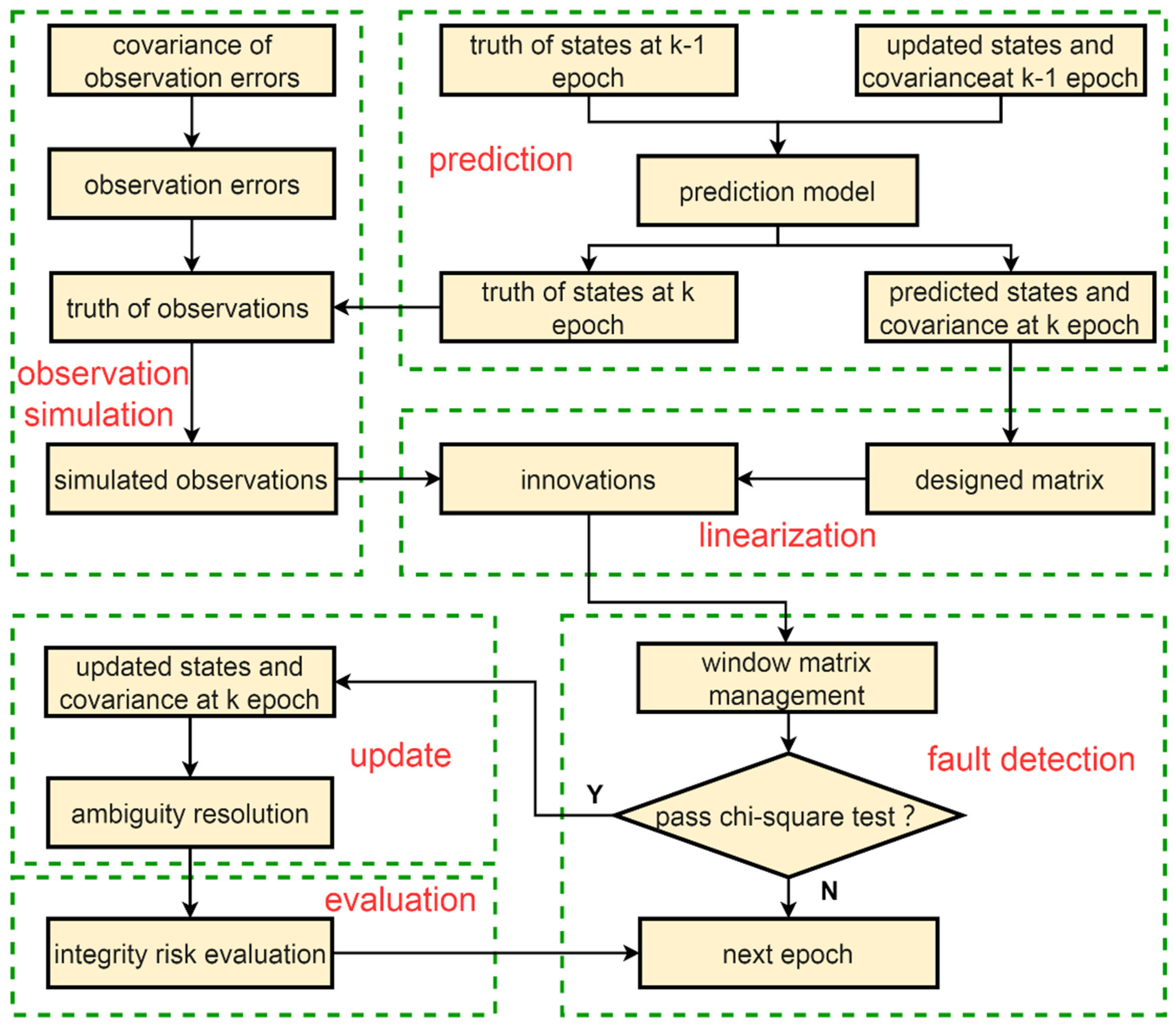
2.1. EKF Processing
2.2. Integrity Risk Evaluation
2.2.1. The Distribution of PE and Detector
2.2.2. Fault Mode
2.2.3. The Worst-Case Integrity Risk
3. Experiments
3.1. Design of the Simulated PPP
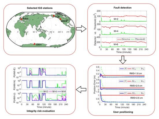
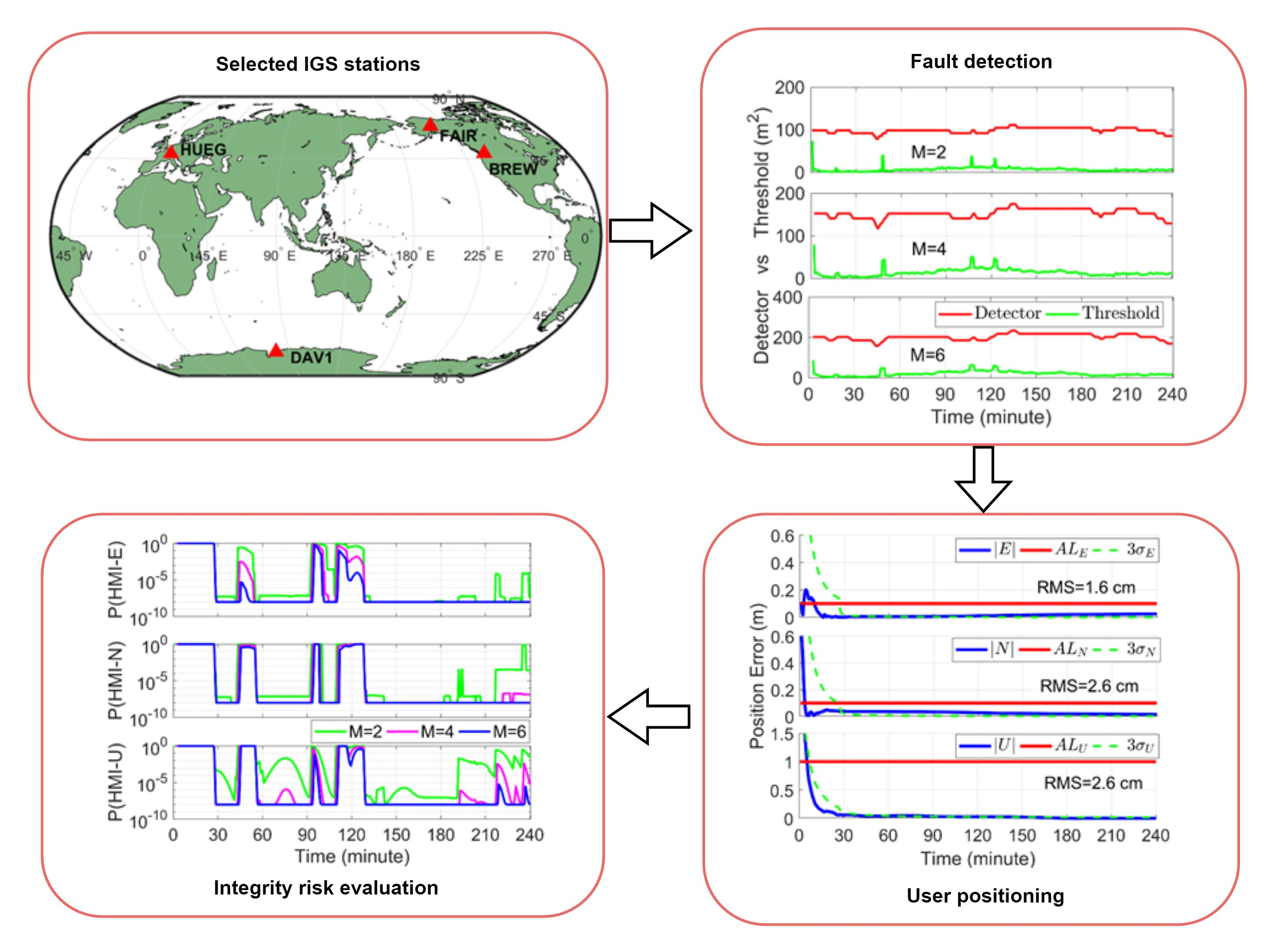
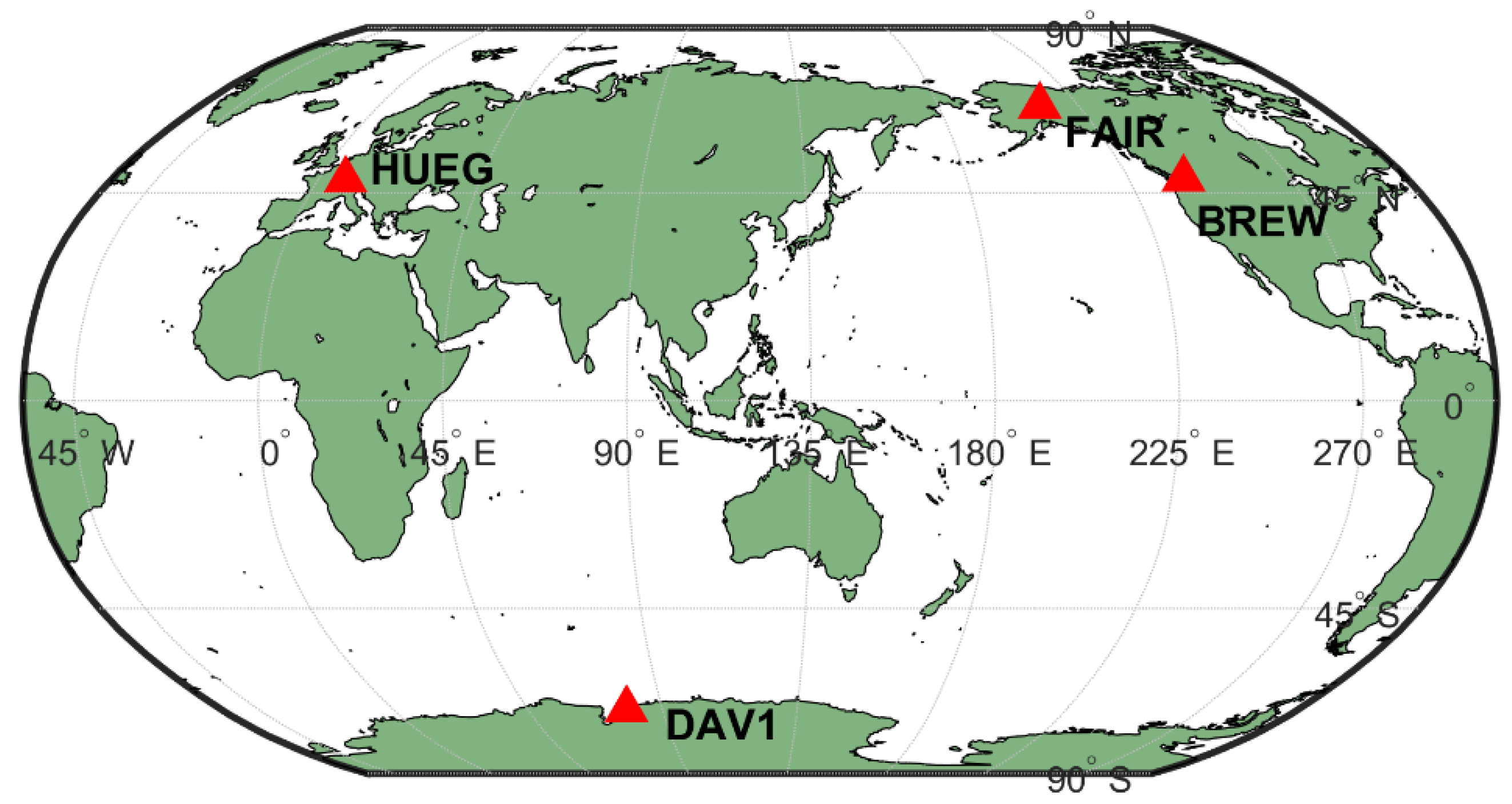
3.2. Experimental PPP Test
4. Results and Discussion
4.1. Simulated Results
4.2. Experimental Results
5. Conclusions
Author Contributions
Funding
Institutional Review Board Statement
Informed Consent Statement
Data Availability Statement
Acknowledgments
Conflicts of Interest
Appendix A
Appendix B
References
- Kouba, J.; Héroux, P. Precise Point Positioning Using IGS Orbit and Clock Products. GPS Solut. 2001, 5, 12–28. [Google Scholar] [CrossRef]
- An, X.; Meng, X.; Jiang, W. Multi-constellation GNSS precise point positioning with multi-frequency raw observations and dual-frequency observations of ionospheric-free linear combination. Satell. Navig. 2020, 1, 7. [Google Scholar] [CrossRef]
- Jin, S.; Su, K. PPP models and performances from single- to quad-frequency BDS observations. Satell. Navig. 2020, 1, 16. [Google Scholar] [CrossRef]
- Choy, S.; Bisnath, S.; Rizos, C. Uncovering common misconceptions in GNSS Precise Point Positioning and its future prospect. GPS Solut. 2017, 21, 13–22. [Google Scholar] [CrossRef]
- Ge, M.; Gendt, G.; Rothacher, M.; Shi, C.; Liu, J. Resolution of GPS carrier-phase ambiguities in Precise Point Positioning (PPP) with daily observations. J. Geod. 2008, 82, 389–399. [Google Scholar] [CrossRef]
- Liu, S.; Yuan, Y. A Method to Accelerate the Convergence of Satellite Clock Offset Estimation Considering the Time-Varying Code Biases. Remote Sens. 2021, 13, 2714. [Google Scholar] [CrossRef]
- Liu, T.; Yuan, Y.; Zhang, B.; Wang, N.; Tan, B.; Chen, Y. Multi-GNSS precise point positioning (MGPPP) using raw observations. J. Geod. 2017, 91, 253–268. [Google Scholar] [CrossRef]
- Geng, J.; Guo, J.; Meng, X.; Gao, K. Speeding up PPP ambiguity resolution using triple-frequency GPS/BeiDou/Galileo/QZSS data. J. Geod. 2020, 94, 6. [Google Scholar] [CrossRef]
- Chen, Y.; Gao, W.; Chen, X.; Liu, T.; Liu, C.; Su, C.; Lu, J.; Wang, W.; Mu, S. Advances of SBAS authentication technologies. Satell. Navig. 2021, 2, 12. [Google Scholar] [CrossRef]
- Heßelbarth, A.; Wanninger, L. SBAS orbit and satellite clock corrections for precise point positioning. GPS Solut. 2013, 17, 465–473. [Google Scholar] [CrossRef]
- Zhang, B.; Chen, Y.; Yuan, Y. PPP-RTK based on undifferenced and uncombined observations: Theoretical and practical aspects. J. Geod. 2019, 93, 1011–1024. [Google Scholar] [CrossRef]
- Geng, J.; Teferle, F.N.; Meng, X.; Dodson, A.H. Towards PPP-RTK: Ambiguity resolution in real-time precise point positioning. Adv. Space Res. 2011, 47, 1664–1673. [Google Scholar] [CrossRef]
- Li, X.; Li, X.; Huang, J.; Shen, Z.; Wang, B.; Yuan, Y.; Zhang, K. Improving PPP–RTK in urban environment by tightly coupled integration of GNSS and INS. J. Geod. 2021, 95, 132. [Google Scholar] [CrossRef]
- Khodabandeh, A. Single-station PPP-RTK: Correction latency and ambiguity resolution performance. J. Geod. 2021, 95, 42. [Google Scholar] [CrossRef]
- De Groot, L.; Infante, E.; Jokinen, A.; Kruger, B.; Norman, L. Precise Positioning for Automotive with Mass Market GNSS Chipsets. In Proceedings of the 31st International Technical Meeting of the Satellite Division of the Institute of Navigation, Miami, FL, USA, 24–28 September 2018; pp. 596–610. [Google Scholar]
- Murrian, M.; Gonzalez, C.W.; Humphreys, T.E.; Pesyna, K.M.; Shepard, D.P.; Kerns, A.J. Low-cost precise positioning for automated vehicles. GPS World 2016, 27, 32–39. [Google Scholar]
- Alkan, R.M.; Saka, M.H.; Ozulu, İ.M.; İlçi, V. Kinematic precise point positioning using GPS and GLONASS measurements in marine environments. Measurement 2017, 109, 36–43. [Google Scholar] [CrossRef]
- Yang, Y.; Mao, Y.; Sun, B. Basic performance and future developments of BeiDou global navigation satellite system. Satell. Navig. 2020, 1, 1–8. [Google Scholar] [CrossRef]
- Zhu, N.; Marais, J.; Betaille, D.; Berbineau, M. GNSS Position Integrity in Urban Environments: A Review of Literature. IEEE Trans. Intell. Transp. Syst. 2018, 19, 2762–2778. [Google Scholar] [CrossRef]
- Norman, L.; Infante, E.; De Groot, L. Integrity performance for precise positioning in automotive. In Proceedings of the 32nd International Technical Meeting of the Satellite Division of the Institute of Navigation, Miami, FL, USA, 16–20 September 2019; pp. 1653–1663. [Google Scholar]
- Du, Y.; Wang, J.; Rizos, C.; El-Mowafy, A. Vulnerabilities and integrity of precise point positioning for intelligent transport systems: Overview and analysis. Satell. Navig. 2021, 2, 3. [Google Scholar] [CrossRef]
- El-Mowafy, A. On detection of observation faults in the observation and position domains for positioning of intelligent transport systems. J. Geod. 2019, 93, 2109–2122. [Google Scholar] [CrossRef]
- Li, B.; Qin, Y.; Liu, T. Geometry-based cycle slip and data gap repair for multi-GNSS and multi-frequency observations. J. Geod. 2019, 93, 399–417. [Google Scholar] [CrossRef]
- Ochieng, W.Y.; Sauer, K.; Walsh, D.; Brodin, G.; Griffin, S.; Denney, M. GPS Integrity and Potential Impact on Aviation Safety. J. Navig. 2003, 56, 51–65. [Google Scholar] [CrossRef]
- Pullen, S.; Joerger, M. GNSS Integrity and Receiver Autonomous Integrity Monitoring (RAIM). In Position, Navigation, and Timing Technologies in the 21st Century; Wiley: Piscataway, NJ, USA, 2020; pp. 591–617. [Google Scholar]
- Zabalegui, P.; De Miguel, G.; Perez, A.; Mendizabal, J.; Goya, J.; Adin, I. A Review of the Evolution of the Integrity Methods Applied in GNSS. IEEE Access 2020, 8, 45813–45824. [Google Scholar] [CrossRef]
- Parkinson, B.; Axelrad, P. Autonomous GPS Integrity Monitoring Using the Pseudorange Residual. Navigation 1988, 35, 255–274. [Google Scholar] [CrossRef]
- Walter, T.; Enge, P. Weighted RAIM for Precision Approach. In Proceedings of the 8th International Technical Meeting of the Satellite Division of the Institute of Navigation, Palm Springs, CA, USA, 12–15 September 1996; pp. 1995–2004. [Google Scholar]
- Blanch, J.; Walker, T.; Enge, P.; Lee, Y.; Pervan, B.; Rippl, M.; Spletter, A.; Kropp, V. Baseline advanced RAIM user algorithm and possible improvements. IEEE Trans. Aerosp. Electron. Syst. 2015, 51, 713–732. [Google Scholar] [CrossRef]
- Blanch, J.; Walter, T.; Enge, P.; Lee, Y.; Pervan, B.; Rippl, M.; Spletter, A. Advaced RAIM User Algorithm Description: Integrity Support Message Processing, Fault Detection, Exclusion, and Protection Level Calculation. In Proceedings of the 25th International Technical Meeting of the Satellite Division of the Institute of Navigation, Nashville, TN, USA, 17–21 September 2012; pp. 2828–2849. [Google Scholar]
- Joerger, M.; Pervan, B. Kalman Filter Residual-Based Integrity Monitoring against Measurement Faults. In Proceedings of the AIAA Guidance, Navigation, and Control Conference, Minneapolis, MN, USA, 13–16 August 2012. [Google Scholar]
- Joerger, M.; Pervan, B. Integrity risk of Kalman filter-based RAIM. In Proceedings of the 24th International Technical Meeting of the Satellite Division of the Institute of Navigation, Portland, OR, USA, 19–23 September 2011; pp. 3856–3867. [Google Scholar]
- Tanil, C. Detecting GNSS Spoofing Attacks Using INS Coupling. Ph.D. Thesis, Illinois Institute of Technology, Chicago, IL, USA, December 2016. [Google Scholar]
- Tanil, C.; Khanafseh, S.; Joerger, M.; Pervan, B. Sequential Integrity Monitoring for Kalman Filter Innovations-based Detectors. In Proceedings of the 31st International Technical Meeting of the Satellite Division of the Institute of Navigation, Miami, FL, USA, 24–28 September 2018; pp. 2440–2455. [Google Scholar]
- Arana, G.D.; Hafez, O.A.; Joerger, M.; Spenko, M. Recursive Integrity Monitoring for Mobile Robot Localization Safety. In Proceedings of the 2019 International Conference on Robotics and Automation, Montreal, QC, Canada, 20–24 May 2019; pp. 305–311. [Google Scholar]
- Feng, S.; Jokinen, A.; Ochieng, W. Integrity Monitoring for Precise Point Positioning. In Proceedings of the the 27th International Technical Meeting of The Satellite Division of the Institute of Navigation, Tampa, FL, USA, 8–12 September 2014; pp. 986–1007. [Google Scholar]
- Jokinen, A.; Feng, S.; Schuster, W.; Ochieng, W.; Hide, C.; Moore, T.; Hill, C. Integrity monitoring of fixed ambiguity Precise Point Positioning (PPP) solutions. Geo-Spat. Inf. Sci. 2013, 16, 141–148. [Google Scholar] [CrossRef]
- Gunning, K.; Blanch, J.; Walter, T.; Groot, L.; Norman, L. Design and evaluation of integrity algorithms for PPP in kinematic applications. In Proceedings of the 31st International Technical Meeting of the Satellite Division of the Institute of Navigation, Miami, FL, USA, 24–28 September 2018; pp. 1910–1939. [Google Scholar]
- Blanch, J.; Gunning, K.; Walter, T.; Groot, L.; Norman, L. Reducing computational load in solution separation for Kalman flters and an application to PPP integrity. In Proceedings of the 32nd International Technical Meeting of the Satellite Division of the Institute of Navigation, Miami, FL, USA, 16–20 September 2019; pp. 720–729. [Google Scholar]
- Blanch, J.; Walter, T.; Norman, L.; Gunning, K.; de Groot, L. Solution Separation-Based FD to Mitigate the Effects of Local Threats on PPP Integrity. In Proceedings of the 2020 IEEE/ION Position, Location and Navigation Symposium, Portland, OR, USA, 20–23 April 2020; pp. 1085–1092. [Google Scholar]
- Madrid, P.F.N.; Fernandez, L.M.; Lopez, M.A.; Samper, M.D.L.; Merino, M.M.R.; Madrid, P.F.N.; Fernndez, L.M.; Lpez, M.A.; Samper, L.; Merino, M.M.R. PPP Integrity for Advanced Applications, Including Field Trials with Galileo, Geodetic and Low-Cost Receivers, and a Preliminary Safety Analysis. In Proceedings of the 29th International Technical Meeting of the Satellite Division of the Institute of Navigation, Portland, OR, USA, 12–16 September 2016; pp. 3332–3354. [Google Scholar]
- Angus, J.E. RAIM with Multiple Faults. Navigation 2006, 53, 249–257. [Google Scholar] [CrossRef]
- Saastamoinen, J. Contributions to the theory of atmospheric refraction. Bulletin Géodésique 1972, 105, 279–298. [Google Scholar] [CrossRef]
- Niell, A.E. Global mapping functions for the atmosphere delay at radio wavelengths. J. Geophys. Res. Solid Earth 1996, 101, 3227–3246. [Google Scholar] [CrossRef]


| Input Information | Settings |
|---|---|
| Navigation system | GPS |
| Calculation interval | 10 (s) |
| Period | 9/19/2021 00:00:00–9/19/2021 02:00:00 |
| Cut-off elevation | 10° |
| Weighted model | Elevation weighted |
| Standard deviation of raw observations | Code: Phase: (cm) |
| Standard deviation of initialized states\process noise | (m) (m) (m) (m) for every epoch (m) (m) |
| 0.1 (m) for the east and north directions and 1 (m) for the up direction | |
| Length of the window | 2 epochs |
| Items | Strategies |
|---|---|
| Navigation system | GPS |
| Frequencies | L1, L2 |
| Calculation interval | 30 (s) |
| Period | 9/19/2021 00:00:00–9/19/2021 04:00:00 |
| Weighted model | Elevation weighted |
| Standard deviation of raw observations | Code: Phase: (cm) |
| Standard deviation of initialized states\process noise | (m) (m) for every epoch (m) (m) |
| Precise satellite orbits and clocks | Products provided by the GFZ center |
| Differential code bias | Corrected by the products provided by the Chinese Academy of Sciences |
| Relativistic effect | Corrected |
| Phase wind-up | Corrected |
| Earth rotation effects and tidal displacements | Corrected by the earth rotation file provided by the GFZ center |
| Antenna phase center offset and variation correction | Corrected by the igs14_2178.atx file |
| Truth of station coordinate | Provided by the igs21P21760.snx file |
| Ambiguity resolution | Fixed and hold mode |
| E | N | U | |
|---|---|---|---|
| 0.3 | 1.0 | 0.8 | 2.5 |
| 0.4 | 1.3 | 1.1 | 3.4 |
| 0.5 | 1.8 | 1.4 | 4.2 |
Publisher’s Note: MDPI stays neutral with regard to jurisdictional claims in published maps and institutional affiliations. |
© 2021 by the authors. Licensee MDPI, Basel, Switzerland. This article is an open access article distributed under the terms and conditions of the Creative Commons Attribution (CC BY) license (https://creativecommons.org/licenses/by/4.0/).
Share and Cite
Xue, B.; Yuan, Y.; Wang, H.; Wang, H. Evaluation of the Integrity Risk for Precise Point Positioning. Remote Sens. 2022, 14, 128. https://doi.org/10.3390/rs14010128
Xue B, Yuan Y, Wang H, Wang H. Evaluation of the Integrity Risk for Precise Point Positioning. Remote Sensing. 2022; 14(1):128. https://doi.org/10.3390/rs14010128
Chicago/Turabian StyleXue, Bing, Yunbin Yuan, Han Wang, and Haitao Wang. 2022. "Evaluation of the Integrity Risk for Precise Point Positioning" Remote Sensing 14, no. 1: 128. https://doi.org/10.3390/rs14010128
APA StyleXue, B., Yuan, Y., Wang, H., & Wang, H. (2022). Evaluation of the Integrity Risk for Precise Point Positioning. Remote Sensing, 14(1), 128. https://doi.org/10.3390/rs14010128