An Object-Based Markov Random Field with Partition-Global Alternately Updated for Semantic Segmentation of High Spatial Resolution Remote Sensing Image

Abstract

The Markov random field (MRF) method is widely used in remote sensing image semantic segmentation because of its excellent spatial (relationship description) ability. However, there are some targets that are relatively small and sparsely distributed in the entire image, which makes it easy to misclassify these pixels into different classes. To solve this problem, this paper proposes an object-based Markov random field method with partition-global alternately updated (OMRF-PGAU). First, four partition images are constructed based on the original image, they overlap with each other and can be reconstructed into the original image; the number of categories and region granularity for these partition images are set. Then, the MRF model is built on the partition images and the original image, their segmentations are alternately updated. The update path adopts a circular path, and the correlation assumption is adopted to establish the connection between the label fields of partition images and the original image. Finally, the relationship between each label field is constantly updated, and the final segmentation result is output after the segmentation has converged. Experiments on texture images and different remote sensing image datasets show that the proposed OMRF-PGAU algorithm has a better segmentation performance than other selected state-of-the-art MRF-based methods.

1. Introduction

Semantic segmentation is an important part of remote sensing image processing, and its goal is to give a special semantic interpretation to the homogeneous regions in the image. The semantic segmentation results of remote sensing images can provide a macro statistical data base for vegetation growth analysis [1], coastline protection [2], urban development [3,4], etc.

Many methods for semantic segmentation have been proposed [5], which can be roughly divided into two categories: supervised and unsupervised. The main difference between the two is whether the classifier requires training samples. The former designs a classifier with undetermined parameters according to specific rules, and obtains a classifier that can identify specific categories by identifying training samples. This category contains many methods, such as: support vector machines (SVMs) [6,7,8], neural network-based algorithms [9,10,11,12,13,14,15], deep learning [16,17,18,19,20,21,22], etc. The latter is based on the image’s own features, directly modeling the image’s data and giving segmentation results, such as: super-pixel [23,24,25,26], Markov random field (MRF) [27,28,29,30,31,32,33,34], conditional random field (CRF) [35,36,37,38,39], level set [40,41,42], etc. Among these methods, MRF is based on the idea of probability statistics, which can consider both image features and spatial information when modeling. It has become a widely used segmentation method, and our research is based on the MRF method.

MRF-based methods usually include two sub-modules [27,31]: the feature field, which describes the image features, and the label field, which describes the spatial relationship between the nodes in the image. The feature field is mainly used to measure the likelihood of the realization of the feature distribution for a given segmentation result for the given image. The label field can calculate the probability of the segmentation realization, presenting the given result based on the defined neighborhood structure. Then, the problem of image semantic segmentation is transformed into, for a given image, how to achieve the realization of maximizing the posterior probability of the label field through the feature field likelihood function and the prior probability of the label field.

The classic MRF [27] method uses pixels as processing units, and updates the segmentation results pixel-by-pixel. After the introduction of wavelet tools, a series of multi-resolution MRF (MRMRF) methods were formed [28,43,44]. This type of method can obtain image features and spatial neighborhood information of different scales on different resolution layers, and the accuracy of the semantic segmentation result is improved. With the development of sensor technology, remote sensing images have shown high spatial resolution development trends, and the returned remote sensing images describe the details of ground objects more clearly. As a result, the sizes of the captured remote sensing images get larger, and the amounts of the calculations for semantic segmentations are significantly increased. Therefore, object-based image analysis (OBIA) [45] was introduced into the MRF, forming object-based MRF (OMRF) [46] for semantic segmentation of remote sensing images. It replaces pixels with small regions, with a certain homogeneity, as the nodes to be processed, which reduces the amount of the calculation and can add some regional features to the feature field modeling. However, the current high spatial resolution remote sensing image requires more pixels to describe a surface target, which makes the spectral value fluctuation range of the same category of the ground object larger. Moreover, the spatial distribution of the same type of feature in the image is not necessarily concentrated, which causes a low accuracy of the segmentation results.

To solve the above problems, many researchers have made efforts based on OMRF. Zheng et al. [28] proposed the multiregion-resolution MRF (MRR-MRF) Model, this method is based on MRMRF and introduces the idea of OBIA. It obtains different granularity region adjacency graphs (RAG) on all resolution layers, and then passes through one-way projection to obtain the original resolution image segmentation results. Yao et al. [44] observed the multi-resolution MRF with the bilateral information (MRMRF-bi) model, which mainly improved the update strategy of MRMRF. This method obtains the RAG at the original resolution and directly projects it to each layer. In the subsequent segmentation update process, each resolution layer is simultaneously affected by the segmentation results of its adjacent upper and lower layers. Zheng et al. [30] proposed the hybrid MRF With multi-granularity information (HMRF-MG), which designs a hybrid label field to integrate and capture the interactions between the pixel-granularity information and the object-granularity information.

The above methods all use the idea of multi-granularity, but at a large-size, high-resolution image pixels belonging to the same category might have sparse spatial distributions and large changes in spectral values. These pixels will have a greater probability of being classified into different categories. In order to solve this problem, simply using multi-granularity does not help much to solve this problem. This paper proposes an object-based Markov random field method with partition-global alternately updated (OMRF-PGAU). First, the given original image is divided into four partition images, with the same size and overlap; then RAGs with different granularity are built on these five images, and OMRF are defined on the RAGs; finally, the original image and the partition images are updated alternately until the segmentation is converged. The alternate update mechanism is, after the original image is self-updated, the segmentation result is projected to each partition image to form a related auxiliary label field, which assists the four partition images to update the segmentation results; after the four partition images are self-updated, their segmentations form the auxiliary label field of the original image, according to the merging mechanism, and affect the update of the original image segmentation result.

The main contributions of the algorithm proposed in this paper can be summarized as follows:

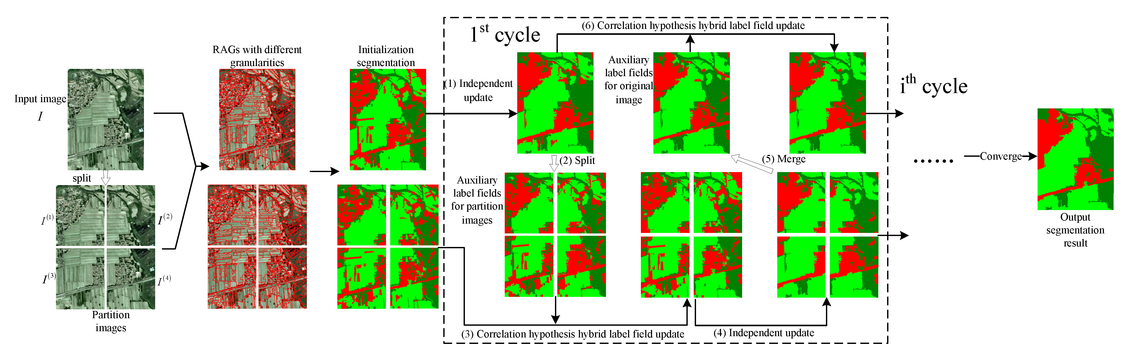
• The original image and the partition images are set so that the segmentation result can be updated alternately, locally and globally. For the original image, in the process of updating the segmentation results, the homogeneity of the region can be considered, and the entire image can be analyzed macroscopically to keep the segmentation results smooth; in the four partition images, the local information can be better explored and the details can be retained. The targets belonging to same category with sparse spatial distribution in the original image is relatively more concentrated in the partitioned image, which is easy to be divided into one class.
• Different granularity is set in the original image and the four partition images. Using different granularities to describe the same target, different area information and spatial information can be obtained, and the inaccuracy due to unreasonable settings of over-segmented regions can be avoided. It can also avoid the update segmentation result falling into the local optimum.
• Correlation assumption of the segmentation results of the original image and the four partition images. For the original image, the auxiliary segmentation label field with an indefinite number of classes obtained by merging the partitioned segmentation results is used; for the partition images, the segmentation result of the original image is projected to each partitioned image to form the auxiliary segmentation label field. Using the correlation assumption, these auxiliary segmentation label layers are combined with the priori segmentation of each image to form a hybrid label field to update the segmentation results for each image.

More details of the proposed OMRF-PGAU has been introduced in the Section 2. The parameter setting of the OMRF-PGAU and the comparative experiments with other methods are presented in Section 3. The discussion of the experimental results are shown in Section 4, and the conclusions of OMRF-PGAU are given in Section 5.

2. Methodology

The OMRF-PGAU method proposed in this paper aims to accelerate the convergence speed of segmentation update and improve the accuracy of segmentation. It uses the idea of alternate updates the segmentation results of original and partitioned images, and constructs the hybrid label field according to the correlation assumption. In this section, the MRF method will be briefly introduced, and then the specific details of the proposed OMRF-PGAU algorithm will be given.

2.1. MRF for Image Segmentation

For a given image I of size $M\times N$, its pixel location index set can be denoted as $S^{pixel}= \left\{\left(m,n\right)\left|1\le m\le M,1\le n\le N\right.\right\}$. Setting the number of categories K, then the segmentation of the image I can be expressed by the following equations.

$$S^{pixel}=\bigcup _{i=1}^K{S}_i$$

(1)

$$S_i\cap S_j=\varnothing ,i\ne j$$

(2)

$$S_i=\left\{\left(m^{\prime },n^{\prime }\right)\left|f\left(m^{\prime },n^{\prime }\right)=s{p}_i\right.\right\}$$

(3)

Equations (1) and (2) indicate that image segmentation is the division of the original image I into K mutually disjoint subsets, and these subsets can be merged into the original image. Equation (3) indicates that the pixels contained in each class are consistent with the specific properties of this class, $s{p}_i$ represents the specific properties of the i-th class.

The MRF method is a graph model method based on probabilistic statistics. It cannot only explore the spectral features of the image, but also the spatial information contained in the image based on the neighborhood relationship.

For the given image I, we can obtain its region adjacency graph (RAG), $G=\left(V,E\right)$. $V=\left\{V_s\left|s\in S\right.\right\}$ is the set of nodes that wait to be segmented. When the node $V_s$ is a pixel, this model is a pixel-based MRF (pMRF). If the $V_s$ represents an over-segmented region which is a set of pixels contained in this region, it’s an object-based MRF (OMRF). Moreover, $E={\left(e_{s,s^{\prime }}\right)}_{∥S∥\times ∥S∥}$ is a 0–1 matrix, which records the adjacency relationship between each node, $e_{s,s^{\prime }}=0$ unless the node s and $s^{\prime }$ are adjacent. The S is the position index set.

Take OMRF as an example, its algorithm flowchart is shown as in Figure 1. Based on the G, two random field can be established: the feature field $Y=\left\{Y_s\left|s\in S\right.\right\}$, and the label field $X=\left\{X_s\left|s\in S\right.\right\}$. $Y_s$ represents the feature vector of the node $V_s$. $X_s$ represents the segmentation label of node $V_s$, which is a random variable valued in the set $\mathsf{\Lambda }=\left\{1,2\cdots ,K\right\}$. K is a preset number of the category. In the case of a given image I, the feature field Y has a unique realization y. Assuming that x is a realization of the label field X, then probability modeling is performed on the feature field; that is, the distribution function of $P\left(Y=y\left|X=x\right.\right)$ is calculated. It means the probability that the feature field is realized as y when the realization of the label field is x. The $P\left(Y=y\left|X=x\right.\right)$ is usually assumed to obey Gaussian mixed model and the features of each node are assumed to be independent of each other. That is,

$$P\left(Y=y\left|X=x\right.\right)=\prod _{s\in S}P\left(Y_s=y_s\left|X_s=x_s\right.\right)$$

(4)

For the label field X, we assume it has Markov property, i.e.,

$$P\left(X_s\left|X_t,t\in S/s\right.\right)=P\left(X_s\left|X_{N_s}\right.\right)$$

(5)

The $N_s$ represents the neighborhood of node $V_s$, $X_{N_s}$ denotes the segmentation labels of the neighborhood nodes of node $V_s$. $V_{s^{\prime }}\in N_s$ when $e_{s,s^{\prime }}=1$. Then the $P\left(X\right)$ can be written as

$$P\left(X\right)=P\left(X_1,X_2,\cdots ,X_{∥S∥}\right)\approx \prod _{s\in S}P\left(X_s\left|X_{N_s}\right.\right)$$

(6)

The $∥S∥$ represents the number of the elements contained in the set S. According to the Hammersley–Clifford theorem [47], the label field X with the neighborhood system $N=\left\{N_s\left|s\in S\right.\right\}$ obeys the Gibbs distribution; that is

$$P\left(X\right)=\frac{1}{Z}·e^{-U\left(X\right)}$$

(7)

where Z is the normalization constant and $U\left(X\right)$ is the potential energy function of all groups contained in the neighborhood of the random field. For each node $V_s$,

$$P\left(X_s=x_s\left|X_{s^{\prime }}=x_{s^{\prime }},V_{s^{\prime }}\in N_s\right.\right)=\frac{e^{-U\left(x_s\right)}}{{\displaystyle \sum _{x_{s^{\prime }}\in \mathsf{\Lambda }}}{e}^{-U\left(x_{s^{\prime }}\right)}}$$

(8)

For the image segmentation problem, it is usually assumed that the potential energy function $U\left(X\right)$ calculates only the energy of the two-point groups, i.e.,

$$U\left(x_s\right)=\sum _{V_{s^{\prime }}\in N_s}{v}_2\left(x_s,x_{s^{\prime }}\right)$$

(9)

$$v_2\left(x_s,x_{s^{\prime }}\right)=\left\{\begin{array}{cc}-\beta & x_s=x_{s^{\prime }}\\ \beta & x_s\ne x_{s^{\prime }}\end{array}\right.$$

(10)

The $\beta$ is potential parameter. By probabilistic modeling of the feature field Y and the label field X, the image segmentation problem can be transformed into: finding the maximized label field posterior probability implementation $\widehat{x}$. That is

$$\begin{array}{cc}\hfill \widehat{x}& =\underset{x}{argmax}P\left(X=x\left|Y=y\right.\right)\hfill \\ \hfill & =\underset{x}{argmax}P\left(Y=y\left|X=x\right.\right)·P\left(X=x\right)\hfill \\ \hfill & =\underset{x}{argmax}\prod _{s\in S}\left[P\left(Y_s=y_s\left|X_s=x_s\right.\right)·P\left(X_s=x_s\right)\right]\hfill \end{array}$$

(11)

2.2. The OMRF-PGAU Model

To solve the problem that the low classification accuracy caused by targets belonging to the same category, but not connected in spatial distribution, and with large differences in spectral values in high-resolution remote sensing images, this paper proposes an object-based Markov random field method with the partition-global alternately updated (OMRF-PGAU) algorithm. Different from the classic MRF method, the OMRF-PGAU algorithm does not always update the segmentation results with the entire image.

The flowchart of OMRF-PGAU is shown in Figure 2.

For a given image I, it is firstly divided into four partition images $I^{\prime }=\left\{I^{\left(1\right)},I^{\left(2\right)},I^{\left(3\right)},I^{\left(4\right)}\right\}$, which have the same size, and there are overlapping areas between every two partition images. Then the RAG, $G=\left(V,E\right)$ for the original image I, and $G^{\prime }=\left\{G^{\left(1\right)},G^{\left(2\right)},G^{\left(3\right)},G^{\left(4\right)}\right\}$, $G^{\left(i\right)}=\left(V^{\left(i\right)},E^{\left(i\right)}\right)$ for the partitioned images $I^{\prime }$ are established, respectively, and the feature field Y, $Y^{\prime }=\left\{Y^{\left(1\right)},Y^{\left(2\right)},Y^{\left(3\right)},Y^{\left(4\right)}\right\}$, and label field X, $X^{\prime }=\left\{X^{\left(1\right)},X^{\left(2\right)},X^{\left(3\right)},X^{\left(4\right)}\right\}$ are formed. The category number for each image is set as $K,K^{\left(1\right)},K^{\left(2\right)},K^{\left(3\right)},K^{\left(4\right)}$ respectively. Finally, the segmentation of the original image and the partition images are alternately updated till the segmentation results are converged.

By constructing two layers, the original image layer and the partition image layer, the global and local semantic information can be considered comprehensively. It enables the segmentation process to mine more image information and effectively reduce the probability of falling into local optimal solutions. The two layers will set different granularity, and the obtained features and spatial relationships will be different accordingly, so that the segmentation process can ensure the smoothness of the region and protect the boundary details of the region at the same time.

Therefore, the image semantic segmentation problem in the classical MRF approach, which can be solved as a single-layer segmentation update problem, needs to be converted into a two-layer joint solution problem in OMRF-PGAU, i.e.,

$$\begin{array}{cc}\hfill \left(\widehat{x},{\widehat{x}}^{\prime }\right)& =\underset{x,x^{\prime }}{argmax}P\left(X=x,X^{\prime }=x^{\prime }\left|Y=y,Y^{\prime }=y^{\prime }\right.\right)\hfill \\ \hfill & =\underset{x,x^{\prime }}{argmax}P\left(Y=y,Y^{\prime }=y^{\prime }\left|X=x,X^{\prime }=x^{\prime }\right.\right)·P\left(X=x,X^{\prime }=x^{\prime }\right)\hfill \end{array}$$

(12)

For the above optimization solution problem, the main difficulty lies in the problem of modeling the likelihood function of the feature field $P\left(Y=y,Y^{\prime }=y^{\prime }\left|X=x,X^{\prime }=x^{\prime }\right.\right)$ and the modeling of the prior partition probability of the label field $P\left(X=x,X^{\prime }=x^{\prime }\right)$. The detailed procedure will be given below.

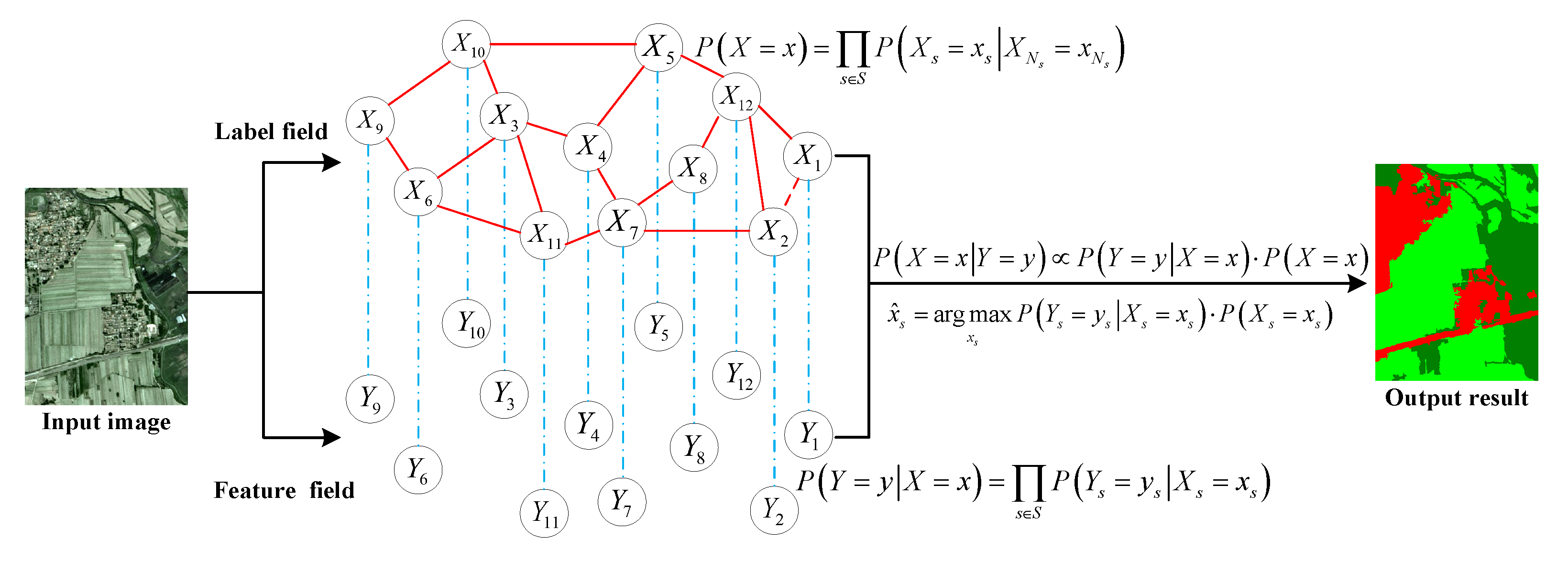
2.2.1. The Probabilistic Modeling of the Feature Field

For the OMRF-PGAU algorithm, it is difficult to directly obtain the feature field likelihood function $P\left(Y=y,Y^{\prime }=y^{\prime }\left|X=x,X^{\prime }=x^{\prime }\right.\right)$. There are many variables in the probability distribution function. So we give some assumptions that are used to assist the derivation to obtain the probability model in a simple form.

In traditional single-layer MRF feature field modeling, it is usually assumed that each node is independent of each other after a given segmentation label; that is, it conforms to Equation (4). In the references [30,32,43], related to multi-layer MRF feature field modeling, they all assume that the features of each layer are independent of each other. Therefore, we put forward the following two hypotheses.

Assumption 1.

For the original image I and partition images$I^{\prime }$, when their priori segmentation results are given, their feature fields are independent of each other. That is

$$\begin{array}{cc}\hfill & P\left(Y=y,Y^{\prime }=y^{\prime }\left|X=x,X^{\prime }=x^{\prime }\right.\right)\hfill \\ \hfill =& P\left(Y=y\left|X=x,X^{\prime }=x^{\prime }\right.\right)·P\left(Y^{\prime }=y^{\prime }\left|X=x,X^{\prime }=x^{\prime }\right.\right)\hfill \\ \hfill =& P\left(Y=y\left|X=x\right.\right)·P\left(Y^{\prime }=y^{\prime }\left|X^{\prime }=x^{\prime }\right.\right)\hfill \\ \hfill =& P\left(Y=y\left|X=x\right.\right)·\prod _{i=1}^{4}P\left(Y^{\left(i\right)}=y^{\left(i\right)}\left|X^{\left(i\right)}=x^{\left(i\right)}\right.\right)\hfill \end{array}$$

(13)

Assumption 2.

The features of the nodes contained in each image are independent of each other nodes, and are only affected by the segmentation results of their own images.

Then Equation (13) can be further written as,

$$\begin{array}{cc}\hfill & P\left(Y=y,Y^{\prime }=y^{\prime }\left|X=x,X^{\prime }=x^{\prime }\right.\right)\hfill \\ \hfill =& \left\{\prod _{s\in S}\left[P\left(Y_s=y_s\left|X_s=x_s\right.\right)\right]\right\}·\prod _{i=1}^4\left\{\prod _{s^{\prime }\in S^i}\left[P\left(Y_{s^{\prime }}^{\left(i\right)}=y_{s^{\prime }}^{\left(i\right)}\left|X_{s^{\prime }}^{\left(i\right)}=x_{s^{\prime }}^{\left(i\right)}\right.\right)\right]\right\}\hfill \end{array}$$

(14)

In Equation (14), the feature field distribution of each image uses the Gaussian-mixed model, which is the default probability distribution of the feature field for the MRF method. Specifically, $Y_s\left|X_s=h\right.\sim N\left({\mu }_h,{\mathsf{\Sigma }}_h\right)$, $Y_{s^{\prime }}^{\left(i\right)}\left|X_{s^{\prime }}^{\left(i\right)}=h^{\prime }\right.\sim N\left({\mu }_{h^{\prime }}^{\left(i\right)},{\mathsf{\Sigma }}_{h^{\prime }}^{\left(i\right)}\right)$. That is

$$\begin{array}{cc}\hfill & P\left(Y_s=y_s\left|X_s=h\right.\right)=\prod _{\left(m,n\right)\in V_s}P\left(Y_{m,n}=y_{m,n}\left|X_{m,n}=h\right.\right)\hfill \\ \hfill =& \prod _{\left(m,n\right)\in V_s}{\left(2\pi \right)}^{-p/\phantom{-p2}2}·{\left|{\mathsf{\Sigma }}_h\right|}^{-1/\phantom{-12}2}·e^{-\left[{\left(y_{m,n}-{\mu }_h\right)}^T·{{\mathsf{\Sigma }}_h}^{-1}·\left(y_{m,n}-{\mu }_h\right)\right]/\phantom{\left[{\left(y_{m,n}-{\mu }_h\right)}^T·{{\mathsf{\Sigma }}_h}^{-1}·\left(y_{m,n}-{\mu }_h\right)\right]2}2}\hfill \end{array}$$

(15)

$$\begin{array}{cc}\hfill & P\left(Y_{s^{\prime }}^{\left(i\right)}=y_{s^{\prime }}^{\left(i\right)}\left|X_{s^{\prime }}^{\left(i\right)}=h^{\prime }\right.\right)=\prod _{\left(m^{\prime },n^{\prime }\right)\in V_{s^{\prime }}^{\left(i\right)}}P\left(Y_{m^{\prime },n^{\prime }}^{\left(i\right)}=y_{m^{\prime },n^{\prime }}^{\left(i\right)}\left|X_{m^{\prime },n^{\prime }}^{\left(i\right)}=h^{\prime }\right.\right)\hfill \\ \hfill =& \prod _{\left(m^{\prime },n^{\prime }\right)\in V_{s^{\prime }}^{\left(i\right)}}{\left(2\pi \right)}^{-p/\phantom{-p2}2}·{\left|{\mathsf{\Sigma }}_{h^{\prime }}^{\left(i\right)}\right|}^{-1/\phantom{-12}2}·e^{-\left[{\left(y_{m^{\prime },n^{\prime }}^{\left(i\right)}-{\mu }_{h^{\prime }}^{\left(i\right)}\right)}^T·{\left({\mathsf{\Sigma }}_{h^{\prime }}^{\left(i\right)}\right)}^{-1}·\left(y_{m^{\prime },n^{\prime }}^{\left(i\right)}-{\mu }_{h^{\prime }}^{\left(i\right)}\right)\right]/\phantom{-\left[{\left(y_{m^{\prime },n^{\prime }}^{\left(i\right)}-{\mu }_{h^{\prime }}^{\left(i\right)}\right)}^T·{\left({\mathsf{\Sigma }}_{h^{\prime }}^{\left(i\right)}\right)}^{-1}·\left(y_{m^{\prime },n^{\prime }}^{\left(i\right)}-{\mu }_{h^{\prime }}^{\left(i\right)}\right)\right]2}2}\hfill \end{array}$$

(16)

In the Equations (15) and (16), p represents the dimension of the feature vector. ${\mu }_h$ and ${\mathsf{\Sigma }}_h$ are the mean value and covariance matrix of the h-th category in the Gaussian distribution of the image I. ${\mu }_{h^{\prime }}^{\left(i\right)}$, ${\mathsf{\Sigma }}_{h^{\prime }}^{\left(i\right)}$ are the mean value and covariance matrix of the $h^{\prime }$-th category in the Gaussian distribution of the image $I^{\left(i\right)}$. $\left(m,n\right)$ and $\left(m^{\prime },n^{\prime }\right)$ are the pixel position index in the image I and $I^{\left(i\right)}$. The specific calculation procedure is shown in the following equations.

$${\mu }_h=\frac{{\displaystyle \sum _{s\in S,x_s=h}}{\displaystyle \sum _{\left(m,n\right)\in V_s}}{y}_{m,n}}{{\displaystyle \sum _{s\in S,x_s=h}}∥V_s∥}$$

(17)

$${\mathsf{\Sigma }}_h=\frac{{\displaystyle \sum _{s\in S,x_s=h}}{\displaystyle \sum _{\left(m,n\right)\in V_s}}{\left(y_{m,n}-{\mu }_h\right)}^T\left(y_{m,n}-{\mu }_h\right)}{{\displaystyle \sum _{s\in S,x_s=h}}∥V_s∥}$$

(18)

$${\mu }_{h^{\prime }}^{\left(i\right)}=\frac{{\displaystyle \sum _{s\in S^{\left(i\right)},x_{s^{\prime }}^{\left(i\right)}=h^{\prime }}}{\displaystyle \sum _{\left(m^{\prime },n^{\prime }\right)\in V_{s^{\prime }}^{\left(i\right)}}}{y}_{m^{\prime },n^{\prime }}^{\left(i\right)}}{{\displaystyle \sum _{s\in S^{\left(i\right)},x_{s^{\prime }}^{\left(i\right)}=h^{\prime }}}∥V_{s^{\prime }}^{\left(i\right)}∥}$$

(19)

$${\mathsf{\Sigma }}_{h^{\prime }}^{\left(i\right)}=\frac{{\displaystyle \sum _{s\in S^{\left(i\right)},x_{s^{\prime }}^{\left(i\right)}=h^{\prime }}}{\displaystyle \sum _{\left(m^{\prime },n^{\prime }\right)\in V_{s^{\prime }}^{\left(i\right)}}}{\left(y_{m^{\prime },n^{\prime }}^{\left(i\right)}-{\mu }_{h^{\prime }}^{\left(i\right)}\right)}^T\left(y_{m^{\prime },n^{\prime }}^{\left(i\right)}-{\mu }_{h^{\prime }}^{\left(i\right)}\right)}{{\displaystyle \sum _{s\in S^{\left(i\right)},x_{s^{\prime }}^{\left(i\right)}=h^{\prime }}}∥V_{s^{\prime }}^{\left(i\right)}∥}$$

(20)

In the above equations, the $∥A∥$ denotes the number of elements contained in the set A.

2.2.2. The Probabilistic Modeling of the Label Field

In the traditional single-layer MRF model label field modeling, the neighborhood system only needs to consider the neighboring nodes around the node itself. However, in a two-layer or multi-layer structure, correlation assumptions are usually adopted, and the corresponding nodes of adjacent layers are taken into consideration in the modeling. On the basis of using Reference [30], we further set the influence relationship between adjacent layers. For the probability of the joint label field of two layers $P\left(X=x,X^{\prime }=x^{\prime }\right)$, we give the following assumption.

Assumption 3.

The label fields of the original image and four partition images are correlated with each other, and the segmentation label of each node is influenced, not only by the neighboring nodes of its own image layer, but also by the corresponding position nodes of its corresponding auxiliary image. Namely,

$$\begin{array}{cc}\hfill & P\left(X=x,X^{\prime }=x^{\prime }\right)\hfill \\ \hfill =& P\left(X^{\prime }=x^{\prime }\left|X=x\right.\right)·P\left(X=x\right)\hfill \\ \hfill =& P\left(X^{\prime }=x^{\prime }\left|X^{part}=x^{part}\right.\right)·P\left(X=x\right)\hfill \\ \hfill =& \prod _{i=1}^{4}P\left(X^{\left(i\right)}=x^{\left(i\right)}\left|X^{part\left(i\right)}=x^{part\left(i\right)}\right.\right)·P\left(X=x\right)\hfill \\ \hfill =& \prod _{i=1}^4\left[\prod _{s^{\prime }\in S^{\left(i\right)}}P\left(X_{s^{\prime }}^{\left(i\right)}=x_{s^{\prime }}^{\left(i\right)}\left|X_{N_{s^{\prime }}}^{\left(i\right)}=x_{N_{s^{\prime }}}^{\left(i\right)},X_{N_{s^{\prime }}^{p\left(i\right)}}^{part\left(i\right)}=x_{N_{s^{\prime }}^{p\left(i\right)}}^{part\left(i\right)}\right.\right)\right]\hfill \\ \hfill & ·\prod _{s\in S}P\left(X_s=x_s\left|X_{N_s}=x_{N_s}\right.\right)\hfill \\ \hfill =& \prod _{i=1}^4\left\{\prod _{s^{\prime }\in S^{\left(i\right)}}\left[P\left(X_{s^{\prime }}^{\left(i\right)}=x_{s^{\prime }}^{\left(i\right)}\left|X_{N_{s^{\prime }}}^{\left(i\right)}=x_{N_{s^{\prime }}}^{\left(i\right)}\right.\right)·P\left(X_{s^{\prime }}^{\left(i\right)}=x_{s^{\prime }}^{\left(i\right)}\left|X_{N_{s^{\prime }}^{p\left(i\right)}}^{part\left(i\right)}=x_{N_{s^{\prime }}^{p\left(i\right)}}^{part\left(i\right)}\right.\right)\right]\right\}\hfill \\ \hfill & ·\prod _{s\in S}P\left(X_s=x_s\left|X_{N_s}=x_{N_s}\right.\right)\hfill \end{array}$$

(21)

$$\begin{array}{cc}\hfill & P\left(X=x,X^{\prime }=x^{\prime }\right)\hfill \\ \hfill =& P\left(X=x\left|X^{\prime }=x^{\prime }\right.\right)·P\left(X^{\prime }=x^{\prime }\right)\hfill \\ \hfill =& P\left(X=x\left|X^{merge}=x^{merge}\right.\right)·\prod _{i=1}^{4}P\left(X^{\left(i\right)}=x^{\left(i\right)}\right)\hfill \\ \hfill =& \prod _{s\in S}P\left(X_s=x_s\left|X_{N_s}=x_{N_s},X_{N_s^m}^{merge}=x_{N_s^m}^{merge}\right.\right)\hfill \\ \hfill & ·\prod _{i=1}^4\left[\prod _{s^{\prime }\in S^{\left(i\right)}}P\left(X_{s^{\prime }}^{\left(i\right)}=x_{s^{\prime }}^{\left(i\right)}\left|X_{N_{s^{\prime }}}^{\left(i\right)}=x_{N_{s^{\prime }}}^{\left(i\right)}\right.\right)\right]\hfill \\ \hfill =& \prod _{s\in S}\left[P\left(X_s=x_s\left|X_{N_s}=x_{N_s}\right.\right)·P\left(X_s=x_s\left|X_{N_s^m}^{merge}=x_{N_s^m}^{merge}\right.\right)\right]\hfill \\ \hfill & ·\prod _{i=1}^4\left[\prod _{s^{\prime }\in S^{\left(i\right)}}P\left(X_{s^{\prime }}^{\left(i\right)}=x_{s^{\prime }}^{\left(i\right)}\left|X_{N_{s^{\prime }}}^{\left(i\right)}=x_{N_{s^{\prime }}}^{\left(i\right)}\right.\right)\right]\hfill \end{array}$$

(22)

The $P\left(X_s=x_s\left|X_{N_s}=x_{N_s}\right.\right)$ and $P\left(X_{s^{\prime }}^{\left(i\right)}=x_{s^{\prime }}^{\left(i\right)}\left|X_{N_{s^{\prime }}}^{\left(i\right)}=x_{N_{s^{\prime }}}^{\left(i\right)}\right.\right)$ in Equations (21) and (22) can be calculated according to Equations (7) to (10). The $X^{part}$ represents the partitioned auxiliary segmentation result formed by projecting the segmentation result of the original image onto four partition images. $X^{merge}$ represents the auxiliary segmentation result of the original image formed by the segmentation result of the partition image according to the merging rule. The projection rules and merge rules will be explained in more detail in the next subsection. $N_s^m$ represents all nodes corresponding to node $V_s$ in the merge image $I^{merge}$. $N_{s^{\prime }}^{p\left(i\right)}$ denotes all the nodes corresponding to node $V_s^{\prime \left(i\right)}$ in the partitioned image $I^{\left(i\right)}$.

In Equations (21) and (22), the correlation between the segmentation labels in the current layer and the segmentation labels in the auxiliary layer can be calculated by the following equations.

$$P\left(X_{s^{\prime }}^{\left(i\right)}=x_{s^{\prime }}^{\left(i\right)}\left|X_{N_{s^{\prime }}^{p\left(i\right)}}^{part\left(i\right)}=x_{N_{s^{\prime }}^{p\left(i\right)}}^{part\left(i\right)}\right.\right)=\sum _{s\in N_{s^{\prime }}^{p\left(i\right)}}{\eta }_{s^{\prime }s}^{\left(i\right)}P\left(X_{s^{\prime }}^{\left(i\right)}=x_{s^{\prime }}^{\left(i\right)}\left|X_s^{part\left(i\right)}=x_s^{part\left(i\right)}\right.\right)$$

(23)

$${\eta }_{s^{\prime }s}^{\left(i\right)}=\frac{∥\left\{\left(m,n\right)\left|\left(m,n\right)\in V_{s^{\prime }}^{\left(i\right)}\cap V_s^{p\left(i\right)}\right.\right\}∥}{∥\left\{\left(m,n\right)\left|\left(m,n\right)\in V_{s^{\prime }}^{\left(i\right)}\right.\right\}∥}$$

(24)

$$P\left(X_{s^{\prime }}^{\left(i\right)}=x_{s^{\prime }}^{\left(i\right)}\left|X_s^{part\left(i\right)}=x_s^{part\left(i\right)}\right.\right)=\frac{∥\left\{\left(m,n\right)|x_{m,n}^{\left(i\right)}=x_{s^{\prime }}^{\left(i\right)}\&x_{m,n}^{part\left(i\right)}=x_s^{part\left(i\right)}\right\}∥}{∥\left\{\left(m,n\right)|x_{m,n}^{part\left(i\right)}=x_s^{part\left(i\right)}\right\}∥}$$

(25)

$$P\left(X_s=x_s\left|X_{N_s^m}^{merge}=x_{N_s^m}^{merge}\right.\right)=\sum _{s^{\prime }\in N_s^m}{\theta }_{s{s}^{\prime }}P\left(X_s=x_s\left|X_{s^{\prime }}^{merge}=x_{s^{\prime }}^{merge}\right.\right)$$

(26)

$${\theta }_{s{s}^{\prime }}=\frac{∥\left\{\left(m,n\right)\left|\left(m,n\right)\in V_s\cap V_{s^{\prime }}\right.\right\}∥}{∥\left\{\left(m,n\right)\left|\left(m,n\right)\in V_s\right.\right\}∥}$$

(27)

$$P\left(X_s=x_s\left|X_{s^{\prime }}^{merge}=x_{s^{\prime }}^{merge}\right.\right)=\frac{∥\left\{\left(m,n\right)|x_{m,n}=x_s\&x_{m,n}^{merge}=x_{s^{\prime }}^{merge}\right\}∥}{∥\left\{\left(m,n\right)|x_{m,n}^{merge}=x_{s^{\prime }}^{merge}\right\}∥}$$

(28)

In the above equations, the ${\eta }_{s^{\prime }s}$ (${\theta }_{s{s}^{\prime }}$) indicates the proportion of the overlap between the node s ($s^{\prime }$) of the auxiliary layer and the node $s^{\prime }$ (s) of the current layer to the total area of s ($s^{\prime }$). The $∥A∥$ denotes the number of elements contained in the set A.

Up to this point, the optimization process of the segmentation results can be converted from Equation (12) as follows,

$$\begin{array}{cc}\hfill \left(\widehat{x},{\widehat{x}}^{\prime }\right)=& \underset{x,x^{\prime }}{argmax}P\left(X=x,X^{\prime }=x^{\prime }\left|Y=y,Y^{\prime }=y^{\prime }\right.\right)\hfill \\ \hfill =& \underset{x,x^{\prime }}{argmax}P\left(Y=y,Y^{\prime }=y^{\prime }\left|X=x,X^{\prime }=x^{\prime }\right.\right)·P\left(X=x,X^{\prime }=x^{\prime }\right)\hfill \\ \hfill =& \underset{x,x^{\left(1\right)},x^{\left(2\right)},x^{\left(3\right)},x^{\left(4\right)}}{argmax}P\left(Y=y\left|X=x\right.\right)·P\left(X=x\right)\hfill \\ \hfill & ·\prod _{i=1}^4\left[P\left(Y^{\left(i\right)}=y^{\left(i\right)}\left|X^{\left(i\right)}=x^{\left(i\right)}\right.\right)·P\left(X^{\left(i\right)}=x^{\left(i\right)}\left|X^{part\left(i\right)}=x^{part\left(i\right)}\right.\right)\right]\hfill \\ \hfill =& \underset{x,x^{\left(1\right)},x^{\left(2\right)},x^{\left(3\right)},x^{\left(4\right)}}{argmax}P\left(Y=y\left|X=x\right.\right)·P\left(X=x\left|X^{merge}=x^{merge}\right.\right)\hfill \\ \hfill & ·\prod _{i=1}^4\left[P\left(Y^{\left(i\right)}=y^{\left(i\right)}\left|X^{\left(i\right)}=x^{\left(i\right)}\right.\right)·P\left(X^{\left(i\right)}=x^{\left(i\right)}\right)\right]\hfill \end{array}$$

(29)

Further, substituting Equations (15), (16), (21), and (22) into the above Equation (29), we get a node-by-node update strategy.

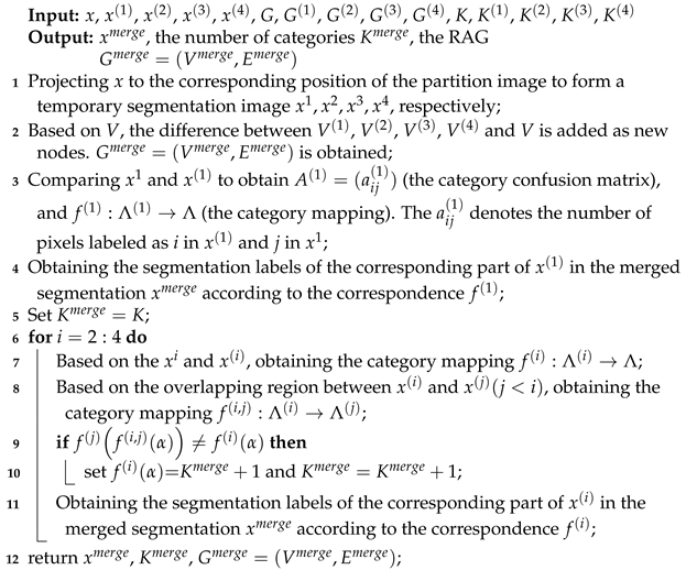
2.3. Rules for Partitioning and Merging

The algorithm OMRF-PGAU proposed in this paper requires first constructing the partitioned image layer $I^{\prime }$. For the given image I, its pixel location index set is $S^{pixel}=\left\{\left(m,n\right)\left|1\le m\le M,1\le n\le N\right.\right\}$. The set of pixel point location indexes for $I^{\prime }=\{I^{\left(1\right)},$$I^{\left(2\right)},I^{\left(3\right)},I^{\left(4\right)}\}$ can be written as,

$$S^{pixel\left(i\right)}=\left\{\left(m^{\prime },n^{\prime }\right)\left|1<m^{\prime }<\frac{M}{2}+\alpha ,1<n^{\prime }<\frac{N}{2}+\alpha \right.\right\}$$

(30)

The pixel position index $\left(m^{\prime },n^{\prime }\right)$ of the partitioned image $I^{\left(i\right)}$ has the following mapping relationship with the pixel position index $(m,n)$ of the original image I. And the $\alpha$ is the length of the overlapping area between the partition images.

$$f\left(m^{\prime },n^{\prime },i\right)=\left(m,n\right)=\left(m^{\prime }+\xi \left(i\right)·\left(\frac{M}{2}-\alpha \right),n^{\prime }+\zeta \left(i\right)·\left(\frac{N}{2}-\alpha \right)\right)$$

(31)

$$\xi \left(i\right)=\left\{\begin{array}{cc}1& i\in \left\{3,4\right\}\\ 0& else\end{array}\right.,\zeta \left(i\right)=\left\{\begin{array}{cc}1& i\in \left\{2,4\right\}\\ 0& else\end{array}\right.$$

(32)

In the updating process, the auxiliary segmentation results of the partition images, $x^{part}=\left\{x^{part\left(1\right)},x^{part\left(2\right)},x^{part\left(3\right)},x^{part\left(4\right)}\right\}$, need to be constructed from x:

(1) The segmentation result of the original image is first mapped to the corresponding position of each partitioned image, i.e.,

$$x_{m^{\prime },n^{\prime }}^{part\left(i\right)}=x_{f\left(m^{\prime },n^{\prime },i\right)}$$

(33)

(2) Based on $G=\left(V,E\right)$ and $G^{\left(i\right)}=\left(V^{\left(i\right)},E^{\left(i\right)}\right)$, the difference between V and $V^{(}i)$ is added as new nodes. The RAG of the auxiliary segmentation can be obtained, $G^{part\left(i\right)}=\left(V^{part\left(i\right)},E^{part\left(i\right)}\right)$.

(3) The auxiliary segmentation labels of the nodes in $I^{\left(i\right)}$ are obtained, i.e.,

$$x_{s^{\prime }}^{part\left(i\right)}=\mathrm{mode}\left(\left\{x_{m^{\prime },n^{\prime }}^{part\left(i\right)}\left|\left(m^{\prime },n^{\prime }\right)\in V_{s^{\prime }}^{part\left(i\right)}\right.\right\}\right)$$

(34)

The $\mathrm{mode}\left(A\right)$ denotes the operation of taking the mode of the set A.

Regarding the $X^{merge}$ in Equation (22), it represents the auxiliary segmentation of the original image obtained from the segmentation results of four partition images by the merging algorithm (Algorithm 1). The merging algorithm (Algorithm 1) is shown below.

Algorithm 1: Merging algorithm for segmentation results of partitioned images.

2.4. Update Path of the OMRF-PGAU

Equations (21) and (22) are the derivations of the prior probabilities of the label fields for the original and partitioned images. Equation (29) represents the update path of the segmentation result in the cycle. Specifically, in each update cycle, there exists a circular update path as shown in the dashed box in Figure 2.

(1) In the t-th cycle, the original image is updated independently, i.e., without considering the effect of the segmentation of the partitioned image on it, and the segmentation result $x^{temp}$ is obtained:

$$x^{temp}=\underset{x}{argmax}P\left(Y=y\left|X=x\right.\right)·P\left(X=x\right)$$

(35)

$$x_s^{temp}=\underset{x_s}{argmax}P\left(Y_s=y_s\left|X_s^t=x_s\right.\right)·P\left(X_s^t=x_s\left|X_{N_s}^{t-1}=x_{N_s}^{t-1}\right.\right)$$

(36)

(2) The $x^{temp}$ is projected to the partition images as the auxiliary segmentation $x^{part,t}=\left\{x^{part\left(1\right),t},x^{part\left(2\right),t},x^{part\left(3\right),t},x^{part\left(4\right),t}\right\}$ according to the partitioning rules as Section 2.4 shown.

(3) Combined with the auxiliary label segmentation $x^{part,t}$, the segmentation results of each partitioned image, ${x^{\prime }}^{temp}=\left\{x^{\left(1\right),temp},x^{\left(2\right),temp},x^{\left(3\right),temp},x^{\left(4\right),temp}\right\}$ are updated.

$$x^{\left(i\right),temp}=\underset{x^{\left(i\right)}}{argmax}P\left(Y^{\left(i\right)}=y^{\left(i\right)}\left|X^{\left(i\right),temp}=x^{\left(i\right)}\right.\right)·P\left(X^{\left(i\right),temp}=x^{\left(i\right)}\left|X^{part\left(i\right),t}=x^{part\left(i\right),t}\right.\right)$$

(37)

$$\begin{array}{cc}\hfill x_{s^{\prime }}^{\left(i\right),temp}=\underset{x_{s^{\prime }}^{\left(i\right)}}{argmax}& P\left(Y^{\left(i\right)}=y^{\left(i\right)}\left|X_{s^{\prime }}^{\left(i\right),temp}=x_{s^{\prime }}^{\left(i\right)}\right.\right)·P\left(X_{s^{\prime }}^{\left(i\right),temp}=x_{s^{\prime }}^{\left(i\right)}\left|X_{N_{s^{\prime }}^{\left(i\right)}}^{\left(i\right)}=x_{N_{s^{\prime }}^{\left(i\right)}}^{\left(i\right),t-1}\right.\right)\hfill \\ \hfill & ·P\left(X_{s^{\prime }}^{\left(i\right),temp}=x_{s^{\prime }}^{\left(i\right)}\left|X_{N_{s^{\prime }}^{p\left(i\right)}}^{part\left(i\right),t}=x_{N_{s^{\prime }}^{p\left(i\right)}}^{part\left(i\right),t}\right.\right)\hfill \end{array}$$

(38)

(4) The ${x^{\prime }}^{temp}$ is taken as the prior segmentation result to update the four partitioned images separately and independently, i.e., without considering the influence of the segmentation results of other images. The obtained segmentation results of the four partitioned images are noted as ${x^{\prime }}^t=\left\{x^{\left(1\right),t},x^{\left(2\right),t},x^{\left(3\right),t},x^{\left(4\right),t}\right\}$.

$$x^{\left(i\right),t}=\underset{x^{\left(i\right)}}{argmax}P\left(Y^{\left(i\right)}=y^{\left(i\right)}\left|X^{\left(i\right),t}=x^{\left(i\right)}\right.\right)·P\left(X^{\left(i\right),t}=x^{\left(i\right)}\right)$$

(39)

$$x_{s^{\prime }}^{\left(i\right),t}=\underset{x_{s^{\prime }}^{\left(i\right)}}{argmax}P\left(Y^{\left(i\right)}=y^{\left(i\right)}\left|X_{s^{\prime }}^{\left(i\right),t}=x_{s^{\prime }}^{\left(i\right)}\right.\right)·P\left(X_{s^{\prime }}^{\left(i\right),t}=x_{s^{\prime }}^{\left(i\right)}\left|X_{N_{s^{\prime }}^{\left(i\right)}}^{\left(i\right),temp}=x_{N_{s^{\prime }}^{\left(i\right)}}^{\left(i\right),temp}\right.\right)$$

(40)

(5) The ${x^{\prime }}^{t1}$ is merged into the original image size as the auxiliary label segmentation $x^{merge,t}$ according to the merging algorithm shown in Section 2.4.

(6) According to Assumption 3, the labeled field of the original image take $x^{temp}$ and $x^{merge,t}$ as prior knowledge, and the segmentation result $x^t$ of the original image can be updated.

$$x^t=\underset{x}{argmax}P\left(Y=y\left|X^t=x\right.\right)·P\left(X^t=x\left|X^{merge,t}=x^{merge,t}\right.\right)$$

(41)

$$x_s^t=\underset{x_s}{argmax}P\left(Y_s=y_s\left|X_s^t=x_s\right.\right)·P\left(X_s^t=x_s\left|X_{N_s}^{temp}=x_{N_s}^{temp}\right.\right)·P\left(X_s^t=x_s\left|X_{N_s^m}^{merge,t}=x_{N_s^m}^{merge,t}\right.\right)$$

(42)

The overall algorithm of the OMRF-PGAU is given below (Algorithm 2). In this paper, the mean shift algorithm [48] is used as an over-segmentation algorithm to obtain the RAGs of images.

Algorithm 2: Framework of the OMRF-PGAU model.

3. Experiments

In this section, OMRF-PGAU is experimentally verified for the performance of the method and compared with some other state-of-the-art MRF-based methods. First, the high spatial resolution remote sensing image database used in the experiment and the indicators to measure the performance of the methods are introduced. Then the robustness experiments of each parameter of the OMRF-PGAU method will be conducted to determine the range of the parameters. Finally, a comparison with other MRF-based methods will be made and the quantitative index of the segmentation results will be given. All experiments in this article are run on personal laptop. The operating system is Windows 10 (Microsoft (China) Co., Ltd., Beijing, China), and the experimental software is Matlab R2020a (Mathworks, Natick, Massachusetts 01760 USA). Hardware information is as follows, CPU: i7-9750H, GPU: GTX-1660Ti, RAM: 32GB(DDR4 2666MHz), ROM: 512GB(SSD) + 2TB(HHD). In this section, we first set up experiments on the parameters of the proposed model, and the results are shown in Figure 3, Figure 4 and Figure 5. After that, we conduct segmentation comparison experiments on synthetic images (Figure 6, Figure 7 and Figure 8) and natural remote sensing images (Figure 9, Figure 10, Figure 11, Figure 12, Figure 13, Figure 14, Figure 15, Figure 16 and Figure 17) respectively. The details of the experiments will be provided next.

3.1. Datasets and Evaluation

3.1.1. Datasets

To verify the effectiveness of the algorithm proposed in this article, we selected different types of mosaic images and remote sensing images (from four different databases). In particular, the three mosaic images are the color texture mosaic and the wood texture mosaic, as shown in Figure 6, Figure 7 and Figure 8, which are generated by the Prague texture segmentation data generator [49]. The sizes of the images both are 512 × 512. Three images selected from the SPOT5 remote sensing database are shown in Figure 9, Figure 10 and Figure 11. The sizes are 560 × 420, 1000 × 1600, 1600 × 1600, respectively. The spatial resolution is 10 m. Three images from Gaofen Image Dataset (GID) [50], as shown in Figure 12, Figure 13 and Figure 14. The image sizes are 1400 × 2200, 1800 × 1800 and 3000 × 3000, the spatial resolution is 3.2 m. There are three near-ground aerial images taken in Taizhou are shown in Figure 15, Figure 16 and Figure 17, the sizes are 1024 × 1024, 2240 × 2240, 5000 × 5000, and the spatial resolution is 0.4 m, 0.1 m, 0.1 m.

3.1.2. Evaluation Indicator

In order to objectively evaluate the accuracy of the segmentation results and give an objective evaluation numerically, this paper uses remote sensing images to divide the evaluation indicators Kappa and overall accuracy (OA) [51], which are commonly used in various fields. These two indicators are based on the confusion matrix $CM={\left(M_{ij}\right)}_{k\times k}$, where $M_{i}j$ represents the number of pixels that actually belong to the i-th category but are classified into the j-th category in the segmentation result. The calculation formula of Kappa and OA is as follow:

$$Kappa=\frac{M·{\displaystyle \sum _{i=1}^k}{M}_{ii}-{\displaystyle \sum _{i=1}^k}\left(M_{i+}·M_{+i}\right)}{M^2-{\displaystyle \sum _{i=1}^k}\left(M_{i+}·M_{+i}\right)},OA=\frac{{\displaystyle \sum _{i=1}^k}{M}_{ii}}{M}$$

(43)

In Equation (43), $M={\displaystyle \sum _{i=1}^k}{\displaystyle \sum _{j=1}^k}{M}_{ij}$, $M_{i+}={\displaystyle \sum _{j=1}^k}{M}_{ij}$, $M_{+i}={\displaystyle \sum _{j=1}^k}{M}_{ji}$. For different segmentation results of the same image, the higher the value of $\kappa$ and OA, the closer to the reality, the better the performance of the algorithm.

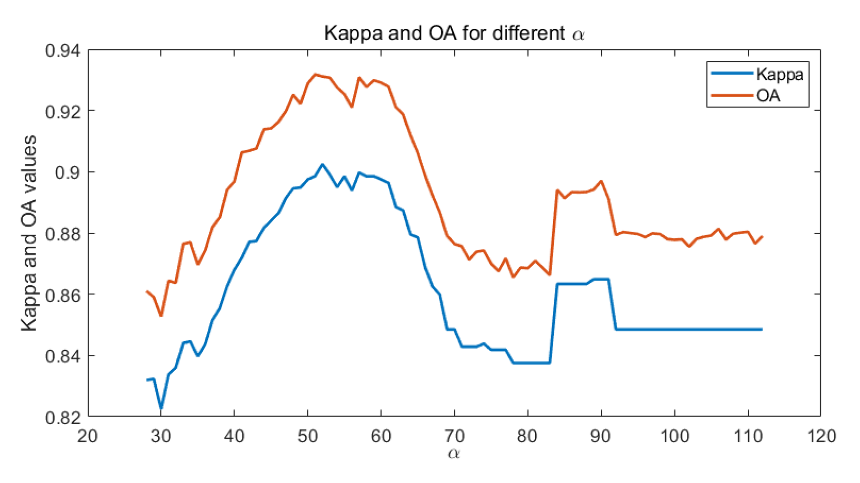
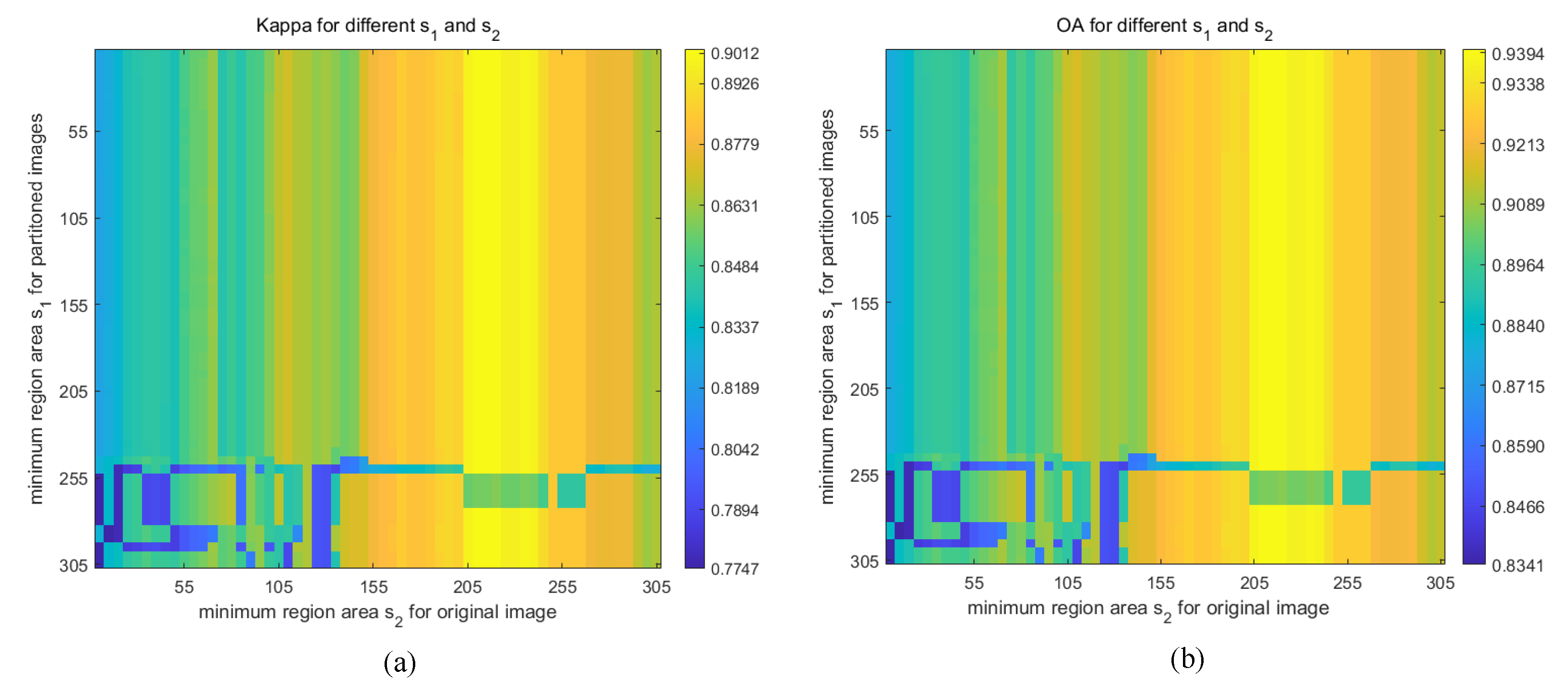
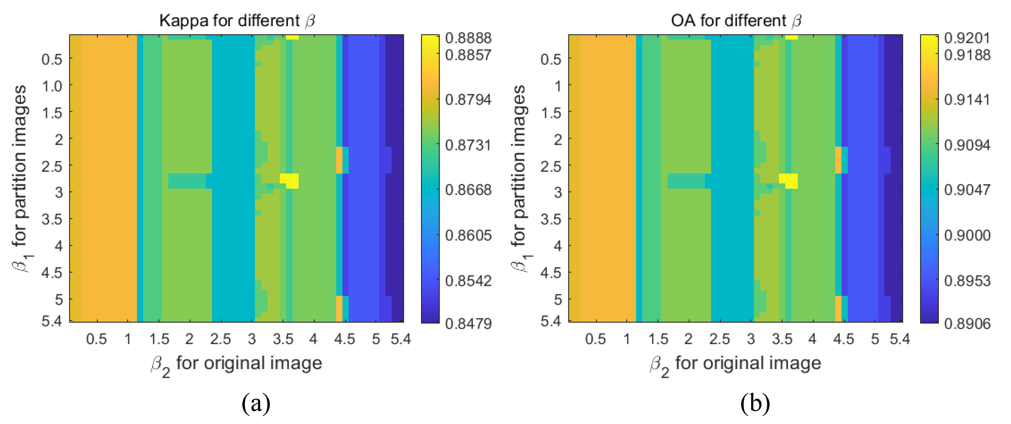
3.2. Robustness of Parameter in OMRF-PGAU

In the OMRF-PGAU algorithm, the input parameters mainly include the following: the length of the overlapping area between the partition images ($\alpha$), the minimum region area of over-segmented algorithm for each image ($s_1,s_2$), and the parameter of the potential energy function of the label field of each image (${\beta }_1,{\beta }_2$).

The length of overlap area is mainly used in the algorithm to calculate the corresponding relationship of each partition image category. If the length is too small, the corresponding relationship will be unreliable due to too little sample data; if the length is too large, the amount of the calculation will increase, and the difference between the partition image and the original image will become smaller, and iteratively optimize no significant effect. To verify the setting range of the length parameter for the overlap area, take the Figure 9a as the experimental object. The size of the image is 560 × 420, so we set the $\alpha$ value from 28 (5% of the original image length) to 112 (20% of the original image length) of the original image size, the step size is 2 (0.357% of the original image length), and uses Kappa and OA as the evaluation indicators, as shown in Figure 3. It can be seen that, when the length of overlap area is in the [50, 60] (8.9∼10.7% of the original image length), the impact on the segmentation result is small, and the segmentation performance is better. Therefore, in the subsequent experiments of this article, the default value of the regional coincidence parameter is selected as 8.9∼10.7% of the original image length, which will be fine-tuned for different images.

In this paper, the mean-shift algorithm [48] is used to obtain the granularity results of each image. The minimum region area can determine the size of the over-segmented region in the image in order to obtain different granularities. Different regional features can be extract based on different granularities, and the calculation results of the potential energy function in the label field can be also effected. We take Figure 9a as the experimental object, different minimum region areas are set to test the effect of this parameter on the performance of the OMRF-PGAU algorithm. The value of $s_1$ (minimum region area for the partition images) and $s_2$ (minimum region area for the original image) ranges from 10 to 305, and the step size is 5. The Kappa and OA of the segmentation results under each value are shown in the Figure 4. It can be seen that compared to the minimum area parameter $s_1$ of the partition images, the segmentation result is mainly affected by the minimum area parameter $s_2$ of the original image. When the $s_2$ between 200∼240 (0.0850∼0.1020% of the image area), the result is more stable, and the performance is better than other values. So in this paper, we set the $s_1$ and $s_2$ as 0.09% of the image area, which will be fine-tuned for different images.

The parameter in the potential energy function of the label field is also a parameter that needs to be manually set. It is mainly responsible for balancing the energy effect between the label field and the feature field. If the $\beta$ is too small, the segmentation result is mainly affected by the energy of the feature field, and the spatial relationship of each node will be ignored; if it is set too large, the spatial relationship will be emphasized, and the feature of each node will be ignored. In our proposed method, there are 5 images (original image and four partition images). We set the ${\beta }_1$ of the partition images to be consistent, and ${\beta }_2$ for the original image. These two parameters are set from 0.1 to 5.4, and the step is 0.1. We use the Kappa and OA to measure the quality of the segmentation results. The evaluation of the segmentation results for different $\beta$ values is shown in the Figure 5. It can be seen that compared to the potential energy parameter ${\beta }_1$ of the partitioned image, the segmentation result is mainly affected by the potential energy parameter ${\beta }_2$ of the original image. For the ${\beta }_2$, in the interval (0.1,1.3), the result is relatively stable, and the OMRF-PGAU performs better when the ${\beta }_1$ around 3 and ${\beta }_2$ around 3.5. Thus, in the following experiments, in order to ensure the stability, we set ${\beta }_1$ around 3, ${\beta }_2$ in the interval (0.4,0.9).

In short, although the proposed algorithm, OMRF-PGAU, contains many parameters, some of the parameters in the calculation process, such as Gaussian distribution parameters, can be set according to statistical principles; and the numerical parameters need to be manually given, such as the $\alpha$, the minimum region area, and the potential energy parameter, there is a relatively stable value range for the segmentation result.

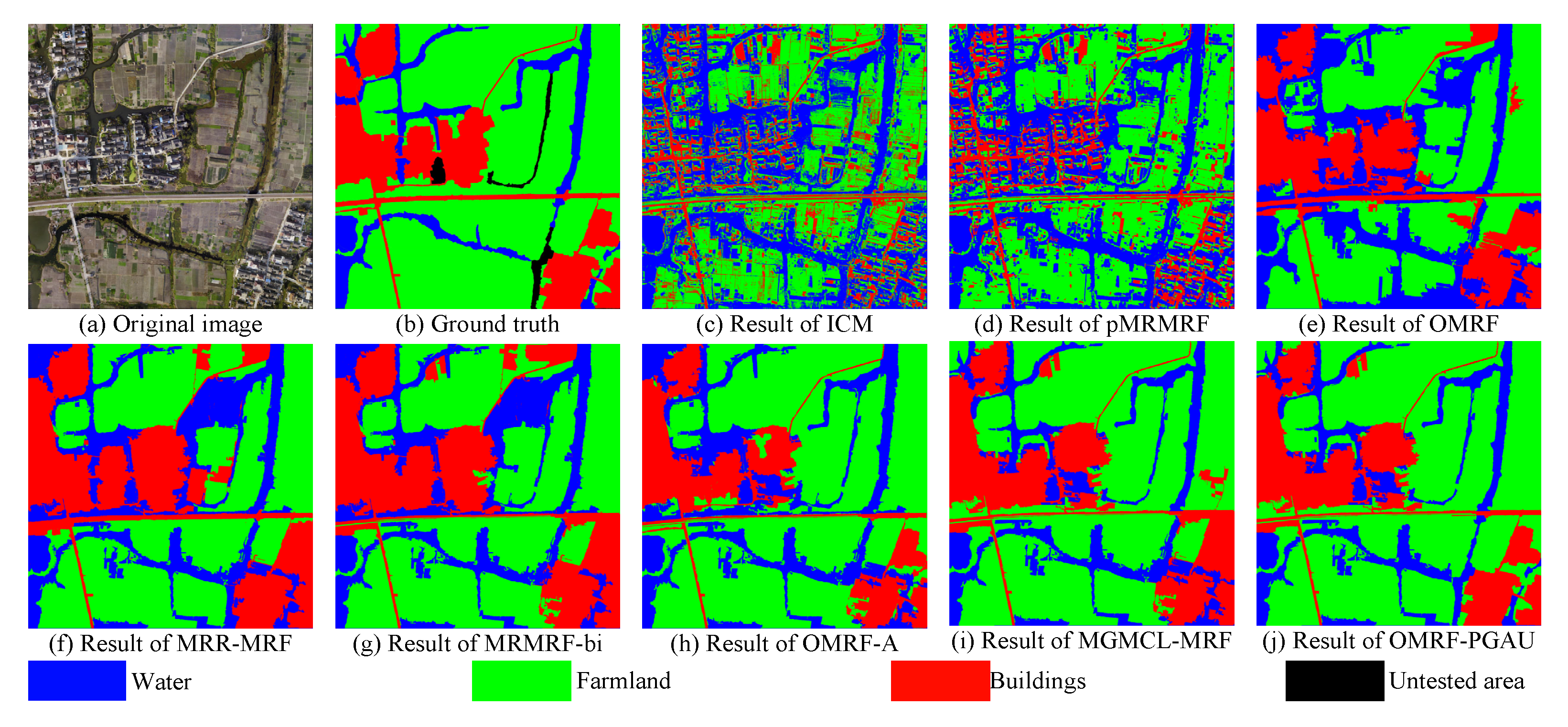
3.3. Comparison Methods

To further verify the effectiveness of the proposed algorithm, there are some MRF-based methods selected for comparative experiments, namely:

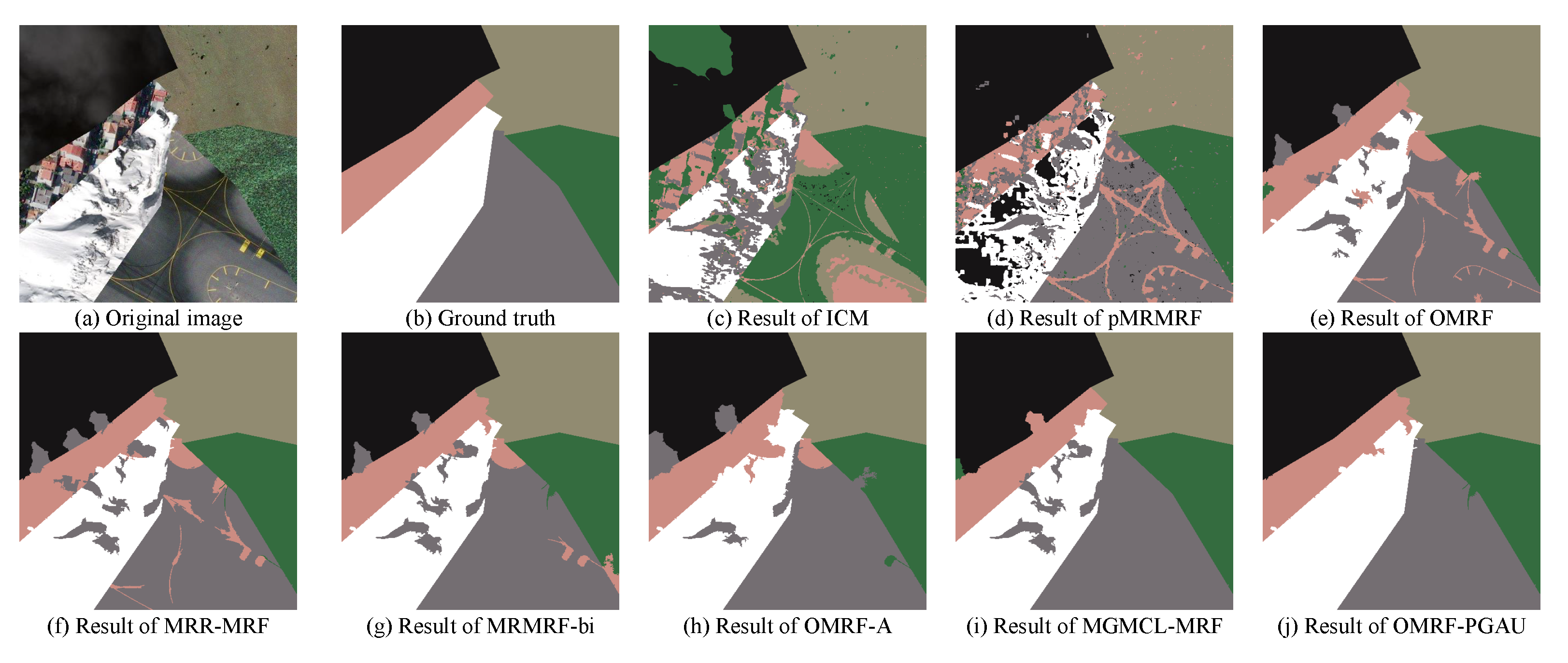
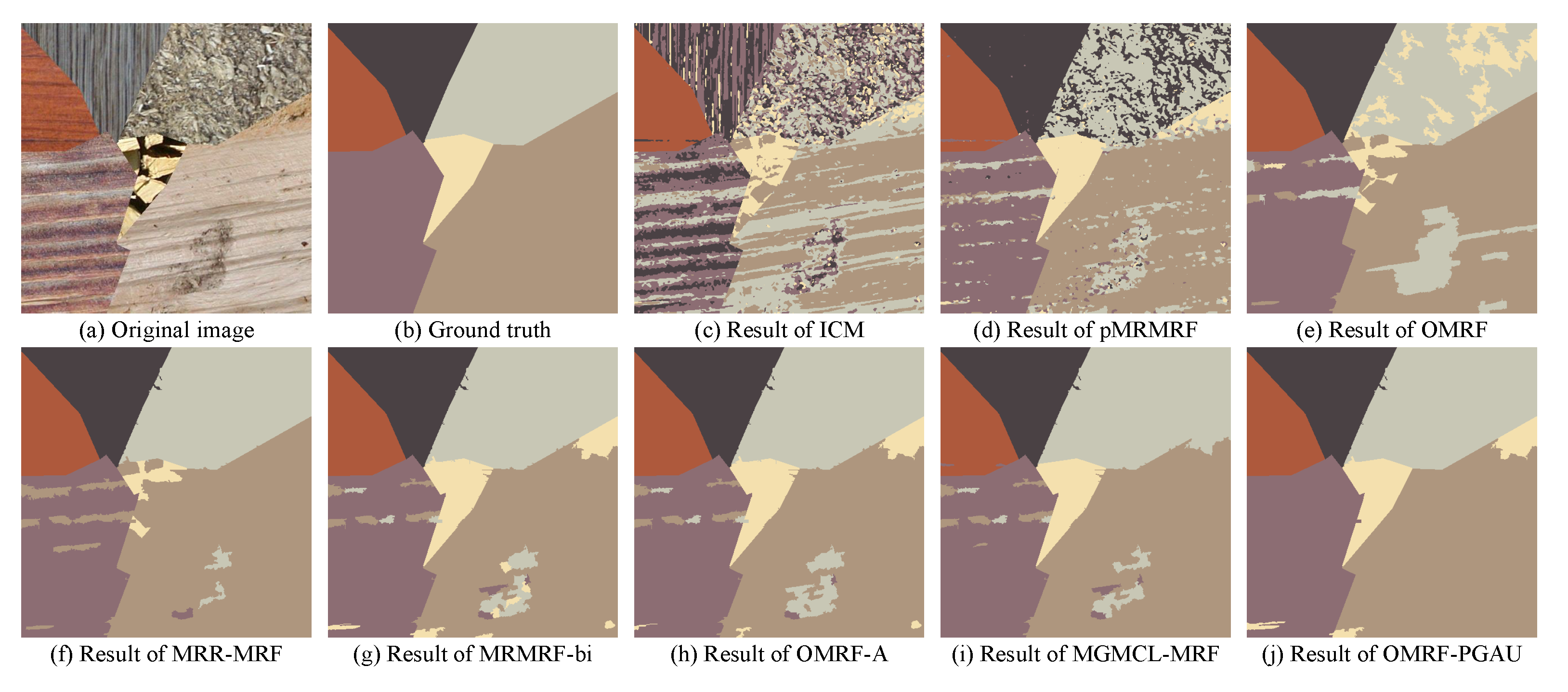
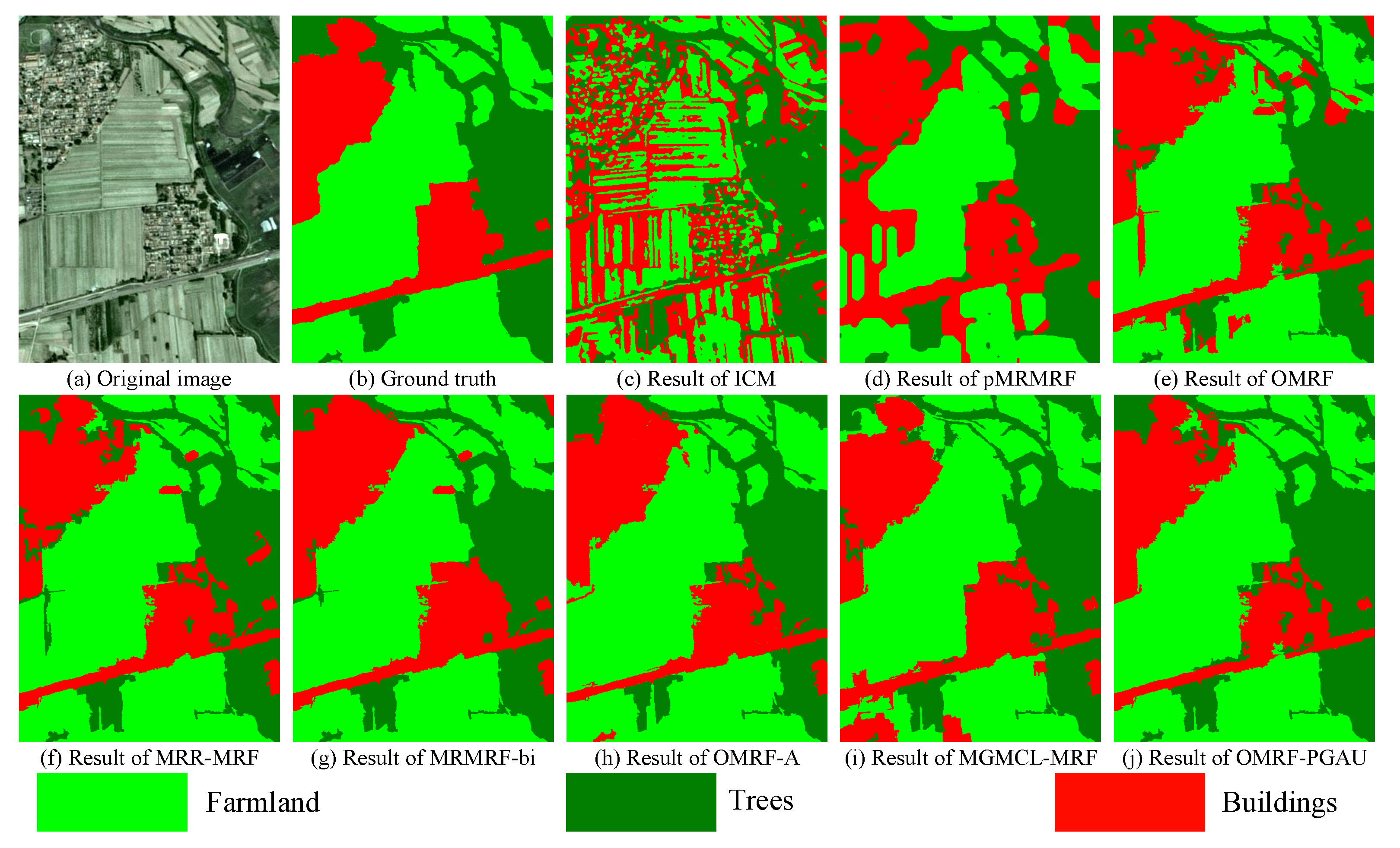
• ICM [27]: the classic pixel-level Markov random field model, which uses pixels as nodes to model and update the segmentation results;
• pMRMRF [43]: introduces wavelet transform, constructs multi-resolution layers, constructs pMRF model in each layer, and updates and transfer the segmentation results from top to bottom. The upper layer’s segmentation is directly projected to the lower layer as the initial segmentation;
• OMRF [46]: the over-segmentation algorithm first obtains a series of homogeneous regional objects and uses them as nodes to construct an MRF model;
• MRR-MRF [28]: on the basis of pMRMRF, each layer is modeled by OMRF to form an MRF model of multi-regional granularity and multi-resolution layers;
• MRMRF-bi [44]: on the basis of pMRMRF, the original image is modeled by OMRF, and the area objects are projected to all layers. Each layer is updated from the top to bottom, and the impact of the adjacent upper and lower layer segmentation results on this layer is also considered when updating;
• OMRF-A [29]: on the basis of OMRF, an auxiliary mark field is introduced to construct a hybrid segmentation mark, and the low semantic layer and the high semantic layer are used to assist in the update of the segmentation results of the original semantic layer;
• MGMCL-MRF [32]: it develops a framework that builds a hybrid probability graph on both pixel and object granularities and defines a multiclass-layer label field with hierarchical semantic over the hybrid probability graph.

By comparing with the above methods, the difference between the proposed algorithm and different types of MRF-based methods can be obtained. Among the above methods, there is MRF defined on the single layer method (ICM and OMRF), MRF defined on multiple auxiliary layers (pMRMRF, MRR-MRF, MRMRF-bi), MRF defined on single granularity with multi-class (OMRF-A), and MRF defined on multi-granularity with multi-class (MGMCL-MRF).

For the sake of fairness, all object-based algorithms use the mean-shift method to obtain the result of over-segmentation regions, and the minimum region area is set to 0.9% of the experimental image area. For multi-resolution methods, wavelet transform is used for low-resolution sampling, and “Haar” wavelet is used to construct a three-layer multi-resolution structure. The setting of the $\beta$ (potential energy function parameter) of all MRF methods adopts the value range described in the previous subsection. The category number settings of the multi-class method refer to the settings of the paper to which it belongs.

3.4. Segmentation Experiments

The effectiveness of the OMRF-PGAU algorithm for texture processing is first verified on the texture image images, because most of the ground objects in remote sensing images have certain texture characteristics. For real RGB remote sensing images, the effectiveness of the OMRF-PGAU algorithm for semantic segmentation of high spatial resolution images is verified by testing images of different high spatial resolutions, different image sizes, and different semantic categories of features.

3.4.1. Segmentation for Texture Images

Remote sensing images are rich in textures. Therefore, we first tested on synthetic texture images to verify the effectiveness of the algorithm proposed in this paper. The three synthetic texture images, as shown in Figure 6a, Figure 7a and Figure 8a, were both generated by the Prague texture segmentation data generator.

These three images are both sized 512 × 512, and contain six category textures. For the Figure 6a, the two types textures on the left-lower have greater similarities in the RGB channels. For the textures in the upper-left, lower-left, upper- right, and lower-right parts, the RGB channels of the same type are obviously different. As for the Figure 7a, its six textures are composed of GeoEye images. The town texture on the left is composed of red roofs and black shadows, the airstrip on the lower-right has a larger range of RGB spectrum value changes, and most of them are similar to the upper-left texture. In the Figure 8a, there are six wood textures, and the three types on the left contain striped structures, the RGB distribution of the two types on the right and the one in the middle are quite different. These are great challenges for semantic segmentation. The segmentation results are shown in the Figure 6, Figure 7 and Figure 8.

Table 1. Quantitative indicators of eight comparison methods for two texture images.

Methods		ICM	pMRMRF	OMRF	MRR-MRF	MRMRF-bi	OMRF-A	MGMCL-MRF	OMRF-PGAU
Figure 6	Kappa	0.6218	0.6658	0.7742	0.7991	0.8348	0.8521	0.8779	0.9527
	OA	0.6596	0.7039	0.8053	0.8274	0.8590	0.8742	0.8974	0.9607
Figure 7	Kappa	0.5350	0.8086	0.9192	0.9327	0.9193	0.9289	0.9582	0.9916
	OA	0.5706	0.8344	0.9320	0.9437	0.9321	0.9405	0.9654	0.9931
Figure 8	Kappa	0.5046	0.7978	0.8331	0.9277	0.9317	0.9355	0.9499	0.9761
	OA	0.5467	0.8298	0.8633	0.9440	0.9459	0.9490	0.9608	0.9816

shows the accuracy evaluation indexes of each method for the semantic segmentation results of Figure 6a, Figure 7a, and Figure 8a.

From the segmentation results, for Figure 6a, it is the phenomenon that the same type of texture contains different features, which causes the poor segmentation performance of the two pixel-level MRF methods (ICM, pMRMRF). The segmentation results of object-level methods have been significantly improved, but there are all misclassifications. Among them, OMRF divides the lower left texture into three parts, the lower right part is divided into two parts, and most of the lower left and middle lower parts are divided into the same type. The two multi-layer structures (MRR-MRF and MRMRF-bi) have improved compared to the single-layer structure. Because they can get spatial information of different scales in different resolution layers. However, there are still problems with OMRF. The two multi-category methods have significantly improved the results of image segmentation. This is because they introduce multi-category auxiliary markers, which can reasonably mine the sub-categories contained in various textures and improve the segmentation accuracy. The OMRF-A method distinguishes between the lower left and middle left textures, but the lower right texture has a significant misclassification phenomenon. MGMCL-MRF can distinguish five kinds of textures more accurately, and the lower right part is segmented relatively completely, but the texture misclassification in the lower left part is serious. The segmentation result of OMRF-PGAU performs better than the selected comparison method. The six textures are basically distinguished, but there are still a small amount of misclassification in the lower right part, mainly because the RGB distribution within the texture varies widely.

As for the Figure 7a, since the node considered by the ICM method is a pixel, and the neighborhood only contains eight surrounding pixels, the spatial relationship considered is relatively narrow, so the segmentation result is obviously misclassified. Because MRMRF constructs a multi-resolution layer structure, a larger range of spatial relationships can be considered, so the segmentation results have been improved. Several object-level methods use over-segmented regions as nodes in the probability graph, so the regional consistency of the segmentation results is better, and the completeness of each category of the segmentation results is higher. Among them, MRR-MRF and MRMRF-bi combine object-level idea and multi-resolution scales to significantly improve the segmentation of urban parts. OMRF-A and MGMCL-MRF use multiple label fields to segment the airstrips part more completely. OMRF-PGAU uses the partitioning-the overall alternate update mechanism, combined with the advantages of the auxiliary label field, so that the segmentation accuracy of towns, snow-capped mountains and airstrips is better.

In the Figure 8a, there are two parts in the lower right category that are quite different from the surrounding ones. The middle category includes both wood and wood shadows. For the three categories on the left, they all contain a large number of clauses and structures. We can see the result that the pixel-level segmentation algorithm cannot solve the problem of the classification of the strip structure. The segmentation accuracy of object-level algorithms has been significantly improved. The classification accuracy of the three categories on the left is gradually improved. Among them, the algorithm proposed in this article has the best performance. This is because, in the partition auxiliary images, some only contain two categories, and the complex multi-classification problem is transformed into a relatively simple small-number classification problem. After the partition and merging algorithm is used to obtain the category correspondence, it can have a higher classification accuracy.

3.4.2. Segmentation for SPOT Images

To verify the segmentation performance of the OMRF-PGAU method for real remote sensing images, in this section, two SPOT5 satellite images are selected as experimental objects. The first image is 560 × 420 in size and contains three types of objects, buildings, farmland, and trees. The second image has a size of 1000 × 1600 and contains only two categories of objects, buildings, and farmland. The third image has a size of 1600 × 1600 and contains four types of objects, buildings, farmland, water, and trees. The spatial resolution of three images is 10 m. The segmentation results of the three images by each method are shown in Figure 9, Figure 10 and Figure 11, and the evaluation indicators of the segmentation results are shown in

Table 2. Quantitative indicators of eight comparison methods for three SPOT5 images.

Methods		ICM	pMRMRF	OMRF	MRR-MRF	MRMRF-bi	OMRF-A	MGMCL-MRF	OMRF-PGAU
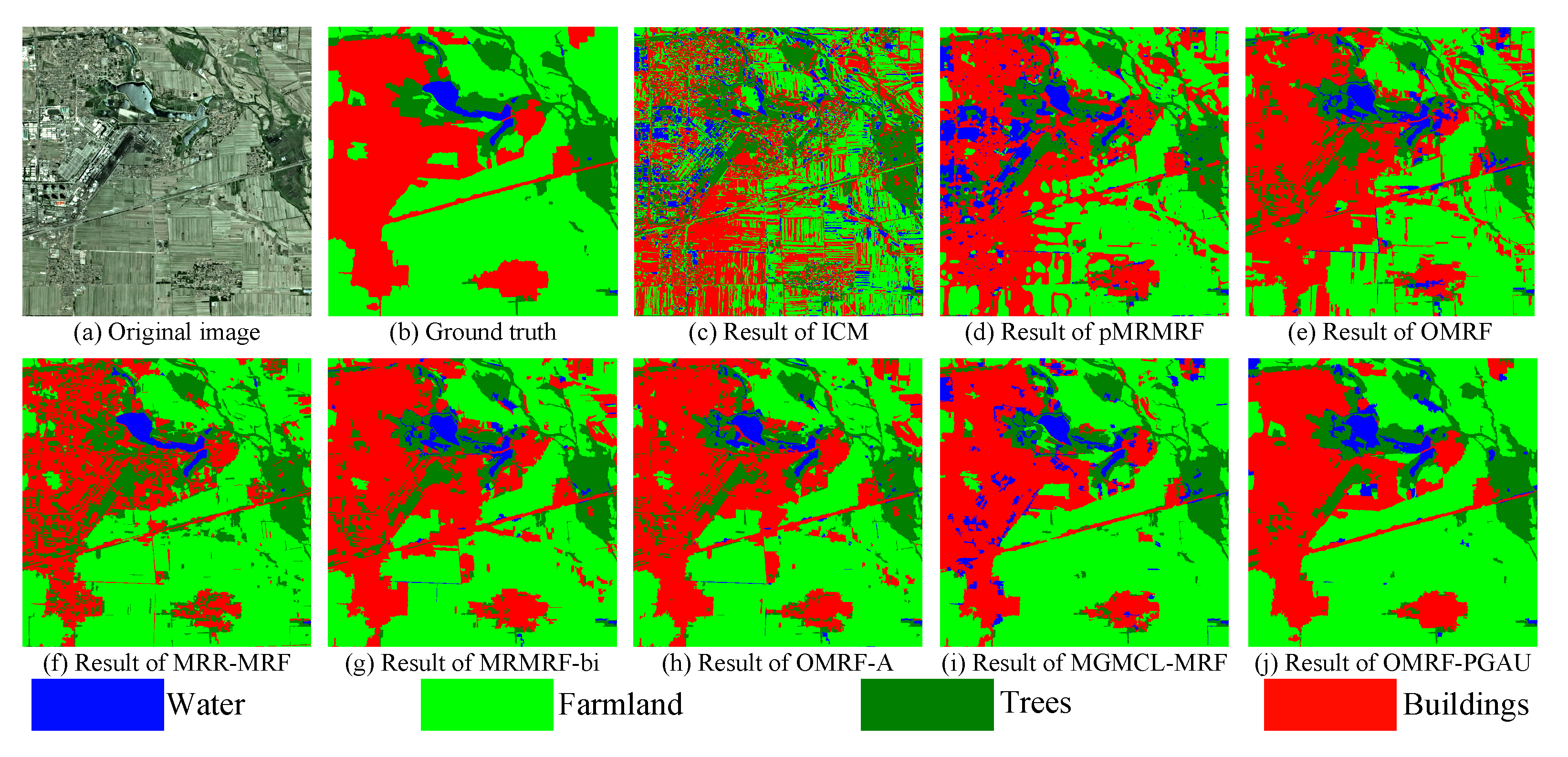
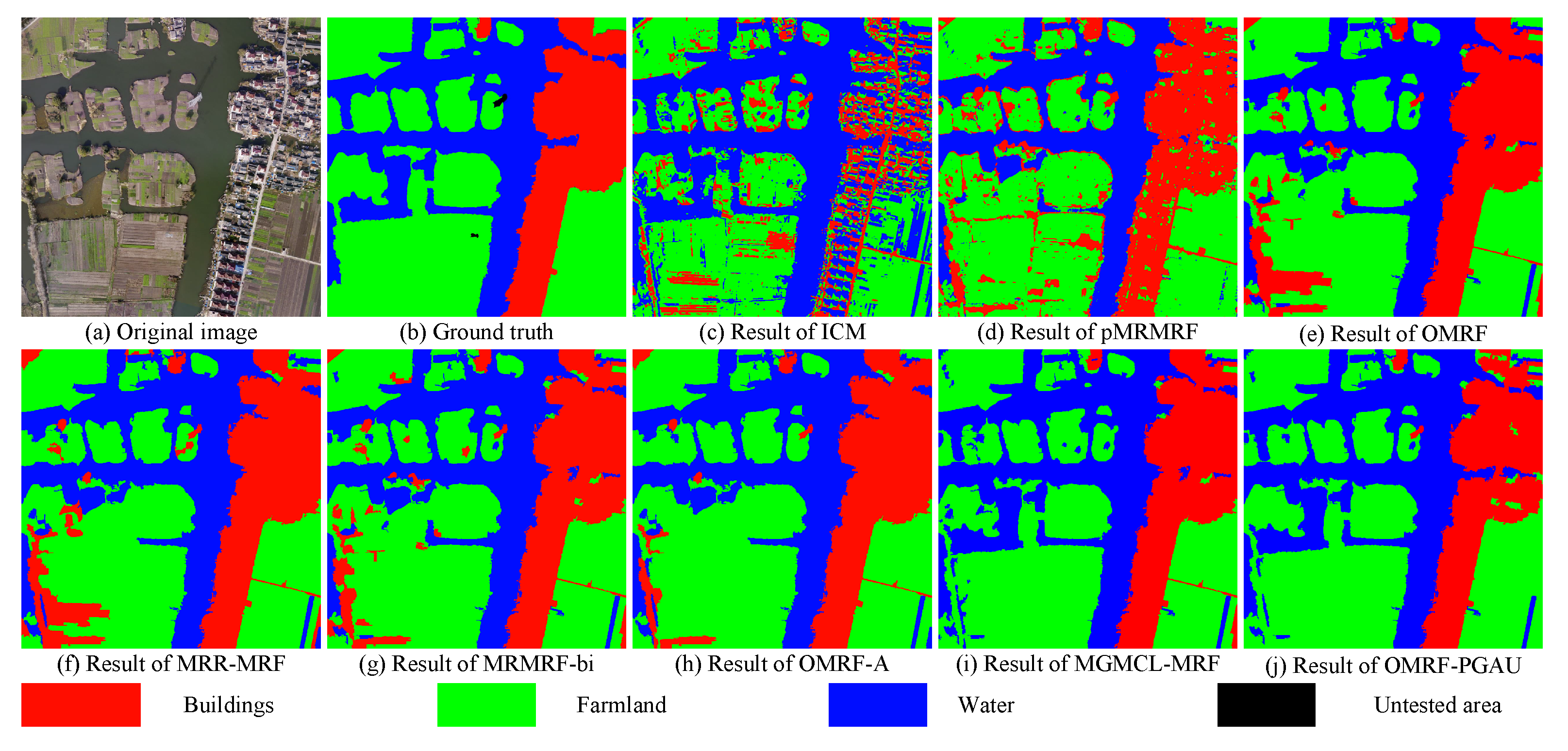
Figure 9	Kappa	0.5656	0.7656	0.8343	0.8618	0.8650	0.8733	0.8685	0.8836
	OA	0.6451	0.8232	0.8838	0.9051	0.9076	0.9142	0.9091	0.9213
Figure 10	Kappa	0.6033	0.6416	0.6728	0.6806	0.6809	0.6846	0.6909	0.7436
	OA	0.8095	0.8248	0.8459	0.8510	0.8512	0.8541	0.8597	0.9033
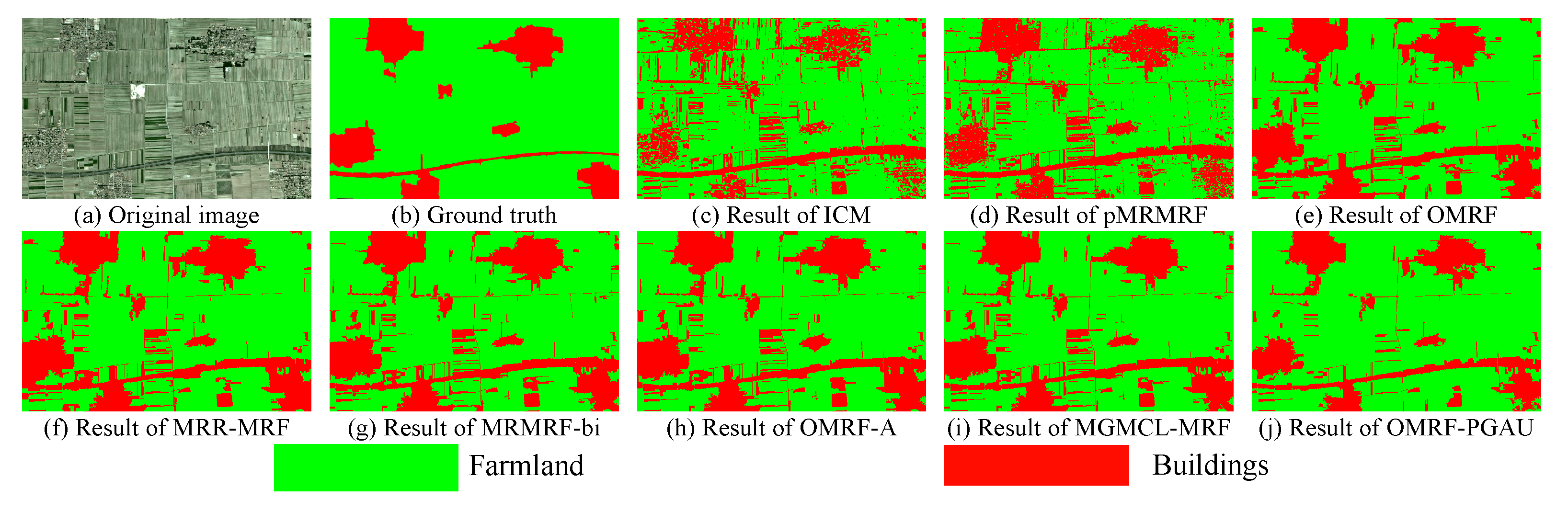
Figure 11	Kappa	0.4191	0.6241	0.6581	0.7398	0.7715	0.7509	0.8440	0.8985
	OA	0.5008	0.6997	0.7306	0.8139	0.8378	0.8192	0.8986	0.9356

.

For Figure 9a, both the urban part and the farmland part contain some trees, moreover, the cultivated land part contains a lot of strip textures, and the overall RGB of the whole image is greenish. These all have a great impact on segmentation. this is a challenge for segmentation. There are many regions of misclassification in the results obtained by ICM, since the pixel-level method can only consider 8-pixel neighbor system. pMRMRF has improved, but a bit too smooth, and the protection of the boundary is very poor, because when the multi-resolution structure is used, the segmentation result is directly expanded twice and projected to a higher resolution layer. This makes pMRMRF’s blurring of borders particularly obvious on small-sized images. The segmentation results of the object-level method are significantly improved. The OMRF and MRR-MRF has some misclassifications mainly in buildings part. Both MRMRF-bi and OMRF-A have a small amount of misclassification in buildings and farmland parts. For the MGMCL-MRF, there are a few misclassifications between buildings and farmland in the lower-left, and there are also a few misclassifications between farmland and trees in the upper-left. The segmentation of OMRF-PGAU is the best, but there is also the phenomenon of misclassification in trees parts.

For Figure 10a, it contains only two categories, buildings and farmland. However, due to the large number of striped structures in the farmland, and the buildings are scattered in the image, they are not concentrated, it is difficult to form a scale effect, so the segmentation is more difficult. From the perspective of segmentation accuracy, the accuracy of each method is not high. Both of the two pixel-level segmentation methods have a large number of salt and pepper misclassification regions, and there are a large number of stripe misclassifications. Object-level algorithms have been improved. Large areas of farmland maintain a high regional consistency. However, it can be seen that they do not improve the misclassification of stripe. This is mainly because the RGB distribution in the farmland area is not concentrated. The algorithm proposed in this paper can extract the buildings well, but for the striped misclassified area in the farmland, compared with other object-level methods, the accuracy is only improved by 5%.

For the Figure 11a, there are many sub-categories in the buildings part, such as: mining area, factory area, residential area, etc.; their spectral values vary widely, and the RGB features of the factory subpart and the trees part are similar. Compared to the entire image, the water part has a small proportion of pixels. All of these have caused a lot of trouble to be segmented. The results of ICM and pMRMRF have many misclassifications in buildings and farmland parts. Since the RGB channel values of the buildings and the farmland are very similar. The black mining area in the buildings part is closer to the spectral feature of the trees part, and all test methods misclassify this part into the trees category except the MGMCL-MRF. MRR-MRF and MRMRF-bi use the multi-resolution structure to obtain more regional information, so the segmentation results are improved, but many pixels of the buildings part are mistakenly classified as trees. The results of MRMRF-bi and OMRF-A mistake a large amount of farmland part in the middle part into the buildings part. MGMCL-MRF improves the misclassification of the middle part, and the mining area is basically divided correctly, this is mainly due to multi-granularity and multi-class labels. The segmentation result of OMRF-PGAU is the best among these several methods. It not only maintains the consistency of the buildings part in the upper-left part, but also ensures that the farmland part in the middle of the image remains independent and not swallowed by the buildings part. This is because the partition-merge alternate update is used to ensure the independence of each small area in the partition image and the regional consistency of each category in the original image.

3.4.3. Segmentation for Gaofen-2 Images

To verify the performance of the proposed algorithm in higher spatial resolution with larger size remote sensing images, the experimental images in this part are two remote sensing images taken from the Gaofen image dataset (GID). The first image is 1400 × 2200, and contains four types of objects, buildings, farmland, water, and trees. The second image has a size of 1800 × 1800 and only contains two types, buildings, and farmland. The third one has a size of 3000 × 3000 and only contains three types, namely buildings, farmland, and water. The spatial resolution of both images is 3.2 m. The segmentation results are shown in Figure 12, Figure 13 and Figure 14, and the accuracy measurement indexes of the segmentation results are shown in

Table 3. Quantitative indicators of eight comparison methods for three Gaofen-2 images.

Methods		ICM	pMRMRF	OMRF	MRR-MRF	MRMRF-bi	OMRF-A	MGMCL-MRF	OMRF-PGAU
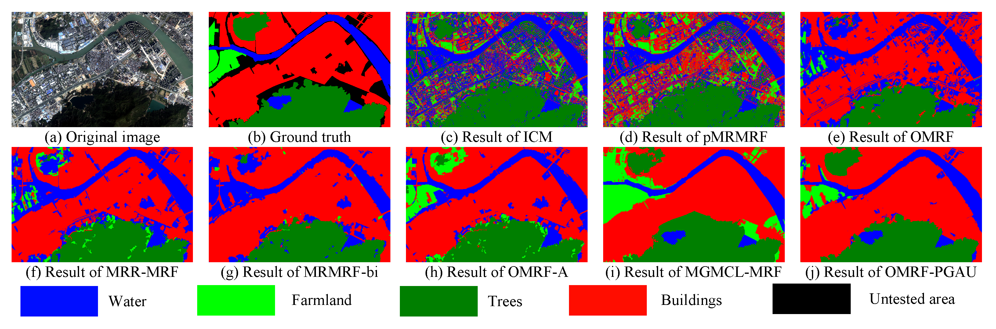
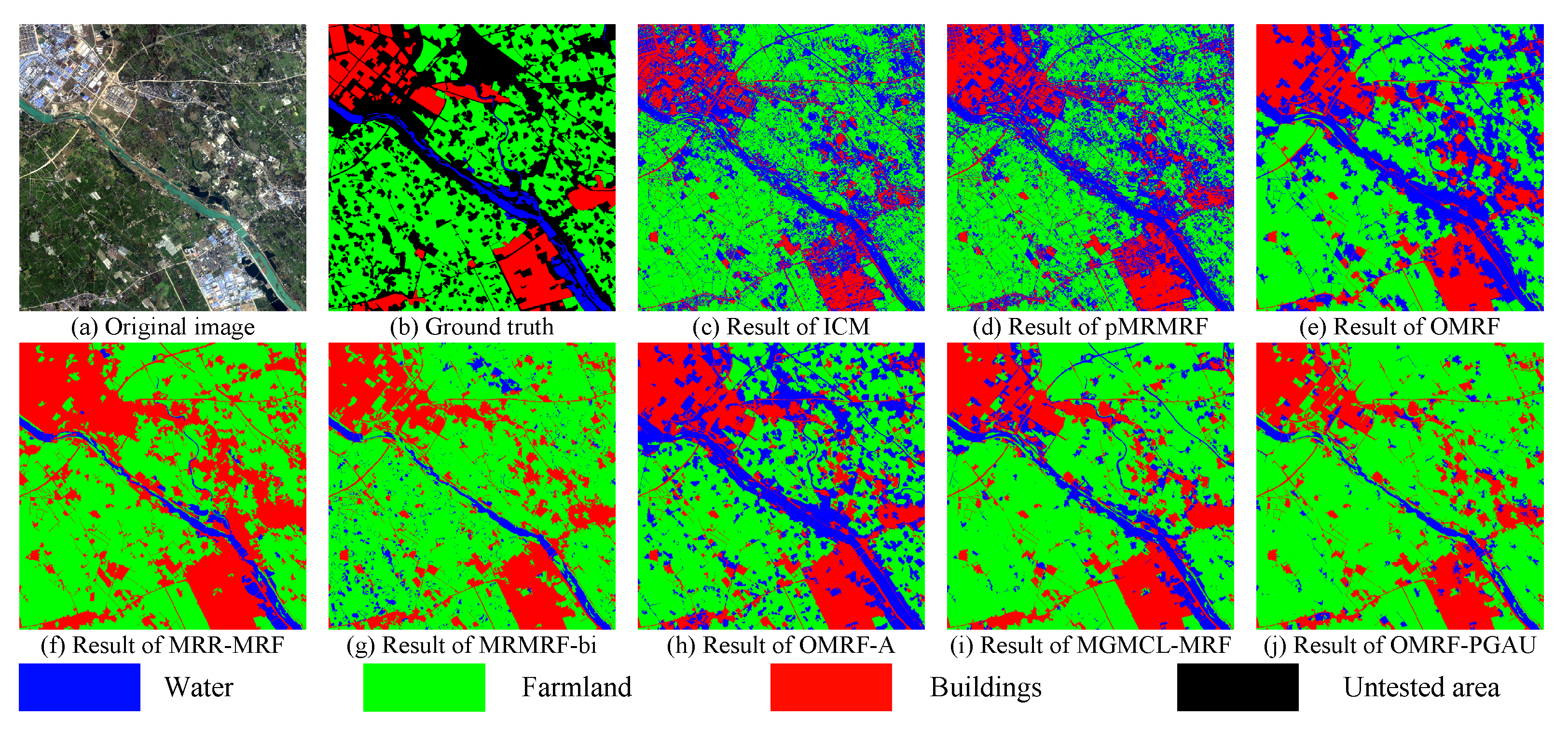
Figure 12	Kappa	0.4687	0.5588	0.7429	0.8050	0.7966	0.8849	0.9105	0.9733
	OA	0.5249	0.6274	0.8216	0.8760	0.8729	0.9293	0.9422	0.9843
Figure 13	Kappa	0.7552	0.7568	0.7711	0.7853	0.7888	0.7942	0.8021	0.8411
	OA	0.8895	0.8906	0.9004	0.9178	0.9120	0.9175	0.9222	0.9390
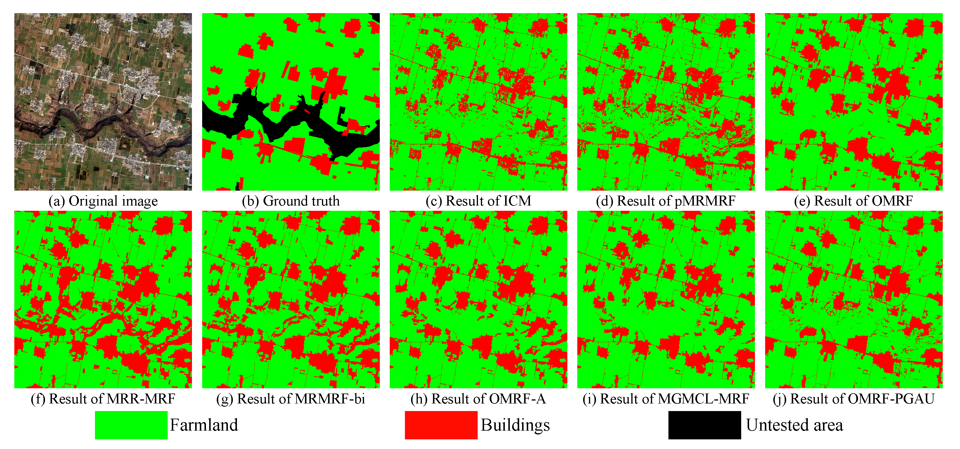
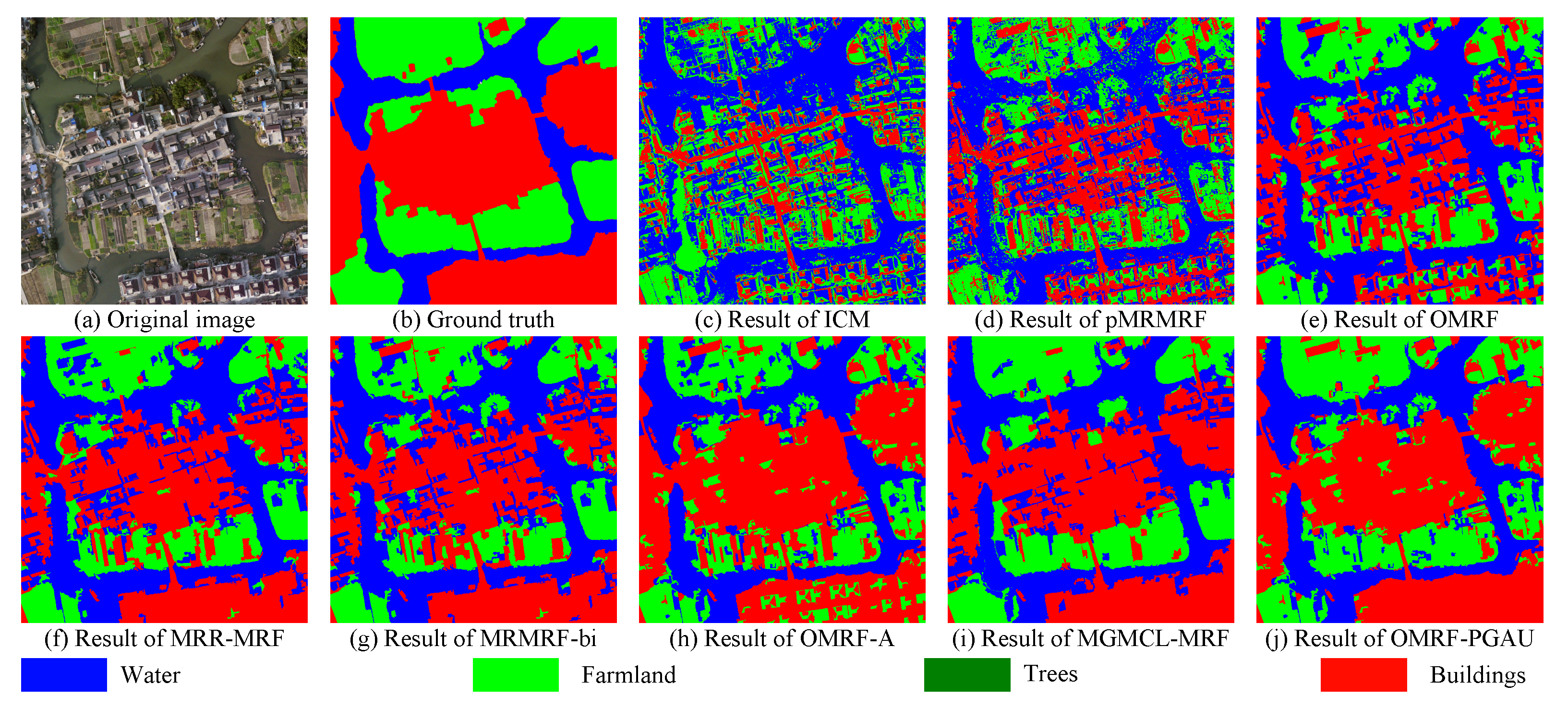
Figure 14	Kappa	0.5316	0.6152	0.6638	0.7758	0.7973	0.8480	0.8868	0.9018
	OA	0.6795	0.7466	0.7815	0.8740	0.9013	0.9266	0.9467	0.9607

.

For the Figure 12a, the RGB channel value of the buildings has a large variation range, and there are many shaded areas in the buildings part whose features are very similar to those of trees part. The features of the farmland part are also very close to the features of water part. These all bring challenges to semantic segmentation. Therefore, the results of ICM and pMRMRF are very poor. The OMRF, MRR-MRF, and MRMRF-bi all mistaken the farmland part into the water part, and mistaken the tree part in the upper-left part into the water part, but the division of the buildings part keeps the consistency of the area. OMRF-A distinguishes the cultivated land part mainly because of the auxiliary marker field, but for the tree part on the upper left of the image, there is still misclassification. Compared with OMRF-A, MGMCL-MRF has been improved. The upper left part of the tree is segmented and identified. This is because of the multi-granularity and multi-category concept, but in the lower right part, some areas are mistakenly classified as water. The segmentation result of OMRF-PGAU is the closest to reality. Both the farmland and the trees part on the upper-left are identified. In the lower half of the image, the trees part and the water part are also clearly distinguished. This is because in the segmentation process, the corresponding category number is set for the partition images, so that all objects in each partition image can be identified, and projected into the merged image to form an auxiliary label field and assist in the update of segmentation results in the subsequent update process.

For Figure 13a, the buildings are very sparsely distributed in the image. In the farmland, there are both green planted areas and yellow unplanted areas. There are paths connecting the buildings. However, due to the database labeling, the paths are classified as farmland. The pixel-level algorithms, ICM and pMRMRF, have a large number of misclassified pixels, and the edges of some buildings are swallowed by surrounding farmland. The segmentation effect of the object-level algorithms have been improved, but they are not ideal. Among them, MRR-MRF and MRMRF-bi divide many valley areas into building categories. OMRF-A and MGMCL-MRF can identify a large number of the buildings pixel, but some areas of farmland are misclassified. OMRF-PGAU has a relatively complete segmentation of buildings, but there are also misclassified areas in the farmland that appear to be salt and pepper. In contrast, the recognition accuracy of OMRF-PGAU is the highest.

For the Figure 14a, the farmland part in the image is also scattered with many small-scale building parts, which will affect the lower recognition in the segmentation. With the increase of image size, many block misclassification phenomena have also appeared in object-level methods. The segmentation results of ICM and pMRMRF are very poor, and OMRF also has many areas that are misclassified as water in the farmland part. The results of MRR-MRF and MRMRF-bi have a good completeness of the division for farmland part, and there is no large area of farmland that is mistakenly classified as water, but many farmlands are mistakenly classified as buildings. The result of OMRF-A still has many areas where farmland is mistakenly classified as water. The segmentation results of MGMCL-MRF and OMRF-PGAU are better, the three objects are identified better. OMRF-PGAU maintains a high regional consistency for the upper-left part of the buildings part, and the buildings part in the farmland part has not invaded to much of the farmland part.

3.4.4. Segmentation for Aerial Images

In Figure 15, Figure 16 and Figure 17, the near-ground aerial image taken in Taizhou is selected as the experimental image to further test the segmentation performance of the proposed method. The size of Figure 15a is 1024 × 1024, its spatial resolution is 0.4 m. The size of Figure 16a is 2240 × 2240, and the size of Figure 17a is 5000 × 5000, these two have the 0.1 m spatial resolution. These three aerial images contain three types of targets: buildings, farmland, and water. The increase in spatial resolution makes each type of object contain many sub-objects. For example, the farmland part includes both red roof, gray roof, white yard, and shaded parts. For the farmland part, it includes yellow land where no crops are planted, and green land where crops are planted. As for the water, some of the water has green algae and some of the water has a darker color. They are easily confused with farmland. The results of each segmentation method are shown in Figure 15, Figure 16 and Figure 17, and the segmentation accuracy indicators are shown in

Table 4. Quantitative indicators of eight comparison methods for three aerial images.

Methods		ICM	pMRMRF	OMRF	MRR-MRF	MRMRF-bi	OMRF-A	MGMCL-MRF	OMRF-PGAU
Figure 15	Kappa	0.6802	0.8123	0.8582	0.8489	0.8695	0.8811	0.9415	0.9490
	OA	0.7582	0.8656	0.9009	0.8939	0.9099	0.9190	0.9617	0.9670
Figure 16	Kappa	0.4230	0.5562	0.6239	0.7115	0.6976	0.7773	0.8124	0.8524
	OA	0.4786	0.6181	0.6859	0.7723	0.7598	0.8372	0.8621	0.8969
Figure 17	Kappa	0.4839	0.5450	0.6742	0.7305	0.7146	0.7803	0.7806	0.8359
	OA	0.5790	0.6415	0.7625	0.8135	0.8018	0.8661	0.8666	0.9067

.

For the Figure 15a, the three categories included in the image are more obvious, so the results of each segmentation algorithm are better. Pixel-level algorithms still have a large number of misclassified pixels. Among the object-level algorithms, OMRF, MRR-MRF, MRMRF-bi, and OMRF-A are not ideal for identifying contaminated water (that is, the middle left part of the figure), and part of the farmland is identified as a building at the bottom left. The farmland has not been planted without cultivated land. For the water in the middle part of the figure and the farmland segmentation at the bottom left, MGMCL-MRF and the algorithm proposed in this paper have the best results. The OMRF-PGAU result maintains good regional consistency of farmland. In contrast, the recognition accuracy of OMRF-PGAU is the highest.

It can be seen that the segmentation results of ICM and pMRMRF have many misclassified pixels, which makes the segmentation result form salt and pepper phenomenon, as shown in Figure 16c,d. The object-level segmentation method has been significantly improved, as shown in Figure 16e. MRR-MRF and MRMRF-bi misinterpret the dark shadows of some architectural areas as water, mainly because the RGB channel values of the two are very similar. OMRF-A has improved this phenomenon because the use of auxiliary label fields has improved the classification accuracy. MGMCL-MRF further confirms that each sub-object can be divided into a major object by combining multi-granularity and multi-class label fields. The proposed OMRF-PGAU assists the segmentation task by constructing partition images and merging images, and finally obtains more realistic segmentation labels.

As for the Figure 17a, the accuracies of pixel-level segmentation results are generally not high. The results of OMRF have been significantly improved, but a large amount of farmland has been mistakenly classified as water. MRR-MRF and MRMRF-bi maintain the regional consistency of the segmentation results because of the introduction of a multi-resolution structure. OMRF-A and MGMCL-MRF obtain higher segmentation results with the aid of multi-label fields. OMRF-APM uses partitioned images and a multi-granularity structure to fully excavate the information in the image using a circular path that alternately updates the total partitions. The segmentation result of OMRF-PGAU is the best among several methods.

3.5. Computational Time

The computational complexity of the OMRF-PGAU algorithm is of the same order of magnitude as OMRF, $O\left(\left[K^{\left(1\right)}·n\left(1\right)+K^{\left(2\right)}·n\left(2\right)+K^{\left(3\right)}·n\left(3\right)+K^{\left(4\right)}·n\left(4\right)+K·n\right]t\right)$, where $K^{\left(i\right)}$ is the number of the classes for $I^{\left(i\right)}$, $n\left(i\right)$ is a number of the vertexes for $I^{\left(i\right)}$, K is the number of the classes for I, n is a number of the vertexes for I, and t is the number of iterations. To further test the calculation speed of OMRF-PGAU, we counted the calculation time of all experiments in this paper, and the statistics are shown in

Table 5. The computational time of eight methods for the experimental images.

Time/s	ICM	pMRMRF	OMRF	MRR-MRF	MRMRF-bi	OMRF-A	MGMCL-MRF	OMRF-PGAU
Figure 6a	1.23	27.38	14.74 + 0.89	24.64 + 7.71	25.01 + 7.13	13.94 + 1.53	20.44 + 1.82	21.74 + 0.93
Figure 7a	2.31	27.94	15.11 + 0.91	24.69 + 7.44	25.33 + 6.32	14.21 + 1.90	20.53 + 1.79	20.38 + 0.99
Figure 8a	2.47	28.51	15.73 + 0.91	24.21 + 6.89	25.19 + 6.77	14.29 + 1.82	21.01 + 1.92	21.43 + 0.95
Figure 9a	0.98	14.64	10.86 + 0.45	20.98 + 5.65	21.27 + 5.82	11.30 + 1.14	19.48 + 0.99	19.93 + 1.12
Figure 10a	8.77	129.85	118.23 + 4.98	150.27 + 35.47	159.92 + 34.19	119.64 + 8.37	142.49 + 7.66	143.06 + 5.95
Figure 11a	13.64	195.05	121.34 + 5.16	148.33 + 38.62	151.63 + 39.14	120.03 + 8.26	138.41 + 8.33	137.05 + 6.02
Figure 12a	18.22	239.21	143.95 + 6.83	170.49 + 45.73	172.31 + 47.11	144.06 + 9.13	156.63 + 10.02	155.71 + 9.21
Figure 13a	22.47	362.07	180.34 + 8.24	217.87 + 61.46	219.19 + 59.30	178.54 + 11.54	204.05 + 11.95	200.12 + 10.52
Figure 14a	33.93	436.18	233.78 + 15.83	260.49 + 113.26	258.44 + 116.92	231.81 + 19.05	244.14 + 20.01	239.74 + 18.06
Figure 15a	10.84	138.27	101.32 + 4.16	132.93 + 31.59	129.04 + 32.93	100.74 + 6.28	120.58 + 7.26	117.50 + 6.34
Figure 16a	28.14	397.28	280.54 + 10.37	300.67 + 74.29	298.43 + 76.04	276.97 + 13.54	283.45 + 12.49	285.85 + 12.86
Figure 17a	43.92	430.41	430.69 + 25.47	450.43 + 150.03	423.51 + 137.31	403.93 + 37.51	585.18 + 30.48	614.82 + 29.31

.

It can be seen that all object-level algorithms need to initialize the over-segmented image, and for multi-layer structures, this stage takes a relatively long time. In subsequent update iterations, there are fewer good things about object-level algorithms than pixel-level algorithms. Among them, the time-consuming OMRF-PGAU algorithm proposed in this paper is at an average level.

4. Discussion

In the above chapters, the theoretical basis, update path, and segmentation performance of OMRF-PGAU are introduced in detail. The experimental chapter further verifies the superiority of OMRF-PGAU in semantic segmentation of remote sensing images. The advantages of OMRF-PGAU are mainly reflected in the following points: first, this method is an object-based segmentation method. Compared to the pixel-level segmentation method, it can consider a more macroscopic spatial neighborhood relationship, and the segmentation result can maintain a certain trend. Second, this method adopts a path of an alternate update of the entire partition, which can effectively avoid the segmentation result from falling into the local optimum. In the update process, the local update projection is used to project the global back to the local area, which not only ensures the independence of small regions, but also ensures the integrity of the large area. Third, this method combines the actual situation in different layers and sets different classification numbers for the partition and the whole, which can better classify the subclasses that have obviously different RGB channel values, but belong to the same category, into the same category. Finally, this method sets different regional granularity for the partition images and the original image, which reduces the misclassification caused by unreasonable intensity settings.

It should be noted that the algorithm OMRF-PGAU proposed in this paper contains many parameters that need to be statistically estimated or manually set, but the setting strategy of these parameters is given in Section 3.2, and it is explained that the algorithm is robust when the parameter setting is within a certain range. For example, the Gaussian distribution in the feature field needs to calculate the mean and covariance of the corresponding category based on the features and segmentation labels of each pixel. The unbiased estimation is used in this paper to calculate the parameter involved Gaussian distribution. Another example is the parameter setting of the energy function for the label field. This parameter is mainly used to adjust the influence of the feature field and the label field on the segmentation result. This paper sets the value range suitable for OMRF-PGAU through experiments.

5. Conclusions

In this paper, an object-level Markov random field method with partition-global alternately updated is proposed to realize the semantic segmentation of remote sensing images. The contribution of the high method is mainly reflected in two points: first, the method of alternate update of the partition as a whole was adopted. The original image was used to construct four partition images of the same size and a slightly smaller size, and form an auxiliary layer. Through the alternate update of the auxiliary layer and the original layer, the category that originally occupied a relatively small amount in the original image was not swallowed by other categories. Second, we used the correlation assumption to update the auxiliary layer and the original layer separately. Using the correlation assumption, the corresponding relationship between the auxiliary layer and the original layer was established, and it was applied to the update of the label field. The effectiveness of OMRF-PGAU was verified on different texture data and remote sensing image data in the experimental part. Compared with other selected MRF-based semantic segmentation comparison methods, the segmentation results of OMRF-PGAU proposed in this article have improved in both Kappa and OA, with an average improvement of 4% and a maximum improvement of 6%.

References

- Khare, S.; Latifi, H.; Khare, S. Vegetation Growth Analysis of UNESCO World Heritage Hyrcanian Forests Using Multi-Sensor Optical Remote Sensing Data. Remote Sens. 2021, 13, 3965. [Google Scholar] [CrossRef]
- Xia, J.; Luan, G.; Zhao, F.; Peng, Z.; Song, L.; Tan, S.; Zhao, Z. Exploring the Spatial–Temporal Analysis of Coastline Changes Using Place Name Information on Hainan Island, China. ISPRS Int. J.-Geo-Inf. 2021, 10, 609. [Google Scholar] [CrossRef]
- Phiri, D.; Morgenroth, J. Developments in Landsat Land Cover Classification Methods: A Review. Remote Sens. 2017, 9, 967. [Google Scholar] [CrossRef] [Green Version]
- Lyu, H.M.; Shen, J.S.; Arulrajah, A. Assessment of Geohazards and Preventative Countermeasures Using AHP Incorporated with GIS in Lanzhou, China. Sustainability 2018, 10, 304. [Google Scholar] [CrossRef] [Green Version]
- Ghamisi, P.; Maggiori, E.; Li, S.; Souza, R.; Tarablaka, Y.; Moser, G.; De Giorgi, A.; Fang, L.; Chen, Y.; Chi, M.; et al. New Frontiers in Spectral-Spatial Hyperspectral Image Classification: The Latest Advances Based on Mathematical Morphology, Markov Random Fields, Segmentation, Sparse Representation, and Deep Learning. IEEE Geosci. Remote Sens. Mag. 2018, 6, 10–43. [Google Scholar] [CrossRef]
- Zhong, Y.; Lin, X.; Zhang, L. A Support Vector Conditional Random Fields Classifier With a Mahalanobis Distance Boundary Constraint for High Spatial Resolution Remote Sensing Imagery. IEEE J. Sel. Top. Appl. Earth Obs. Remote Sens. 2014, 7, 1314–1330. [Google Scholar] [CrossRef]
- Zagajewski, B.; Kluczek, M.; Raczko, E.; Njegovec, A.; Dabija, A.; Kycko, M. Comparison of Random Forest, Support Vector Machines, and Neural Networks for Post-Disaster Forest Species Mapping of the Krkonoše/Karkonosze Transboundary Biosphere Reserve. Remote Sens. 2021, 13, 2581. [Google Scholar] [CrossRef]
- Lantzanakis, G.; Mitraka, Z.; Chrysoulakis, N. X-SVM: An Extension of C-SVM Algorithm for Classification of High-Resolution Satellite Imagery. IEEE Trans. Geosci. Remote Sens. 2021, 59, 3805–3815. [Google Scholar] [CrossRef]
- Peng, C.; Li, Y.; Jiao, L.; Chen, Y.; Shang, R. Densely Based Multi-Scale and Multi-Modal Fully Convolutional Networks for High-Resolution Remote-Sensing Image Semantic Segmentation. IEEE J. Sel. Top. Appl. Earth Obs. Remote Sens. 2019, 12, 2612–2626. [Google Scholar] [CrossRef]
- Pan, S.; Tao, Y.; Nie, C.; Chong, Y. PEGNet: Progressive Edge Guidance Network for Semantic Segmentation of Remote Sensing Images. IEEE Geosci. Remote Sens. Lett. 2021, 18, 637–641. [Google Scholar] [CrossRef]
- Tao, Y.; Xu, M.; Zhang, F.; Du, B.; Zhang, L. Unsupervised-Restricted Deconvolutional Neural Network for Very High Resolution Remote-Sensing Image Classification. IEEE Trans. Geosci. Remote Sens. 2017, 55, 6805–6823. [Google Scholar] [CrossRef]
- Hua, W.; Xie, W.; Jin, X. Three-Channel Convolutional Neural Network for Polarimetric SAR Images Classification. IEEE J. Sel. Top. Appl. Earth Obs. Remote Sens. 2020, 13, 4895–4907. [Google Scholar] [CrossRef]
- Wu, J.; Pan, Z.; Lei, B.; Hu, Y. LR-TSDet: Towards Tiny Ship Detection in Low-Resolution Remote Sensing Images. Remote Sens. 2021, 13, 3890. [Google Scholar] [CrossRef]
- Gray, P.C.; Chamorro, D.F.; Ridge, J.T.; Kerner, H.R.; Ury, E.A.; Johnston, D.W. Temporally Generalizable Land Cover Classification: A Recurrent Convolutional Neural Network Unveils Major Coastal Change through Time. Remote Sens. 2021, 13, 3953. [Google Scholar] [CrossRef]
- Dechesne, C.; Lassalle, P.; Lefèvre, S. Bayesian U-Net: Estimating Uncertainty in Semantic Segmentation of Earth Observation Images. Remote Sens. 2021, 13, 3836. [Google Scholar] [CrossRef]
- Wang, H.; Wang, Y.; Zhang, Q.; Xiang, S.; Pan, C. Gated Convolutional Neural Network for Semantic Segmentation in High-Resolution Images. Remote Sens. 2017, 9, 446. [Google Scholar] [CrossRef] [Green Version]
- Xu, Y.; Xie, Z.; Feng, Y.; Chen, Z. Road Extraction from High-Resolution Remote Sensing Imagery Using Deep Learning. Remote Sens. 2018, 10, 1461. [Google Scholar] [CrossRef] [Green Version]
- Bi, H.; Sun, J.; Xu, Z. A Graph-Based Semisupervised Deep Learning Model for PolSAR Image Classification. IEEE Trans. Geosci. Remote Sens. 2019, 57, 2116–2132. [Google Scholar] [CrossRef]
- Ding, L.; Zhang, J.; Bruzzone, L. Semantic Segmentation of Large-Size VHR Remote Sensing Images Using a Two-Stage Multiscale Training Architecture. IEEE Trans. Geosci. Remote Sens. 2020, 58, 5367–5376. [Google Scholar] [CrossRef]
- Zhan, T.; Gong, M.; Jiang, X.; Zhang, M. Unsupervised Scale-Driven Change Detection With Deep Spatial–Spectral Features for VHR Images. IEEE Trans. Geosci. Remote Sens. 2020, 58, 5653–5665. [Google Scholar] [CrossRef]
- Mboga, N.; D’Aronco, S.; Grippa, T.; Pelletier, C.; Georganos, S.; Vanhuysse, S.; Wolff, E.; Smets, B.; Dewitte, O.; Lennert, M.; et al. Domain Adaptation for Semantic Segmentation of Historical Panchromatic Orthomosaics in Central Africa. ISPRS Int. J.-Geo-Inf. 2021, 10, 523. [Google Scholar] [CrossRef]
- Daranagama, S.; Witayangkurn, A. Automatic Building Detection with Polygonizing and Attribute Extraction from High-Resolution Images. ISPRS Int. J.-Geo-Inf. 2021, 10, 606. [Google Scholar] [CrossRef]
- Feng, W.; Li, X.; Gao, G.; Chen, X.; Liu, Q. Multi-Scale Global Contrast CNN for Salient Object Detection. Sensors 2020, 20, 2656. [Google Scholar] [CrossRef]
- Zhu, L.; Gao, D.; Jia, T.; Zhang, J. Using Eco-Geographical Zoning Data and Crowdsourcing to Improve the Detection of Spurious Land Cover Changes. Remote Sens. 2021, 13, 3244. [Google Scholar] [CrossRef]
- Li, Z.; Zhang, Y. Hyperspectral Anomaly Detection via Image Super-Resolution Processing and Spatial Correlation. IEEE Trans. Geosci. Remote Sens. 2021, 59, 2307–2320. [Google Scholar] [CrossRef]
- Wei, Y.; Ji, S. Scribble-Based Weakly Supervised Deep Learning for Road Surface Extraction From Remote Sensing Images. IEEE Trans. Geosci. Remote Sens. 2022, 60, 816–820. [Google Scholar] [CrossRef]
- Besag, J. On the Statistical-Analysis of Dirty Pictures. J. R. Stat. Soc. 1986, B-48, 259–302. [Google Scholar] [CrossRef] [Green Version]
- Zheng, C.; Wang, L.; Chen, R.; Chen, X. Image Segmentation Using Multiregion-Resolution MRF Model. IEEE Geosci. Remote Sens. Lett. 2013, 10, 816–820. [Google Scholar] [CrossRef]
- Zheng, C.; Zhang, Y.; Wang, L. Semantic Segmentation of Remote Sensing Imagery Using an Object-Based Markov Random Field Model With Auxiliary Label Fields. IEEE Trans. Geosci. Remote Sens. 2017, 55, 3015–3028. [Google Scholar] [CrossRef]
- Zheng, C.; Wang, L.; Chen, X. A Hybrid Markov Random Field Model With Multi-Granularity Information for Semantic Segmentation of Remote Sensing Imagery. IEEE J. Sel. Top. Appl. Earth Obs. Remote Sens. 2019, 12, 2728–2740. [Google Scholar] [CrossRef]
- Zheng, C.; Yao, H. Segmentation for remote-sensing imagery using the object-based Gaussian-Markov random field model with region coefficients. Int. J. Remote Sens. 2019, 40, 4441–4472. [Google Scholar] [CrossRef]
- Zheng, C.; Zhang, Y.; Wang, L. Multigranularity Multiclass-Layer Markov Random Field Model for Semantic Segmentation of Remote Sensing Images. IEEE Trans. Geosci. Remote Sens. 2020, 59, 10555–10574. [Google Scholar] [CrossRef]
- Zheng, C.; Chen, Y.; Shao, J.; Wang, L. An MRF-Based Multigranularity Edge-Preservation Optimization for Semantic Segmentation of Remote Sensing Images. IEEE Geosci. Remote Sens. Lett. 2021, 1–5. [Google Scholar] [CrossRef]
- Li, X.; Chen, J.; Zhao, L.; Guo, S.; Sun, L.; Zhao, X. Adaptive Distance-Weighted Voronoi Tessellation for Remote Sensing Image Segmentation. Remote Sens. 2020, 12, 4115. [Google Scholar] [CrossRef]
- Skurikhin, A.N. Hidden Conditional Random Fields for land-use classification. In Proceedings of the 2015 IEEE International Geoscience and Remote Sensing Symposium (IGARSS), Milan, Italy, 26–31 July 2015; pp. 4376–4379. [Google Scholar] [CrossRef]
- Wang, F.; Wu, Y.; Li, M.; Zhang, P.; Zhang, Q. Adaptive Hybrid Conditional Random Field Model for SAR Image Segmentation. IEEE Trans. Geosci. Remote Sens. 2017, 55, 537–550. [Google Scholar] [CrossRef]
- Feng, W.; Sui, H.; Huang, W.; Xu, C.; An, K. Water Body Extraction From Very High-Resolution Remote Sensing Imagery Using Deep U-Net and a Superpixel-Based Conditional Random Field Model. IEEE Geosci. Remote Sens. Lett. 2019, 16, 618–622. [Google Scholar] [CrossRef]
- Nagi, A.S.; Kumar, D.; Sola, D.; Scott, K.A. RUF: Effective Sea Ice Floe Segmentation Using End-to-End RES-UNET-CRF with Dual Loss. Remote Sens. 2021, 13, 2460. [Google Scholar] [CrossRef]
- Cheng, J.; Zhang, F.; Xiang, D.; Yin, Q.; Zhou, Y.; Wang, W. PolSAR Image Land Cover Classification Based on Hierarchical Capsule Network. Remote Sens. 2021, 13, 3132. [Google Scholar] [CrossRef]
- Osher, S.; Sethian, J.A. Fronts propagating with curvature-dependent speed: Algorithms based on Hamilton-Jacobi formulations. J. Comput. Phys. 1988, 79, 12–49. [Google Scholar] [CrossRef] [Green Version]
- Ball, J.E.; Bruce, L.M. Level Set Hyperspectral Image Classification Using Best Band Analysis. IEEE Trans. Geosci. Remote Sens. 2007, 45, 3022–3027. [Google Scholar] [CrossRef]
- Li, Z.; Shi, W.; Myint, S.W.; Lu, P.; Wang, Q. Semi-automated landslide inventory mapping from bitemporal aerial photographs using change detection and level set method. Remote Sens. Environ. 2016, 175, 215–230. [Google Scholar] [CrossRef]
- Noda, H.; Shirazi, M.N.; Kawaguchi, E. MRF-based texture segmentation using wavelet decomposed images. Pattern Recognit. 2002, 35, 771–782. [Google Scholar] [CrossRef] [Green Version]
- Yao, H.; Zhang, M.; Wang, B. A Top-Down Application of Multi-Resolution Markov Random Fields with Bilateral Information in Semantic Segmentation of Remote Sensing Images. In Proceedings of the 2018 26th International Conference on Geoinformatics, Kunming, China, 28–30 June 2018; pp. 1–6. [Google Scholar] [CrossRef]
- Hossain, M.D.; Chen, D. Segmentation for Object-Based Image Analysis (OBIA): A review of algorithms and challenges from remote sensing perspective. ISPRS J. Photogramm. Remote Sens. 2019, 150, 115–134. [Google Scholar] [CrossRef]
- Xia, G.s.; He, C.; Sun, H. An Unsupervised Segmentation Method Using Markov Random Field on Region Adjacency Graph for SAR Images. In Proceedings of the 2006 CIE International Conference on Radar, Shanghai, China, 16–19 October 2006; pp. 1–4. [Google Scholar] [CrossRef]
- Besag, J. Spatial Interaction and the Statistical Analysis of Lattice Systems. J. R. Stat. Soc. Ser. (Methodol.) 1974, 36, 192–225. [Google Scholar] [CrossRef]
- Comaniciu, D.; Meer, P. Mean shift: A robust approach toward feature space analysis. IEEE Trans. Pattern Anal. Mach. Intell. 2002, 24, 603–619. [Google Scholar] [CrossRef] [Green Version]
- Mikes, S.; Haindl, M. Texture Segmentation Benchmark. IEEE Trans. Pattern Anal. Mach. Intell. 2021, 1. [Google Scholar] [CrossRef]
- Tong, X.Y.; Xia, G.S.; Lu, Q.; Shen, H.; Li, S.; You, S.; Zhang, L. Land-cover classification with high-resolution remote sensing images using transferable deep models. Remote Sens. Environ. 2020, 237, 111322. [Google Scholar] [CrossRef] [Green Version]
- Unnikrishnan, R.; Hebert, M. Measures of Similarity. In Proceedings of the 2005 Seventh IEEE Workshops on Applications of Computer Vision (WACV/MOTION’05)—Volume 1, Breckenridge, CO, USA, 5–7 January 2005; Volume 1, p. 394. [Google Scholar] [CrossRef]