Article

Improved Method to Detect the Tailings Ponds from Multispectral Remote Sensing Images Based on Faster R-CNN and Transfer Learning

1
Aerospace Information Research Institute, Chinese Academy of Sciences, Beijing 100094, China
2
School of Electronic, Electrical and Communication Engineering, University of Chinese Academy of Sciences, Beijing 100049, China
3
Institute of Mineral Resources Research, China Metallurgical Geology Bureau, Beijing 101300, China
4
Key Laboratory of Earth Observation of Hainan Province, Hainan Research Institute, Aerospace Information Research Institute, Chinese Academy of Sciences, Sanya 572000, China
*
Author to whom correspondence should be addressed.
Remote Sens. 2022, 14(1), 103; https://doi.org/10.3390/rs14010103
Submission received: 13 November 2021 / Revised: 16 December 2021 / Accepted: 22 December 2021 / Published: 26 December 2021
(This article belongs to the Special Issue Environmental Health Diagnosis Based on Remote Sensing)

Abstract

:
The breaching of tailings pond dams may lead to casualties and environmental pollution; therefore, timely and accurate monitoring is an essential aspect of managing such structures and preventing accidents. Remote sensing technology is suitable for the regular extraction and monitoring of tailings pond information. However, traditional remote sensing is inefficient and unsuitable for the frequent extraction of large volumes of highly precise information. Object detection, based on deep learning, provides a solution to this problem. Most remote sensing imagery applications for tailings pond object detection using deep learning are based on computer vision, utilizing the true-color triple-band data of high spatial resolution imagery for information extraction. The advantage of remote sensing image data is their greater number of spectral bands (more than three), providing more abundant spectral information. There is a lack of research on fully harnessing multispectral band information to improve the detection precision of tailings ponds. Accordingly, using a sample dataset of tailings pond satellite images from the Gaofen-1 high-resolution Earth observation satellite, we improved the Faster R-CNN deep learning object detection model by increasing the inputs from three true-color bands to four multispectral bands. Moreover, we used the attention mechanism to recalibrate the input contributions. Subsequently, we used a step-by-step transfer learning method to improve and gradually train our model. The improved model could fully utilize the near-infrared (NIR) band information of the images to improve the precision of tailings pond detection. Compared with that of the three true-color band input models, the tailings pond detection average precision (AP) and recall notably improved in our model, with the AP increasing from 82.3% to 85.9% and recall increasing from 65.4% to 71.9%. This research could serve as a reference for using multispectral band information from remote sensing images in the construction and application of deep learning models.

Graphical Abstract

1. Introduction

Tailings ponds house tailings after mining and beneficiation. The term usually refers to a place to store metal and non-metal tailings or other industrial waste after ore separation, with a dam enclosing such a site constructed across a valley mouth or on flat terrain [1]. Because of the complex composition of tailings ponds, their constituent tailings and tailing water usually contain harmful elements. Consequently, leakages or dam breaks have grave consequences for downstream residents and the environment [2]. In recent years, frequent environmental disasters have been caused by tailings pond failures, resulting in numerous casualties and severe environmental pollution [3]. It is imperative, therefore, to improve the investigation and governance of mining conditions during development and, particularly, the monitoring and management of mine tailings ponds [4].
As remote sensing is dynamic, almost unconstrained by ground conditions, and able to cover large areas, it has become an important monitoring method for environmental protection [5,6]. Numerous tailings ponds exist, usually located in remote mountains and valleys, and using remote sensing technology to identify and monitor them overcomes the problems associated with traditional ground surveys, such as them being time-consuming and laborious, and having poor precision. For example, Fu et al. [7] extracted the environmental information of a mine tailings pond area in western Sichuan from multi-temporal high-resolution remote sensing imagery obtained from a Chinese satellite and monitored changes to analyze potential dangers. Zhou et al. [4] used high-resolution remote sensing imagery to conduct remote sensing interpretation, identifying the types, number, location, size, and uses of tailings ponds in Shandong Province, China. Zhao [8] conducted remote sensing monitoring research of the tailings ponds at Taershan in Shanxi Province, extracting information on the number, area, and constituent minerals of these tailings ponds.
Traditional remote sensing has played a key role in extracting and monitoring tailings pond information, but persistent issues, including the inability to handle large workloads and low automation and intelligence, have made it unsuitable for large-scale, high-frequency information extraction and monitoring within a big data context. Object detection, based on the rapidly developing field of deep learning, has made significant progress in terms of precision, effectiveness, and automation as an end-to-end model compared with traditional object detection methods [9]. Consequently, the application of object detection in remote sensing has become a growing area of interest. Bai et al. [10] have introduced an improved Faster R-CNN model [11] that uses the dense residual network to improve feature extraction and solve region mismatch problems. As such, the precision of automatic building detection from high-resolution UAV remote sensing imagery is improved. Zambanini et al. [12] have also used Faster R-CNN, together with images from the WorldView-3 high spatial resolution Earth imaging satellite to automatically detect parked vehicles in an urban area. Wang et al. [13] used transfer learning to improve the Mask R-CNN model [14], constructed an open-pit mine detection model using high-resolution remote sensing data, and achieved automatic identification and dynamic monitoring of open-pit mines. Machefer et al. [15] adjusted the hyperparameters of Mask R-CNN to achieve the automatic detection and segmentation of individual plants based on high-resolution UAV remote sensing imagery. Zhao et al. [16] have presented a method combining Mask R-CNN with building boundary regularization to generate more boundaries that are more accurate.
As regards tailings pond detection, Li et al. [17] have used a deep learning object detection model, the single shot multibox detector (SSD) [18] to extract the location of tailings ponds in the Beijing–Tianjin–Hebei region of China and to analyze their geographical distribution. These authors have proven that the deep learning method effectively detects features from remote sensing images. Compared with traditional methods, this method significantly improves the automation and effectiveness of tailings pond identification. Lyu et al. [19] proposed a framework for extracting tailings ponds that combines the object detection algorithm “you only look once” (YOLO) v4 [20] and the random forest algorithm. After extracting tailings ponds in the target area using the optimal random forest model, these authors used morphological processing to obtain the final extraction results. Their method could be used to extract the boundaries of tailing ponds in large areas. Yan et al. [21] developed an improved SSD model that increases extraction precision for large tailings ponds by adding convolutional layers. Zhang et al. [22] proposed an instance segmentation network with a multi-task branching structure which effectively improves tailings pond recognition precision. In a previous study [23], we proposed an improved Faster R-CNN by selecting the optimal model input size, strengthening the attention mechanism, and improving the feature pyramid network. These factors significantly improved the detection precision and effectiveness for tailings pond targets of high-resolution remote sensing images.
To summarize, most remote sensing imagery applications for tailings pond object detection using deep learning are based on computer vision, utilizing the true-color triple-band data of high spatial resolution imagery for information extraction. However, the advantage of remote sensing image data is their greater number of spectral bands (more than three), providing more abundant spectral information. In a previous study [23], we proposed an improved Faster R-CNN model based on the three true-color bands in high-resolution remote sensing data to improve the detection precision of tailings ponds. Therefore, in this study, we proposed an improved method based on Faster R-CNN and transfer learning to detect the tailings ponds from the Gaofen-1 (GF-1) satellite images, which have four multispectral bands. The experimental results showed that the proposed method could utilize the near-infrared (NIR) band in GF-1 images and exploit the rich spectral information of GF-1 images to significantly improve the precision of tailings pond detection.

2. Materials and Methods

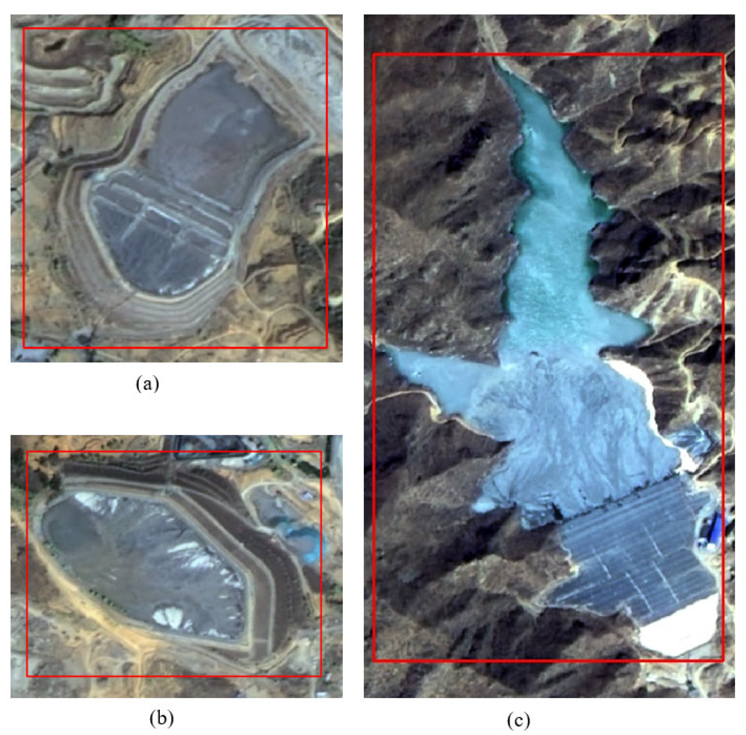
2.1. Data and Preprocessing

The GF-1 satellite, which launched on 26 April 2013, is China’s first high-resolution Earth observation satellite. The satellite is equipped with two 2 m panchromatic/8 m multispectral cameras and four 16 m multispectral cameras. In this study, we used the data from the 2 m panchromatic/8 m multispectral cameras to study tailings pond object detection. The specific index parameters are shown in Table 1 [17].
The acquired data derive from the L1A processing level. The data required preprocessing, including radiometric calibration, orthorectification, and image fusion. First, we performed radiometric calibration on the original data. Subsequently, to eliminate image geometric distortion and improve geometric accuracy, based on the rational polynomial coefficients file of the image and the digital elevation model data of the corresponding area, we performed orthorectification. Finally, we performed image fusion processing on the Pan band data and the blue, green, red, and NIR multispectral band data to generate multispectral image data with a spatial resolution of 2 m and containing four bands. These data were used as the tailings pond sample dataset.

2.2. Sampling Data Generation

We selected Hebei Province in China as the research area because of its substantial number of tailings ponds. Based on the GF-1 image data for this area, a total of 963 tailings pond samples were manually identified. The geographical distribution of the selected tailings pond samples is shown in Figure 1.
The shape of a tailings pond depends on the natural landscape as well as artificial and engineering features [24]. Tailings ponds could be divided into four types based on a range of factors, such as their topography and geomorphology, the resource being mined, the mining technology employed, and the scale of operations—namely cross-valley type, hillside type, stockpile type, and cross-river type [17]. Cross-valley type tailings ponds refer to those formed by building a dam at the mouth of a valley. The main characteristics are that the initial dam is relatively short, and the reservoir area is long and deep. Hillside-type tailings ponds refer to those surrounded by a dam body built at the foot of a hill. The main characteristics of these tailings ponds are that the initial dam is relatively long, and the depth of the reservoir area is short. Stockpile type tailings ponds are formed by building a dam around materials on a gently sloping area. Such tailings ponds require significant work to create the initial dam as well as to subsequently fill the dam, and these dams are generally not very high. Cross-river type tailings ponds are formed by damming the upper and lower reaches of rivers. Their primary feature is a large upstream catchment area and a complex tailings pond and upstream drainage system [23]. Cross-river tailings ponds are rarely found in Hebei Province, and the tailings pond sample in this study does not include any of this type, i.e., it only includes cross-valley type, hillside type, and stockpile type tailings ponds. Annotated GF-1 true-color fused images showing the features of the various types of tailings ponds are shown in Figure 2.
This study identified a total of 963 tailings ponds, 80% of which were used as the training sample set, and 20% were used as the test sample set. Before imputing the GF-1 image data, slicing had to be performed. To maximally ensure the integrity of tailings ponds in the sample slices, and given the limitations of computing hardware, such as graphics processing unit memory, we set the sample slice size to 1024 × 1024 pixels during slicing. The degree of overlap between the slices was set to 128 pixels to expand the characteristics of tailings ponds and increase the number of sample slices. The GF-1 image data are 16 bit, and the data conversion to 8 bits was performed on the sample slices. After the above processing and the filtering of invalid slices, we obtained a tailings pond sample dataset of GF-1 images. The detailed information of the dataset is shown in Table 2.

2.3. Methodology

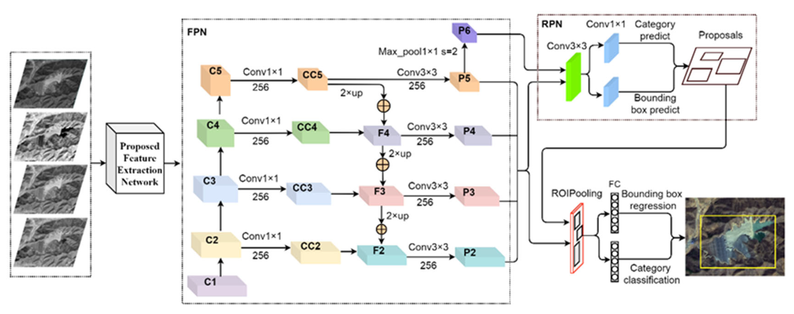
2.3.1. Proposed Method

In the field of computer vision, Faster R-CNN is a classic object detection model based on deep learning. The model has high recognition accuracy and efficiency when applied to large target areas and has been widely used for object detection from remote sensing images [10,12,23]. In this study, we introduced an improved Faster R-CNN model to make full use of the multispectral band information of GF-1 images and improve the precision of tailings pond detection, based on the research results in [23]. The structure of our model is shown in Figure 3.
(1)
The model inputs are the four spectral bands of GF-1 image data, namely blue, green, red, and NIR. After being passed through the proposed feature extraction network, the model outputs are multi-layer features (C1, C2, C3, C4, and C5).
(2)
The feature pyramid network (FPN) fuses shallow features and deep features using the semantic information of deep features and the location information of shallow features to further improve the performance of the network [25]. The multi-layer features C2, C3, C4, and C5 are the FPN inputs for feature merging, for which the number of channels are 256, 512, 1024, and 2048, respectively. First, through the 1 × 1 convolution operation (Conv1 × 1), C2, C3, C4, and C5 were subjected to dimensionality reduction, with the corresponding outputs CC2, CC3, CC4, and CC5, and the number of channels for each output was set to 256. Using the nearest neighbor difference method, CC5, CC4, and CC3 were up-sampled twice (2× up), and element-wise addition ( Remotesensing 14 00103 i001) was performed on CC4, CC3, and CC2 to merge the features of different layers, with the corresponding outputs F2, F3, and F4 (256 channels). A 3 × 3 convolution (Conv3 × 3) was conducted on F2, F3, and F4, generating P2, P3, and P4 (256 channels), and Conv3x3 was conducted on CC5, generating P5 (256 channel output). The maximum pooling was conducted on P5 of 1 × 1 with a stride of 2 (Max_pool 1 × 1 s = 2) and output P6 (256 channels). Features merging was completed with FPN, with the final set of feature maps being called {P2, P3, P4, P5, and P6}.
(3)
The multi-scale feature maps {P2, P3, P4, P5, and P6} were sent to the region proposal network (RPN), with the anchor areas set to {322, 642, 1282, 2562, and 5122} pixels, and the aspect ratios of the anchors set to {1:2, 1:1, and 2:1} to generate region proposals.
(4)
The region proposals needed to slice the region proposal feature maps from {P2, P3, P4, and P5}, and the following formula were used to select the most appropriate scale:
k   = k 0   + log 2 ( w h / H )
where k is the feature map layer corresponding to the region proposal, which is rounded during the calculation; k0 is the highest layer of the feature maps and, as there are four layers of feature maps in this study, we set k0 to 4; w and h represent the width and height of the region proposal, respectively; and H is the height and width of the model input. After the proposal, the feature maps were subjected to ROI pooling, and were sent to the subsequent fully connected (FC) layer to determine the object category and obtain the precise position of the bounding box. Based on the research results of [23], we improved the two following aspects:
(1)
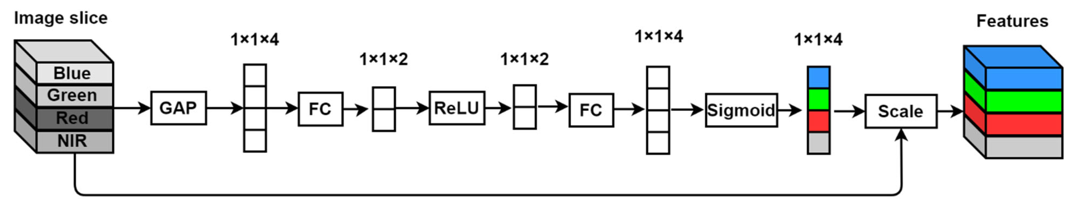
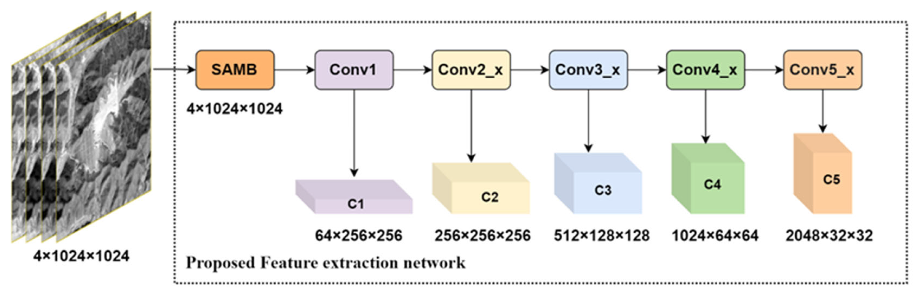
The feature extraction network was improved. The number of input channels was increased from three to four, which is the number of bands in GF-1 images. Unlike most studies that use the attention mechanism to recalibrate the contribution of the extracted feature channels, we used the attention mechanism to recalibrate the contribution of the original four bands. Details of our methodology are presented in the “Proposed feature extraction network” section below.
(2)
A step-by-step transfer learning method was adopted to gradually improve and train the model, of which details are presented in the “transfer learning” section below.

2.3.2. Proposed Feature Extraction Network

In recent years, the attention mechanism has been widely used in the field of deep learning to improve performance, and it has become an important concept in neural network models [26]. Essentially, the attention mechanism mimics the human brain by devoting more attention resources to the object area (i.e., the focus) to obtain information that is more detailed, while suppressing information from non-important areas. Mnih et al. [27] used the attention mechanism in a recurrent neural network model to improve the performance of the model image classification. Bahdanau et al. [28] used the attention mechanism in the field of natural language processing on a machine translation task to simultaneously translate and align. In the feature layer of the convolutional neural network, each channel represents a different feature, and these features differ in importance and in their contribution to the network performance. In object detection based on deep learning for remote sensing images, Li et al. [29] used the attention mechanism and Mask R-CNN, a convolutional neural network, to design an improved top–down FPN, which improved the detection precision of small objects with complex backgrounds for remote sensing images. Based on the YOLO network model [30], Hu et al. [31] proposed a more advanced small marine vessel object detection method using the attention mechanism of spatial and channel information. Squeeze-and-excitation networks [32] are based on the principle of the attention mechanism, automatically obtaining the importance of each feature channel. Based on this importance, features with a large contribution are promoted and features with a small contribution are suppressed, thereby improving the performance of image classification.
Rather than recalibrating the contribution of the extracted feature channels, our study designed an attention mechanism module for GF-1 image slices and recalibrated the contribution of the four bands of the input. With the addition of a few parameters and calculations, we significantly improved the detection precision for tailings ponds. The structure of the module is shown in Figure 4.
Image slice refers to the multi-band (blue, green, red, and NIR bands) data of GF-1 images. The slice size is 1024 × 1024 pixels, and the tensor size is 1024 × 1024 × 4. After applying global average pooling (GAP), the input tensor was compressed into a 1 × 1 × 4 one-dimensional vector. Each value in the vector has a global receptive field, representing the global distribution of responses on corresponding input bands. An FC layer was used for compression into a 1 × 1 × 2 one-dimensional vector. After applying the Relu activation function, the second FC layer restored the number of channels to four, producing a 1 × 1 × 4 one-dimensional vector. The sigmoid function was used subsequently to obtain normalized weights, resulting in a 1 × 1 × 4 one-dimensional vector, with each value in the vector representing the contribution of the corresponding input bands. Finally, using the scale, once the contribution weight of each band was extended to a dimension equal to its corresponding band, it was multiplied by the input band to obtain the features, which were used as the input features in the subsequent feature extraction network.
The proposed feature extraction network in this study comprised the slice attention mechanism block (SAMB) and five convolution blocks of ResNet-101 [33]—the structure is shown in Figure 5. The four multispectral bands of the image slice served as the input of the model. After the contribution of each band was recalibrated using the SAMB, the output of the SAMB was sent to the subsequent network, where Conv1, Conv2_x, Conv3_x, Conv4_x, and Conv5_x represented the five convolution blocks of ResNet-101. In the network, the number of channels of the Conv1 convolution kernel was expanded from three to four, the size and number of feature output channels remained unchanged, and the structure of the remaining convolution blocks remained unchanged. Each convolution block corresponds to the output features at different layers (C1, C2, C3, C4, and C5). In the case of C1, 64 × 256 × 256 means that the number of channels is 64 and the size is 256 × 256 pixels (the channels and sizes of the other layers are determined in a similar fashion). Layers C2, C3, C4, and C5 were used as input for subsequent FPN.

2.3.3. Transfer Learning

Insufficient training samples and computing power are commonly encountered problems during machine learning tasks. In recent years, transfer learning has emerged as an important technique for overcoming these issues. The essence of transfer learning is the transfer and reuse of knowledge [13]. Transfer learning consists of two elements, namely domains and tasks [34]. Domains are the main body of learning and contain two elements, which are the sample feature space Ӽ and the probability distribution P(X), where X = (x1, x2, …, xn) ∈ Ӽ. Given a specific domain, D = {Ӽ, P(X)}, a task T consists of two parts, namely a label space Y = (y1, y2, …, yn) and an objective predictive function f. The task consists of {xi, yi}, where xi ∈ X and yi ∈ Y and the target predictive function f are used to predict the corresponding label f(x) of a new sample x. From the perspective of probability, f(x) could be considered the conditional probability P(y|x), and task T could be expressed as T = {Y, p(y|x)}. Given a source domain Ds and learning task Ts, a target domain Dt and learning task Tt, where Ds ≠ Dt or Ts ≠ Tt, transfer learning aims to use the knowledge of Ds and Ts to improve the learning of the predictive function fT in the target domain Dt [35].
Transfer learning methods could be divided into four types, namely instance transfer, feature representation transfer, parameter transfer, and relational knowledge transfer [36]. Instance transfer assumes that parts of the data in the source domain could be reused in the target domain by reweighting. Feature representation transfer uses a good feature representation to reduce the difference between the source domain and the target domain and model errors. Relational knowledge transfer involves the mapping of relevant knowledge between the source domain and the target domain. The parameter transfer approach refers to the sharing of model parameters and prior knowledge between the source domain and the target domain, which is a quite commonly used transfer learning method in the field of deep learning.
Yosinski et al. [36] investigated the transferability of features in deep neural networks. The results of their study showed that using the fine-tuning transfer learning method with a trained deep neural network and parameters, fine-tuning parameters in a new task could better overcome the differences in data, improving the training efficiency and performance of the model.
The limited number of GF-1 tailings pond samples could lead to overfitting and as we intended, using multispectral band information to improve the tailings pond detection precision, we adopted a step-by-step transfer learning method to gradually improve and train the model. In the transfer learning method of our initial research, an ImageNet dataset was used as the source domain and the GF-1 four-band sample dataset was used as the target domain. The five convolution blocks (Conv1, Conv2_x, Conv3_x, Conv4_x, and Conv5_x) of the source domain pre-trained ResNet-101 were used as the feature extraction network of the target model. The number of band inputs was improved from three to four. The number of channels of the convolution kernel Conv1 improved from three to four, whereas the size and number of feature output channels remained unchanged. The first three channels of the convolution kernel Conv1 were initialized with pre-trained parameters, and the new fourth channel was initialized with the pre-trained third channel parameters. The rest of the feature extraction network was initialized with pre-trained parameters. The target model was trained and tested based on the target domain. The target model was named Bands_4. Our results showed that although the Bands_4 model included the additional NIR band information, the tailings pond detection precision of the model did not significantly improve.
To address this failure, we adopted a step-by-step transfer learning method to gradually improve and train the model. Only the feature extraction network was improved, whereas the other parts of the model remained unchanged. The process was as follows:
(1) An ImageNet dataset was used as the source domain, and a GF-1 true-color sample dataset (only the three true-color bands of the GF-1 sample data) was used as the target domain. The five convolution blocks (Conv1, Conv2_x, Conv3_x, Conv4_x, and Conv5_x) of the source domain pre-training ResNet-101 were used as the feature extraction network of the target model, and initialization was conducted with pre-trained parameters. The training and testing of the target model were completed based on the target domain. The target model in this step was named Bands_3.
(2) The GF-1 true-color sample dataset was used as the source domain, and the GF-1 four-band sample dataset was used as the target domain. The number of input bands of the feature extraction network of the source domain pre-trained model Bands_3 was improved by increasing the bands from three to four. The number of channels of the convolution kernel Conv1 was also improved from three to four, but the size and number of feature output channels was unchanged, and served as the feature extraction network of the target model. In the feature extraction network of the target model, the newly added fourth channel of Conv1 was initialized with pre-trained third channel parameters, and the rest was initialized with corresponding pre-trained parameters. We compared the use of pre-trained third channel parameters, second channel parameters, first channel parameters, and the average of the three channel parameters to initialize the newly added fourth channel of Conv1, that using the third channel parameters has the highest precision. The training and testing of the target model were completed based on the target domain. The target model in this step was named Bands_4_sub.
(3) The GF-1 four-band sample dataset was used as both the source domain and the target domain. We transferred the feature extraction network and parameters of the pre-trained Bands4_sub model and added a SAMB module to improve it, which served as the feature extraction network of the target model. The training and testing of the target model were completed based on the target domain. The target model in this step was named Bands4_sub_SAMB.
During our research, Kaiming normal initialization was used for model parameters (include SAMB), except for the feature extraction network, for which we used pre-trained model parameters. The steps of the transfer learning process are shown in Figure 6.

2.3.4. Accuracy Assessment

When evaluating the target detection results, the ground truth bounding box (GT) is the true bounding box of the predicted target, whereas the predicted bounding box (PT) is the predicted bounding box of the predicted target. The area encompassed by both the predicted bounding box and the ground truth is denoted as the area of union, the intersection is denoted as the area of overlap, and the calculation formula of the intersection over union (IOU) is as follows:
IOU = Area   of   Overlap Area   of   Union
where TP (true positive) refers to the number of detection boxes with correct detection results and an IOU > 0.5; false positive (FP) refers to the number of detection boxes with incorrect detection results and an IOU ≤ 0.5; and false negative (FN) refers to the number of GTs that are not detected. The model evaluation indicators used in this study were precision and recall. Precision refers to the ratio of the number of correct detection boxes to the total number of detection boxes, whereas recall refers to the ratio of the number of correct detection boxes to the total number of true bounding boxes. Their corresponding calculation formulas are as follows:
P r e c i s i o n = T P T P + F P
R e c a l l = T P T P + F N
The average precision (AP) of the target, precision–recall curve (PRC), and mean average precision (mAP) are three common indicators widely applied to evaluate the performance of object detection methods. AP is typically the area under the PRC and mAP is the average value of AP values for all classes; the larger the mAP value, the better the object detection performance. As this study only detects one target, namely a tailings pond, AP was used as the main model evaluation indicator, with the recall and time consumption of a single iteration used as reference indicators [23].

2.3.5. Loss Function

In this study, we used the loss function of Faster R-CNN, and the formula for the calculation can be expressed as follows [11]:
L ( p i , t i ) = 1 N c l s i L c l s ( p i , p i * ) + α 1 N r e g i p i * L r e g ( t i , t i * )
where Ncls represents the number of anchors in the mini batch, Nreg represents the number of anchor locations, and α represents the weight balance parameter, which was set to 10 in this study, and i represents the index of an anchor in a mini batch.
Furthermore, p i represents the predictive classification probability of the anchor. Specifically, when the anchor was positive, p i * = 1, and when it was negative, p i * = 0. Moreover, anchors that met the following two conditions were considered positive: (1) the anchor has the highest intersection-over-union (IOU) overlap with a ground truth box; or (2) the IOU overlap of the anchor with the ground truth box is >0.7. Conversely, when the IOU overlap of the anchor with any ground-truth box was <0.3, the anchor was considered negative. Anchors that were neither positive nor negative were not included in the training:
L c l s ( p i , p i * ) = log [ p i p i * + ( 1 p i ) ( 1 p i * ) ]
L r e g ( t i , t i * ) = i { x , y , w , h } S m o o t h L 1 ( t i t i * )
S m o o t h L 1 ( x ) = { 0.5 x 2 ,   i f | x | < 1 | x | 0.5 ,   o t h e r w i s e
For the bounding box regression, we adopted the parameterization of four coordinates, defined as follows:
t x = ( x x a ) w a ,   t y = ( y y a ) h a t w = log ( w w a ) ,   t h = log ( h h a ) t x * = ( x * x a ) w a ,   t y * = ( y * y a ) h a t w * = log ( w * w a ) ,   t h * = log ( h * h a )
where x and y represent the coordinates of the center of the bounding box, and w and h represent the width and height of the bounding box, respectively. Furthermore, x, xa, and x* correspond to the predicted box, anchor box, and ground truth box, respectively, similarly to y, w, and h.

2.3.6. Training Environment and Optimization
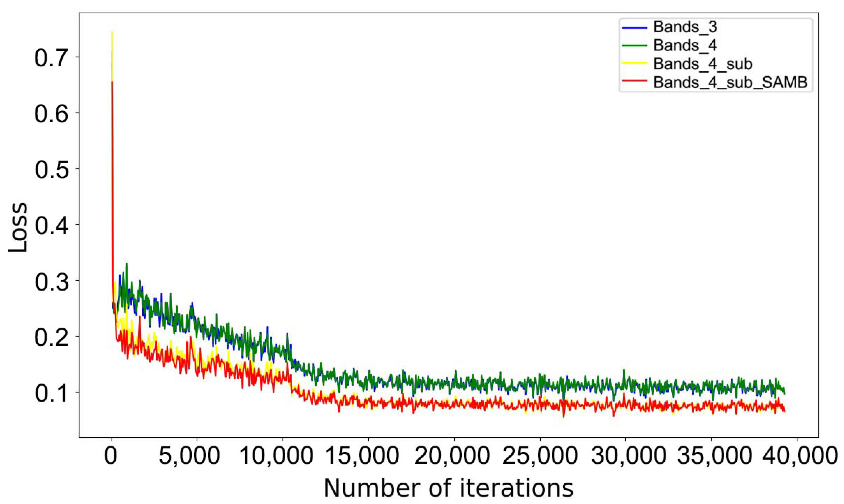
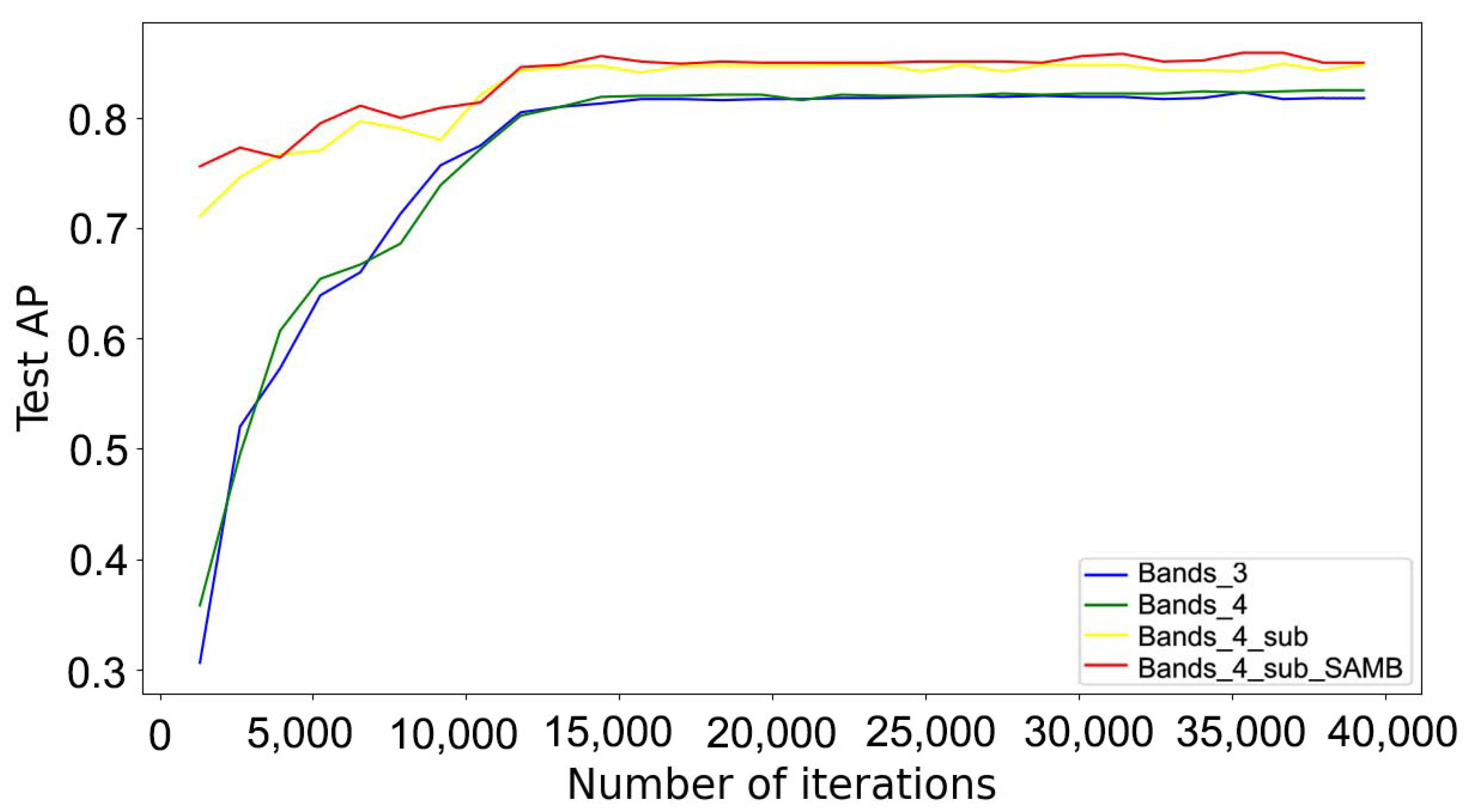
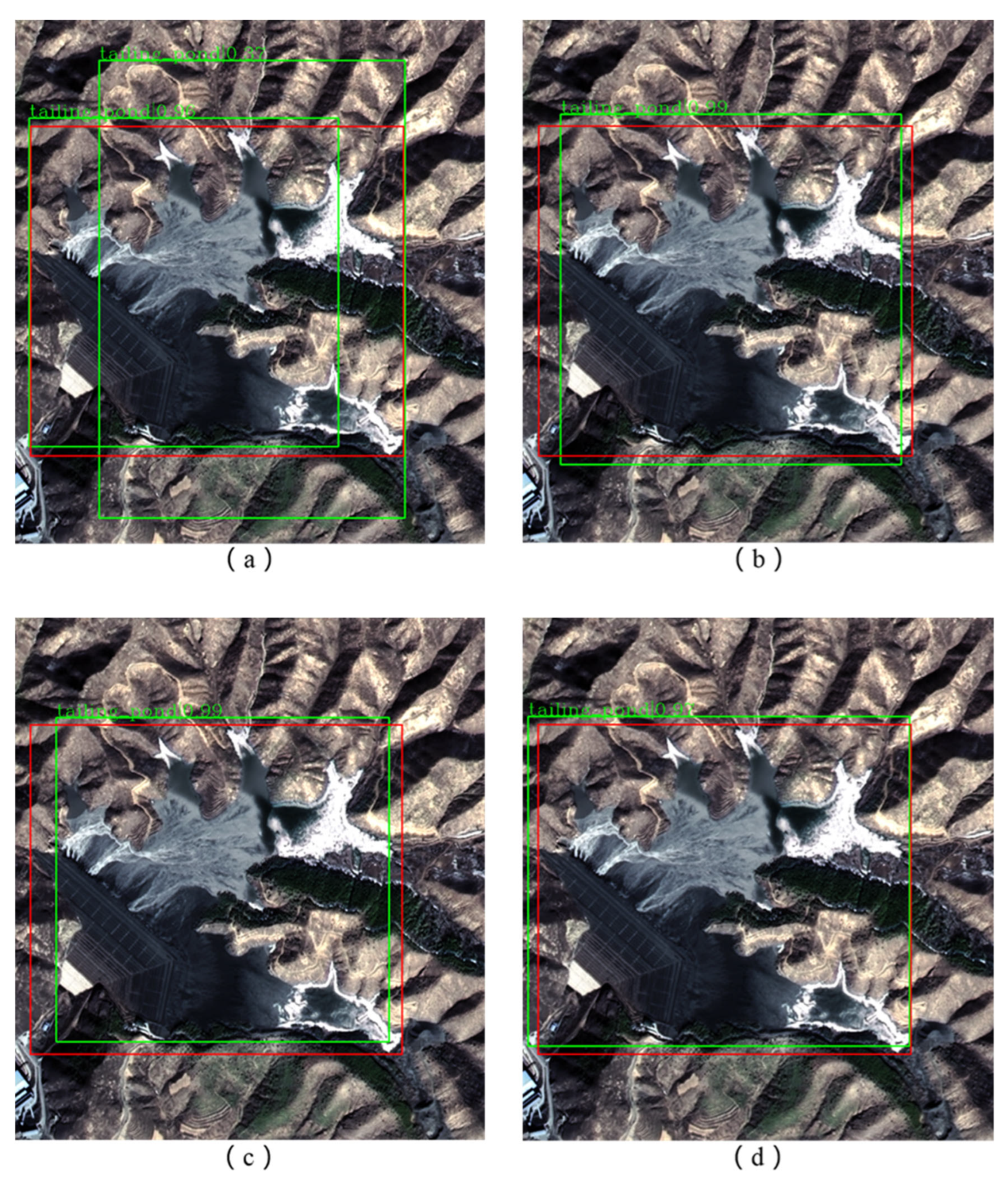
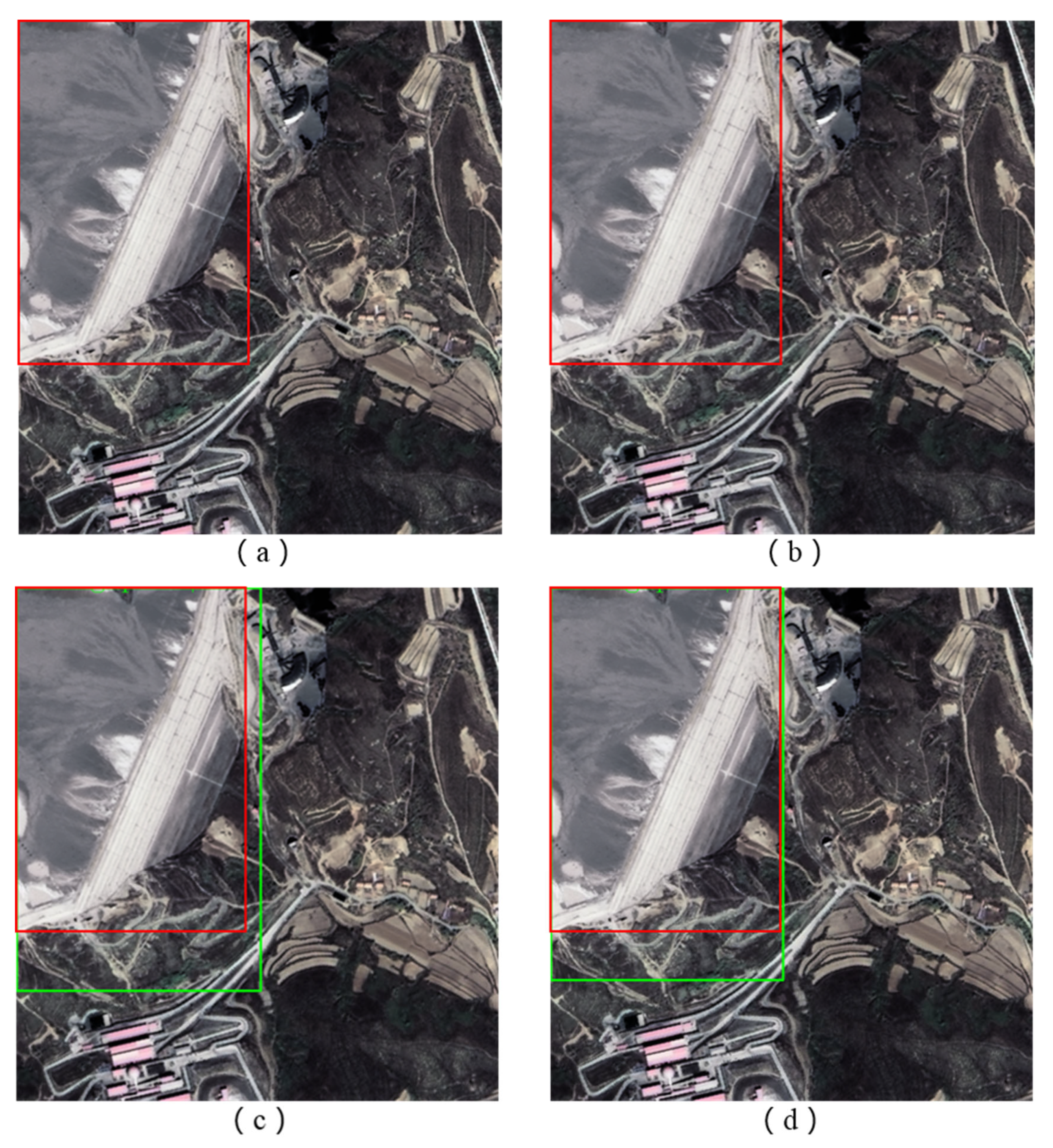
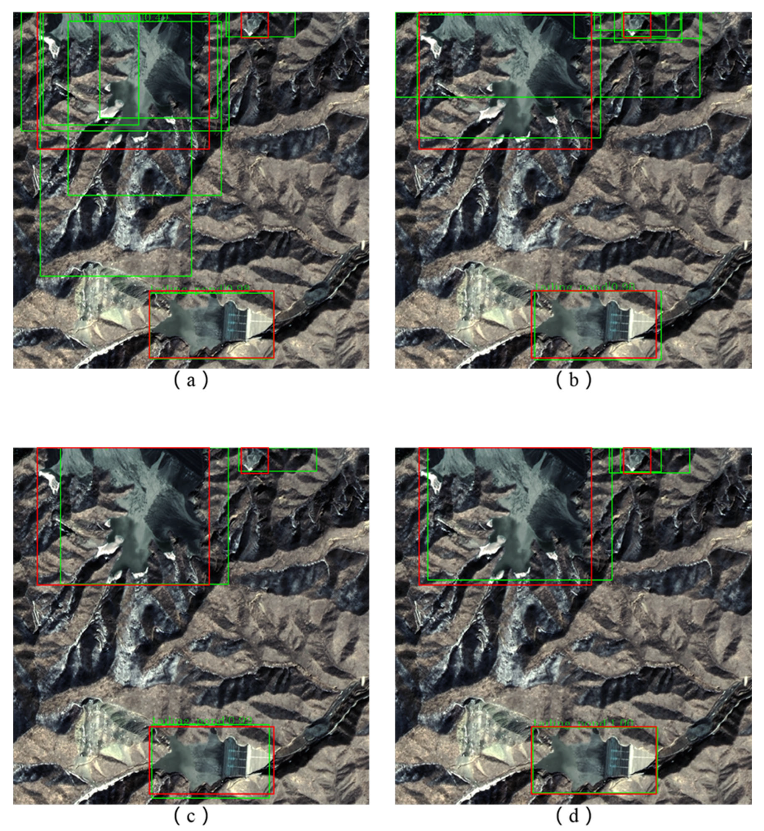
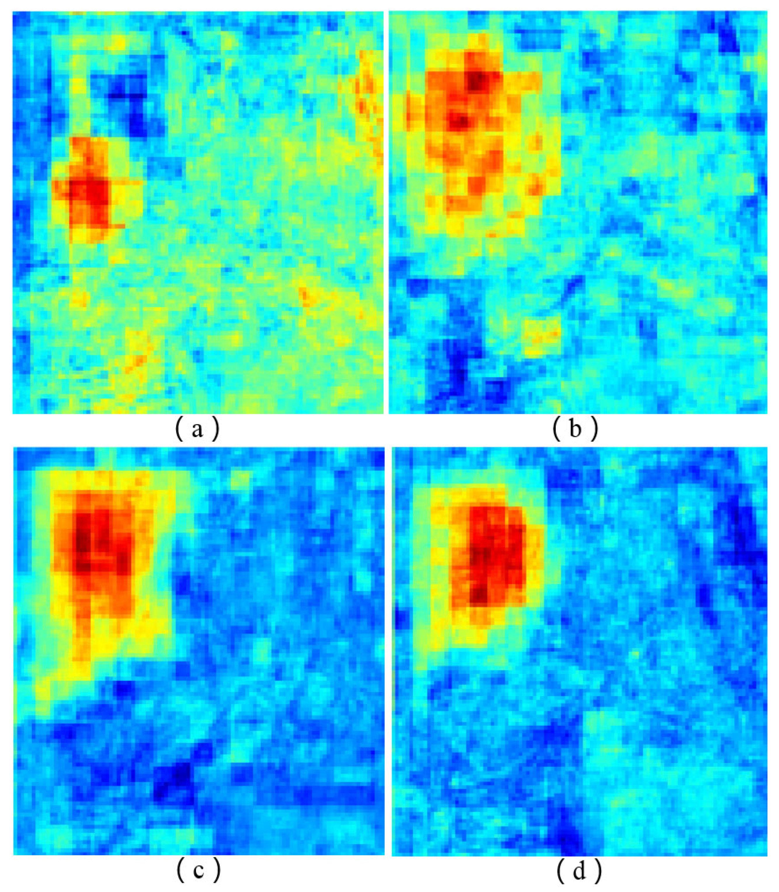
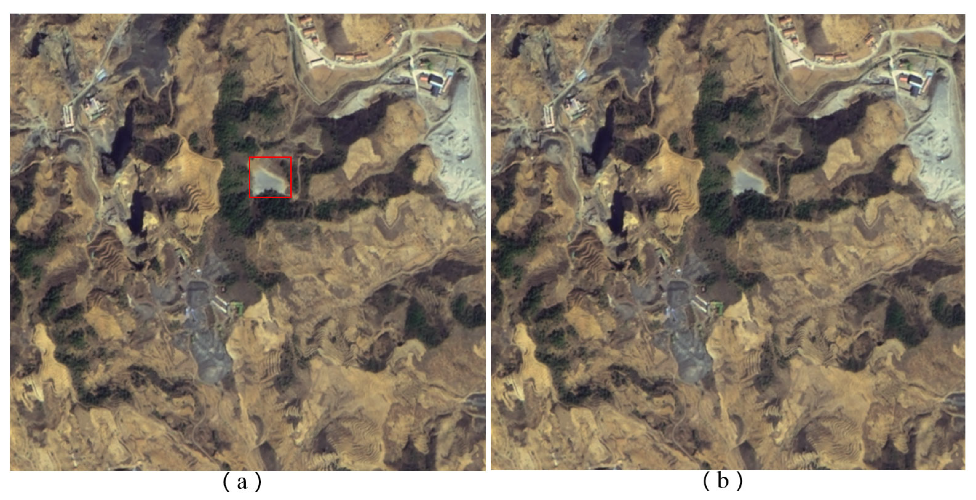
The network was trained using a 64-bit Ubuntu20.04LTs operating system and a NVIDIA GeForce GTX3080, using Xeon E5 CPU and CUDA version 11.1. The model trained 30 epochs of the training set. Stochastic gradient descent was used as the optimizer, the initial learning rate of the model was set to 0.02, momentum was set to 0.9, weight_decay was set to 0.0001, and the batch size was set to 2.

3. Results

Based on a sample dataset of tailings pond images from the GF-1 satellite, we improved the Faster R-CNN object detection model. We expanded the input from the three true-color bands to four multispectral bands and used the attention mechanism to recalibrate the contribution of the model input bands. Model improvement and training were gradually completed using a step-by-step transfer learning method.
The training loss curves for the different models shown in Figure 7 indicate that the curvilinear trends of Bands_3 and Bands_4 are remarkably similar, and the curvilinear trends of Bands4_sub and Bands4_sub_SAMB are quite similar, with excellent convergence in both cases. However, the loss values of the latter were significantly lower than those of the former.
The test precision curves for the various models shown in Figure 8 indicate that the curvilinear trends of Bands_3 and Bands_4 are quite similar, with gradually increasing and then stabilizing test precision. However, comparing Bands_3 and Bands_4 after NIR was added to the model indicated that the tailings pond detection precision did not significantly improve. It is evident from the Bands4_sub test precision curve that the initial test precision value was relatively high, and it rapidly increased further before stabilizing, reflecting the fact that the transfer learning method significantly improved the model training efficiency. Bands4_sub_SAMB used the attention mechanism to recalibrate the contribution of the original remote sensing image bands in the model. The initial test precision value was higher, and it quickly rose and reached a stable state. Compared with that of the Bands4_sub model, a more notable improvement was shown in the precision of tailings pond detection.
Table 3 shows specific model evaluation values. The Bands_3 model has an AP of 82.3%, and the Bands_4 model has a value of 82.5%, indicating that the latter did not effectively utilize the NIR band information to improve detection precision. After using the step-by-step transfer learning method, compared with that of the Bands_3 model, the AP and recall of the Bands_4_sub model greatly improved, increasing from 82.3% to 84.9% (up by 2.6%) and from 65.4% to 70.5% (up by 5.1%), respectively. The Bands_4_sub_SAMB model added the SAMB module to the feature extraction network of the Bands_4_sub model and recalibrated the contribution of the four bands in the image slices to further improve performance. The AP and recall increased by 1.0% and 1.4%, reaching 85.9% and 71.5%, respectively.
Looking at specific predicted tailings pond targets in Figure 9, (a) is the prediction result of the Bands_3 model, (b) is the prediction result of the Bands_4 model, (c) is the predictions result of the Bands_4_sub model, and (d) is the prediction result of the Bands_4_sub_SAMB model. In the images (as well as in Figure 10 and Figure 11), the red bounding box represents the GT of the tailings pond and the green bounding box represents the PT of the tailings ponds. In (a), the model predicted two different bounding boxes for one tailings pond, showing poor accuracy. In (b), (c), and (d), the models predicted one bounding box for the one tailings pond, and the accuracy of the PTs gradually improved.
Figure 10 shows that in (a) and (b), the tailings pond target was missed, but in (c) and (d), such missed detection was avoided. In addition, compared with the GT, the PT in (d) was significantly superior to that in (c). In Figure 12, (a)–(d) are feature heat maps of the corresponding images in Figure 10, with the improvement of the model, the characteristics of the tailings pond are gradually obvious and prominent, predictions are correspondingly better, which is consistent with the results in Figure 10.
Figure 11 shows that in (a), the tailings pond target in the top left of the image slice had multiple prediction results with poor accuracy, with some mistakenly detecting the shadow of the mountain and snow as part of the tailings pond. The smaller tailings pond target in the top right of the image slice had only one prediction result, but its accuracy was poor. In (b), the prediction result of the top-left tailings pond improved, but the prediction result of the smaller top-right tailings pond was worse than before, with multiple prediction bounding boxes appearing that showed poor accuracy. In (c) and (d), all the target prediction results significantly improved. In the comparison of (d) with (c), although the smaller top-right tailings pond had two prediction results in (d), one of the prediction results was more consistent with the GT; therefore, it showed greater accuracy.
Figure 13 shows that in (a), the red bounding box represents the GT of the small tailings pond, and (b) is the prediction result of all models. For some small tailings ponds, the improved method still cannot identify them. This may be because the tailings pond area is small, and the increase in NIR band information has a small contribution to the characteristic information. In view of this problem, we continued to improve it in the future study.

4. Discussion

Remote sensing image object detection, based on deep learning, primarily uses models from the field of computer vision. Transfer learning, hyperparameter adjustment, attention mechanisms, and other advanced deep learning techniques are used to improve models that adapt to the features of a target, enabling the highly precise and intelligent extraction of information. In the specific case of tailings ponds, most methods are based on improved deep learning object detection models and use information of the three true-color bands from high-resolution remote sensing imagery to intelligently extract tailings pond information. An advantage of remote sensing image data, however, is that it has more than three spectral bands, but few studies have considered how to utilize the rich information contained in the many spectral bands of remote sensing imagery to improve the precision of tailings ponds detection. To address this deficiency, using a sample dataset of tailings pond images from the Gaofen-1 satellite, our study has improved the deep learning object detection model known as Faster R-CNN by increasing its inputs from three true-color bands to four multispectral bands (adding the NIR band) as well as an attention mechanism to recalibrate the contributions of the four multispectral bands in the model. Subsequently, we used a step-by-step transfer learning method to gradually improve and train the model.
The training loss curves for the different models (Figure 7) show that Bands4_sub and Bands4_sub_SAMB have lower loss values than Bands_3 and Bands_4. The test precision curves for the various models (Figure 8) and the evaluation values of the various models (Table 3) show that the precisions of the Bands_3 and Bands_4 models are similar, indicating that Bands_4 model could not fully utilize the NIR band information, but the precision of the Bands_4_sub model significantly improved compared with that of Bands_3 and Bands_4, indicating that the step-by-step transfer learning method could effectively utilize NIR band information to significantly improve detection precision. The precision of the Bands_4_sub_SAMB model improved compared with that of Bands_4_sub, indicating that the recalibrated contribution of the input four bands further improved performance. The prediction results of different models also show that the proposed method can improve the accuracy of tailings pond detection and improve the mistaken detection and missed detection (Figure 9, Figure 10, Figure 11 and Figure 12).
Although the attention mechanism has been widely used in deep learning and remote sensing applications, it was used mostly to recalibrate extracted feature channels. There are few examples of using the attention mechanism on original remote sensing multi-band data. However, in this study, we adopted the method and improved detection precision with a relatively minor increase in parameters and calculations (e.g., single iteration time increased by only 0.095 s). Similarly, in contrast to the common transfer learning method, we adopted the step-by-step transfer learning method to fully utilize multispectral band information of remote sensing images to improve model performance.
The experimental results showed that the improved model could make full use of the NIR band information of GF-1 images to improve the precision of tailings pond detection. Compared with that of the triple-band input model, the AP and recall of tailings pond detection significantly improved in our model, with AP increasing from 82.3% to 85.9% and recall increasing from 65.4% to 71.9%. These results indicated that the model and method proposed in our study could utilize the multispectral band information of GF-1 images to improve the object detection precision for tailings ponds.

5. Conclusions

In this study, we used a sample dataset of tailings pond images from the GF-1 high-resolution Earth observation satellite. We improved the Faster R-CNN object detection model by increasing its inputs from the three true-color bands to four multispectral bands as well as using the attention mechanism to recalibrate their input contributions. A step-by-step transfer learning method was subsequently used to gradually improve and train the model. The experimental results showed that the improved model fully utilizes the NIR band information of the GF-1 images to improve tailings pond detection precision. Compared with that in the three true-color band input model, tailings pond detection AP and recall notably improved in our model, with the AP increasing from 82.3% to 85.9% (up by 3.6%) and recall increasing from 65.4% to 71.9% (up by 6.5%). The model and method proposed in this study made full use of the multispectral band information of GF-1 images to improve the accuracy of identifying tailings ponds. With the rapid development of remote sensing technology, more remote sensing image data are becoming increasingly available at higher spatial resolutions as well as with a greater number of spectral bands. Our research could serve as a reference for using multispectral band information from remote sensing images in the construction and application of a deep learning model. In the future, we will study the deep learning model based on multispectral remote sensing images to extract the boundary of tailings pond and determine the mineral types of tailings pond, and study the use of synthetic aperture radar data to monitor the tailings pond.

Author Contributions

Conceptualization, G.L. and D.Y.; methodology, D.Y. and H.Z.; software, D.Y. and K.L.; validation, D.Y., X.L. and H.Z.; formal analysis, L.Z.; investigation, H.L.; resources, F.Z.; data curation, X.L.; writing—original draft preparation, D.Y.; writing—review and editing, G.L. and D.Y.; visualization, D.Y.; supervision, G.L. and H.Z.; project administration, G.L.; funding acquisition, G.L. and H.Z. All authors have read and agreed to the published version of the manuscript.

Funding

This research was financially supported by Hainan Provincial Department of Science and Technology under Grant No. ZDKJ2019006; as well as the National Natural Science Foundation of China, grant number 41771397.

Acknowledgments

The authors would like to thank the editors and the anonymous reviewers for their helpful suggestions.

Conflicts of Interest

The authors declare no conflict of interest.

References

  1. Wang, T.; Hou, K.P.; Guo, Z.S.; Zhang, C.L. Application of analytic hierarchy process to tailings pond safety operation analysis. Rock Soil Mech. 2008, 29, 680–687. [Google Scholar]
  2. Yang, J.; Qin, X.; Zhang, Z.; Wang, X. Theory and Practice on Remote Sensing Monitoring of Mine; Surveying and Mapping Press: Beijing, China, 2011. [Google Scholar]
  3. Jie, L. Remote Sensing Research and Application of Tailings Pond–A Case Study on the Tailings Pond in Hebei Province; China University of Geosciences: Beijing, China, 2014. [Google Scholar]
  4. Zhou, Y.; Wang, X.; Yao, W.; Yang, J. Remote sensing investigation and environmental impact analysis of tailing ponds in Shandong Province. Geol. Surv. China 2017, 4, 88–92. [Google Scholar]
  5. Dai, Q.W.; Yang, Z.Z. Application of remote sensing technology to environment monitoring. West. Explor. Eng. 2007, 4, 209–210. [Google Scholar]
  6. Wang, Q. The progress and challenges of satellite remote sensing technology applications in the field of environmental protection. Environ. Monit. China 2009, 25, 53–56. [Google Scholar]
  7. Fu, Y.; Li, K.; Li, J. Environmental Monitoring and Analysis of Tailing Pond Based on Multi Temporal Domestic High Resolution Data. Geomat. Spat. Inf. Technol. 2018, 41, 102–104. [Google Scholar]
  8. Zhao, Y.M. Moniter Tailings Based on 3S Technology to Tower Mountain in Shanxi Province. Master’s Thesis, China University of Geoscience, Beijing, China, 2011; pp. 1–46. [Google Scholar]
  9. Wu, X.; Sahoo, D.; Hoi, S.C.H. Recent advances in deep learning for object detection. Neurocomputing 2020, 396, 39–64. [Google Scholar] [CrossRef] [Green Version]
  10. Bai, T.; Pang, Y.; Wang, J.; Han, K.; Luo, J.; Wang, H.; Lin, J.; Wu, J.; Zhang, H. An Optimized Faster R-CNN Method Based on DRNet and RoI Align for Building Detection in Remote Sensing Images. Remote Sens. 2020, 12, 762. [Google Scholar] [CrossRef] [Green Version]
  11. Ren, S.; He, K.; Girshick, R.; Sun, J. Faster R-CNN: Towards real-time object detection with region proposal networks. Adv. Neural Inf. Process. Syst. 2015, 28, 91–99. [Google Scholar] [CrossRef] [Green Version]
  12. Zambanini, S.; Loghin, A.-M.; Pfeifer, N.; Soley, E.M.; Sablatnig, R. Detection of Parking Cars in Stereo Satellite Images. Remote Sens. 2020, 12, 2170. [Google Scholar] [CrossRef]
  13. Wang, C.; Chang, L.; Zhao, L.; Niu, R. Automatic Identification and Dynamic Monitoring of Open-Pit Mines Based on Improved Mask R-CNN and Transfer Learning. Remote Sens. 2020, 12, 3474. [Google Scholar] [CrossRef]
  14. He, K.; Gkioxari, G.; Dollár, P.; Girshick, R. Mask R-CNN. In Proceedings of theIEEE International Conference on Computer Vision (ICCV), Venice, Italy, 22–29 October 2017; pp. 386–397. [Google Scholar]
  15. Machefer, M.; Lemarchand, F.; Bonnefond, V.; Hitchins, A.; Sidiropoulos, P. Mask R-CNN Refitting Strategy for Plant Counting and Sizing in UAV Imagery. Remote Sens. 2020, 12, 3015. [Google Scholar] [CrossRef]
  16. Zhao, K.; Kang, J.; Jung, J.; Sohn, G. Building extraction from satellite images using mask R-CNN with building boundary regularization. In Proceedings of the IEEE Conference on Computer Vision and Pattern Recognition Workshops, Salt Lake City, UT, USA, 18–22 June 2018. [Google Scholar]
  17. Li, Q.; Chen, Z.; Zhang, B.; Li, B.; Lu, K.; Lu, L.; Guo, H. Detection of tailings dams using high-resolution satellite imagery and a single shot multibox detector in the Jing–Jin–Ji Region, China. Remote Sens. 2020, 12, 2626. [Google Scholar] [CrossRef]
  18. Liu, W.; Anguelov, D.; Erhan, D.; Szegedy, C.; Reed, S.; Fu, C.Y.; Berg, A.C. Ssd: Single shot multibox detector. In Proceedings of the European Conference on Computer Vision, Amsterdam, The Netherlands, 8–16 October 2016; pp. 21–37. [Google Scholar]
  19. Lyu, J.; Hu, Y.; Ren, S.; Yao, Y.; Ding, D.; Guan, Q.; Tao, L. Extracting the Tailings Ponds from High Spatial Resolution Remote Sensing Images by Integrating a Deep Learning-Based Model. Remote Sens. 2021, 13, 743. [Google Scholar] [CrossRef]
  20. Bochkovskiy, A.; Wang, C.; Liao, H. YOLOv4: Optimal Speed and Accuracy of Object Detection. arXiv 2020, arXiv:2004.10934v1. [Google Scholar]
  21. Yan, K.; Sheng, T.; Chen, Z.; Yan, H. Automatic extraction of tailing pond based on SSD of deep learning. J. Univ. Chin. Acad. Sci. 2020, 37, 360–367. [Google Scholar]
  22. Zhang, K.; Chang, Y.; Pan, J.; Lu, K.; Zan, L.; Chen, Z. Multi-Task-Branch Framework for Tailing Pond of Tangshan City. J. Henan Polytech. Univ. (Nat. Sci.). 2020, 10, 1–11. [Google Scholar]
  23. Yan, D.; Li, G.; Li, X.; Zhang, H.; Lei, H.; Lu, K.; Cheng, M.; Zhu, F. An Improved Faster R-CNN Method to Detect Tailings Ponds from High-Resolution Remote Sensing Images. Remote Sens. 2021, 13, 2052. [Google Scholar] [CrossRef]
  24. Yu, G.; Song, C.; Pan, Y.; Li, L.; Li, R.; Lu, S. Review of new progress in tailing dam safety in foreign research and current state with development trend in China. Chin. J. Rock Mech. Eng. 2014, 33, 3238–3248. [Google Scholar]
  25. Lin, T.Y.; Dollar, P.; Girshick, R.; He, H.; Hariharan, B.; Belongie, S. Feature pyramid networks for object detection. arXiv 2017, arXiv:1612.03144. [Google Scholar]
  26. Chaudhari, S.; Mithal, V.; Polatkan, G.; Ramanath, R. An attentive survey of attention models. arXiv 2020, arXiv:1904.02874. [Google Scholar] [CrossRef]
  27. Mnih, V.; Heess, N.; Graves, A.; Kavukcuoglu, K. Recurrent models of visual attention. In Proceedings of the Advances in Neural Information Processing Systems (NIPS), Montréal, QC, Canada, 8–13 December 2014; pp. 2204–2212. [Google Scholar]
  28. Bahdanau, D.; Cho, K.; Bengio, Y. Neural machine translation by jointly learning to align and translate. arXiv Prepr. 2014, arXiv:1409.0473. [Google Scholar]
  29. Li, Y.; Huang, Q.; Pei, X.; Jiao, L.; Ronghua, S. RADet: Refine feature pyramid network and multi-layer attention network for arbitrary-oriented object detection of remote sensing images. Remote Sens. 2020, 12, 389. [Google Scholar] [CrossRef] [Green Version]
  30. Redmon, J.; Divvala, S.; Girshick, R.; Farhadi, A. You Only Look Once: Unified, Real-Time Object Detection. In Proceedings of the 2016 IEEE Conference on Computer Vision and Pattern Recognition, Las Vegas, NV, USA, 27–30 June 2016; pp. 779–788. [Google Scholar]
  31. Hu, J.; Zhi, X.; Shi, T.; Zhang, W.; Cui, Y.; Zhao, S. PAG-YOLO: A Portable Attention-Guided YOLO Network for Small Ship Detection. Remote Sens. 2021, 13, 3059. [Google Scholar] [CrossRef]
  32. Hu, J.; Shen, L.; Sun, G. Squeeze-and-excitation Networks. In Proceedings of the 2018 IEEE Conference on Computer Vision and Pattern Recognition, Salt Lake City, UT, USA, 18–23 June 2018; pp. 7132–7141. [Google Scholar]
  33. He, K.; Zhang, X.; Ren, S.; Sun, J. Deep Residual Learning for Image Recognition. In Proceedings of the IEEE Conference on Computer Vision and Pattern Recognition, Las Vegas, NV, USA, 27–30 June 2016. [Google Scholar]
  34. Zhang, B.; Shi, Z.; Zhao, X.; Zhang, J. A Transfer Learning Based on Canonical Correlation Analysis Across Different Domains. Chin. J. Comput. 2015, 38, 1326–1336. [Google Scholar]
  35. Pan, S.J.; Yang, Q. A survey on transfer learning. IEEE TKDE 2010, 22, 1345–1359. [Google Scholar] [CrossRef]
  36. Yosinski, J.; Clune, J.; Bengio, Y.; Lipson, H. How transferable are features in deep neural networks? Adv. Neural Inf. Processing Syst. 2014, 27, 3320–3328. [Google Scholar]
Figure 1. Locations of tailings pond samples.
Remotesensing 14 00103 g001
Figure 2. GF-1 image of sample tailings pond features, with the ground truth bounding boxes shown in red: (a) stockpile type; (b) hillside type; and (c) cross-valley type.
Remotesensing 14 00103 g002
Figure 3. Proposed optimized network structure.
Remotesensing 14 00103 g003
Figure 4. Slice attention mechanism block.
Remotesensing 14 00103 g004
Figure 5. Proposed feature extraction network.
Remotesensing 14 00103 g005
Figure 6. Step-by-step transfer learning.
Remotesensing 14 00103 g006
Figure 7. Training loss curves for different models.
Remotesensing 14 00103 g007
Figure 8. Test precision curves for different models.
Remotesensing 14 00103 g008
Figure 9. Improved accuracy of tailings pond detection. (a) prediction result of the Bands_3 model, (b) prediction result of the Bands_4 model, (c) prediction result of the Bands_4_sub model, (d) prediction result of the Bands_4_sub_SAMB model, the red bounding box represents the GT of the tailings pond and the green bounding box represents the PT of the tailings pond.
Remotesensing 14 00103 g009
Figure 10. Improvement in missed detection and detection accuracy. (a) prediction result of the Bands_3 model, (b) prediction result of the Bands_4 model, (c) prediction result of the Bands_4_sub model, (d) prediction result of the Bands_4_sub_SAMB model, the red bounding box represents the GT of the tailings pond and the green bounding box represents the PT of the tailings pond.
Remotesensing 14 00103 g010
Figure 11. Improvement in mistaken detections and detection accuracy. (a) prediction result of the Bands_3 model, (b) prediction result of the Bands_4 model, (c) prediction result of the Bands_4_sub model, (d) prediction result of the Bands_4_sub_SAMB model, the red bounding box represents the GT of the tailings pond and the green bounding box represents the PT of the tailings pond.
Remotesensing 14 00103 g011
Figure 12. Feature heat maps of different models. (a) feature heat map of the Bands_3 model, (b) feature heat map of the Bands_4 model, (c) feature heat map of the Bands_4_sub model and (d) feature heat map of the Bands_4_sub_SAMB model.
Remotesensing 14 00103 g012
Figure 13. Small tailings pond target missed detection. (a) the red bounding box represents the GT of the small tailings pond and (b) the prediction results of all models.
Remotesensing 14 00103 g013
Table 1. Parameters of the 2 m panchromatic/8 m multispectral cameras.
Spectral BandWavelength (um)Spatial Resolution
(m)
Swath Width at Nadir
(km)
Revisit Time
(d)
Pan0.45–0.9026941
Blue0.45–0.5286941
Green0.52–0.59
Red0.63–0.69
NIR0.77–0.89
Table 2. Sample set information.
Sample SetSpatial
Resolution (m)
Bands
Number
Size
(Pixels)
Data Type
(bit)
Slices Number
Train set2.041024 × 102481509
Test set2.041024 × 10248369
Table 3. Test results for different models.
TypeAP (%)Recall (%)Iteration Time (s)
Bands_382.365.40.387
Bands_482.564.60.390
Bands_4_sub84.970.50.392
Bands_4_sub_SAMB85.971.90.487
Publisher’s Note: MDPI stays neutral with regard to jurisdictional claims in published maps and institutional affiliations.

