Abstract
Semantic segmentation has been a fundamental task in interpreting remote sensing imagery (RSI) for various downstream applications. Due to the high intra-class variants and inter-class similarities, inflexibly transferring natural image-specific networks to RSI is inadvisable. To enhance the distinguishability of learnt representations, attention modules were developed and applied to RSI, resulting in satisfactory improvements. However, these designs capture contextual information by equally handling all the pixels regardless of whether they around edges. Therefore, blurry boundaries are generated, rising high uncertainties in classifying vast adjacent pixels. Hereby, we propose an edge distribution attention module (EDA) to highlight the edge distributions of leant feature maps in a self-attentive fashion. In this module, we first formulate and model column-wise and row-wise edge attention maps based on covariance matrix analysis. Furthermore, a hybrid attention module (HAM) that emphasizes the edge distributions and position-wise dependencies is devised combing with non-local block. Consequently, a conceptually end-to-end neural network, termed as EDENet, is proposed to integrate HAM hierarchically for the detailed strengthening of multi-level representations. EDENet implicitly learns representative and discriminative features, providing available and reasonable cues for dense prediction. The experimental results evaluated on ISPRS Vaihingen, Potsdam and DeepGlobe datasets show the efficacy and superiority to the state-of-the-art methods on overall accuracy (OA) and mean intersection over union (mIoU). In addition, the ablation study further validates the effects of EDA.
1. Introduction
Semantic segmentation, a fundamental task for interpreting remote sensing imagery (RSI), is currently essential in various fields, such as water resource management [1,2], land cover classification [3,4,5], urban planning [6,7] and precision agriculture [8,9] and so forth. This task strives to produce a raster map that refers to an input image by assigning a categorical label to every pixel [10]. The observed objects and terrain information are easily recognized and analyzed with the labeled raster map, contributing to structuralized and readable knowledge. However, the reliability and availability of the transformed knowledge are tremendously conditioned on the accuracy of semantic segmentation.
Conventional segmentation methods of remote sensing imagery are essentially implemented by statistically analyzing the prior distributions. For example, Arivazhagan et al. [11] extracted and combined wavelet statistical features and co-occurrence features, characterizing the textures at different scales. As a result, the experiments on monochrome images achieved comparable performance. For segmenting plant leaves, Gitelson A. and Merzlyak M. [12] developed a new spectral index, green normalized difference vegetation index (GNDVI), based on the spectral properties. Although it works well, the specifying spectral range occupation leads to finite application. Likewise, the normalized difference index for ASTER 5–6 was devised incorporating several vegetation indices [13]. This index helps the model segment the major crops by grouping crop fields with similar values. Subsequently, Blaschke T. summarized these methods as object-based image analysis for remote sensing (OBIA), utilizing spectral and spatial information in an integrative fashion [14]. To sum up, the traditional methods are target-specific and spectra-fixed, making the segmentation model not robust. Moreover, concerning the arrival of the big data era, this kind of approach is far from usable when individually working on the task.
More recently, machine learning models were extensively applied to classify pixels following handcrafted features. For example, Yang et al. [15] captured texture and context by fusing Texton descriptor and the association potential in the conditional random field (CRF) framework. Mountrakis et al. [16] reviewed the support vector machine (SVM) classifiers in remote sensing. SVM resorts to a small number of training samples while reaching comparable accuracy. Random forest (RF) also exhibits its strong ability to classify remote sensing data with high dimensionality and multicollinearity [17]. Nevertheless, conventional machine learning methods are not automative and intelligent. Although the efficiency is acceptable, the accuracy is criticized, especially for multi-sensor and multi-platform data.
Since the successful development of convolutional neural networks (CNNs), numerous studies have examined the application of CNNs. CNNs have demonstrated the powerful capacity of feature extraction and object representations compared with traditional methods in machine learning. One of the most significant breakthroughs was the fully convolutional neural network (FCN) [18]. FCN is the first end-to-end framework, allowing the deconvolution layer to recover feature maps. However, the major drawback is the accompanying information loss in shrinking and dilating features’ spatial size. To alleviate the transformation loss, an encoder-decoder segmentation network (a.k.a. SegNet) [19] was designed with a symmetrical architecture. In the encoder, the indexes of the largest pixels are recorded. As to the corresponding decoder stage, the recorded pixels are re-assigned to the same position. Similarly, U-Net [20] retains the detailed information better with the skip connections between encoder and decoder. The initial implementation of medical images verifies the remarkable progress compared to FCN and SegNet. In addition, these works revealed that comprehensively capturing contextual information enables accurate segmentation results.
Endeavoring to enrich the learnt representations with contextual information, the atrous convolution was proposed [21]. This unit adjusts a rate to convolve the adjacent pixels for generating the central position’s representations. DeepLab V2 [22] built a novel atrous spatial pyramid pooling (ASPP) module to sample features at different scales. Furthermore, DeepLab V3 [23] integrated global average pooling to embed more helpful information. Considering the execution efficiency, DeepLab V3+ [24] opted for Xception as the backbone and depth-wise convolution. Unfortunately, enlarging the receptive field will cause edge distortions, where the surrounding pixels are error-prone.
Regarding the geographic objects’ properties of RSI, context aggregation is advocated. Even for the same class, the scale of the optimal segments is different. Therefore, the context aggregation methods are devoted to minimizing the heterogeneity of intra-class objects and maximize the heterogeneity of inter-class objects by fusing the multi-level feature maps at various scales. For example, Zhang et al. [25] designed a multi-scale context aggregation network. This network encodes the raw image by the high-resolution network (HRNet) [26], in which four parallel branches are presented to generate four sizes of feature maps. Then, these are enhanced with corresponding tricks before concatenation. Results on the ISPRS Vaihingen and Potsdam datasets are competitive. Coincidentally, a multi-level feature aggregation network (MFANet) [27] was proposed with the same motivation. Two modules, channel feature compression (CFC) and multi-level feature aggregation upsample (MFAU), were designed to reduce the loss of details and make the edge clear. Moreover, Wang et al. [28] defined a cost-sensitive loss function in addition to fuse multi-scale deep features.
Alternatively, the attention mechanism was initially applied to boost the performance for labeling natural images. SENet [29] built a channel-wise attention module that recalibrates the channel weights with learnt relationships between arbitrary channels. In this way, SENet could help the network pay more attention to the channels with complementary information. Concerning spatial and channel correlations simultaneously, CBAM [30] and DANet [31] were implemented and achieved perceptible improvements results on natural image data. The following proposed self-attention fashion further optimizes the representations. The non-local neural network [32] was proposed to learn the position-wise attention maps both in spatial and channel domains. Regarding the capability of self-attentively modeling the long-range dependencies, ACFNet [33] offered a coarse-to-fine segmentation pipeline. The self-attention module also inspired the proposal of OCRNet [34], in which relational context is extracted and fed for prediction, sharping object’s boundaries.
While the attention modules are transplanted to RS, the diversity and easily-confused geo-objects are well-distinguished than before [35]. To this end, many variant networks that introduce attention rationale were investigated. CAM-DFCN [36] incorporates channel attention to FCN architecture for using multi-modal auxiliary data to enhance the distinguishability of features. HMANet [37] adaptively captures the correlations that lie in space, channel and category domains effectively. This model benefits from the extensible self-attention mechanism. Li et al. [38] disclosed that the most challenging task is recognizing and accepting the diverse intra-class variance and inconspicuous inter-class variance. Thereby, the SCAttNet integrates the spatial and channel attention to form a lightweight yet efficient network. More recently, Lei et al. [39] proposed LANet, which bridges the gap between high- and low-level features by embedding the local focus from high-level features with the designed patch attention module. In terms of the successful cases of attention-based methods, it is concluded that the attention modules can strengthen the separability of learned representations, making the error-prone objects more distinguishable. Marmanis et al. [40] pointed out that edge regions contain implicated semantically meaningful boundaries. However, the existing attentive techniques equally learn the representation for every pixel. As a result, the surrounding pixels of edges are easily misjudged, tending to the blurry edge region even rising high uncertainties of long-distance pixels.
To perceive and transmit edge knowledge, Marmanis et al. combined semantically informed edge detection with encoder-decoder architecture. Then, the class boundaries are explicitly modeled, adjusting the training phase. This memory-efficient method yields more than 90% accuracy on the ISPRS Vaihingen benchmark. Afterward, PEGNet [41] presented a multipath atrous convolution module to generate dilated edge information across canny and morphological operations. Thus, the edge-region maps help the network identify the pixels around edges with high consistency. In addition, a recalibrate module is regulated by training loss to guide the misclassified pixels, reporting an overall accuracy of more than 91% of the Vaihingen dataset.
To sum up, the commonly used combination of boundary detector and segmentation network is complex with much more time-costs. The independent boundary detector requires corresponding loss computation and an embedded interface of the trunk network. In addition, the existing methods are far from adaptively extracting and injecting edge distributions. Hence, the purpose of this study includes two aspects: (1) the edge knowledge is urgent to be explicitly modeled and incorporated into learnt representations, facilitating the network’s discriminative capability in labeling pixels that position at marginal areas; (2) the extraction and incorporation of edge distributions should be learnable and end-to-end trainable without breaking the inherent spatial structure.
Generally, CNNs have demonstrated superiority in segmenting remote sensing imagery by learning local patterns. Nevertheless, the remote sensing imagery always covers wide-range areas and observes various ground objects. This property makes the networks insufficient and leads to the degradation of accuracy. Furthermore, although the attention modules brought astounding improvements by learning contextual information, equally processing edges induce blur around boundaries, which indirectly causes massive misclassified pixels. Hence, it is necessary to incorporate the edge distributions to assist the network in enhancing edge delineation and recognizing various objects. Motivated by the attention mechanism and two-dimensional principal component analysis (2DPCA) diagram [42], we found that injecting edge distributions with a learnable way is available. Therefore, in this study, we firstly formulate and re-define the covariance matrix inspired by 2DPCA. To refine the representations, two perspectives of efforts are devoted. One is learning edge distributions modelled by the re-defined covariance matrix following the inherently spatial structure of encoded feature maps. The other is the employment of the non-local block, a typical self-attention module with high efficiency, to enhance the representations with local and global contextual information. Therefore, the hybrid strategy makes the segmentation network determine the dominating features and filter irrelevant noise. In summary, the contributions are as follows,
- (1)
- Inspired by the image covariance analysis of 2DPCA, the covariance matrix (CM) is re-defined with learnt feature maps in the network. Then, the edge distribution attention module (EDA) is devised based on the covariance matrix analysis, modeling the dependencies of edge distributions in a self-attentive way explicitly. Through the column-wise and row-wise edge attention maps, the vertical and horizontal relationships are both quantified and leveraged. Specifically, in EDA, the handcrafted feature is successfully combined with learnt ones.
- (2)
- A hybrid attention module (HAM) that emphasizes the edge distributions and position-wise dependencies is devised. Thereby, more complementary edge and contextual information are collected and injected. This module supports independent and flexible embedding by a parallel architecture.
- (3)
- A conceptually end-to-end neural network, named edge distribution-enhanced semantic segmentation neural network (EDENet), is proposed. EDENet hierarchically integrates HAM to generate representative and discriminative encoded features, providing available and reasonable cues for dense prediction.
- (4)
- Extensive experiments are conducted on three datasets, ISPRS Vaihingen [43] and Potsdam [44] and DeepGlobe [45] benchmarks. In addition, the results indicate that EDENet is superior to other state-of-the-art methods. In addition, the ablation study further tests the efficacy of EDA.
The remainders of this paper are organized as follows: Section 2 introduces the related works, including attention mechanism, 2DPCA and non-local block. Section 3 concretely presents the devised framework and pipeline of sub-modules. Section 4 quantitatively and qualitatively evaluates the proposed method on both aerial and satellite images. Finally, the conclusions are drawn in Section 5.
2. Preliminaries
2.1. Attention Mechanism
Attention mechanism (AM) derives from human cognition process, selectively focusing on two main targets: (1) deciding whether the interdependence between the input elements should be considered; (2) quantifying how much attention/weight should be put to these elements. Since being successfully applyied to natural language processing (NLP) [46], sundry visual tasks have reaped many benefits, such as image classification, object detection, scene parsing and semantic segmentation. [47,48,49,50]. The foremost advantage is that AM can be adaptively generalized to all visual tasks by easily embedding to backbones.
Correspondingly, two tactics are adopted to build the attention modules in vision tasks: (1) devising an independent branch in a neural network to highlight the strong-correlated local regions or specific channels’ feature maps, filtering the irrelevant information, such as [51,52]; (2) completely modeling the dependencies both in spatial and channel domains, in which the attention matrix that explicitly quantifies the correlations is formed to reinforce the semantic knowledge, such as [31,32,53].
In addition, Yang et al. [54] presented a significant analysis and discussion on the one-step attention modules. They revealed that the suboptimal performance is obtained accompanying by incorporated noise in the irrelevant regions or pixels. In an attempt to eliminate the interferences, CCNet [53] repeatedly used attention modules that designed by Yang et al. to promote the feature maps.
Instead of stacking or listing attention modules, the correlation-based self-attention mechanism was proposed, which expresses the powerful capability to capture spatial and channel-wise dependencies simultaneously [31]. In addition, a medical image semantic segmentation network was deeply inspired by this idea [49]. Similarly, non-local neural networks [32], ACFNet [33] and OCRNet [34] were devised with desired improvements on many datasets. For capturing hierarchical features, Li et al. [55] proposed a pyramid attention network (PAN), combining attention module and spatial pyramid to extract precisely dense features. Meanwhile, Zhu et al. [56] have proved that the attention mechanism has great potential in promoting boundary awareness.
To determine the effects of edge information in a learnable style, self-attention heaves into sight. Provided that the feature maps’ edge distributions are substantially available and undistorted, we can use covariance matrix analysis to quantify the prior edges in feature maps followed by learning attentive correlations, generating edge distribution attentive maps.
2.2. Revisiting 2DPCA
To unravel and learn the edge distribution, it is essential to explain how to represent the edge information in the learnt feature maps. As discussed above, our idea of building edge distribution attention module is inspired by the 2DPCA [42], which provides a simple yet efficient way to describe the prior distributions by covariance matrix analysis [57]. This part is presented to revisit the principal theory of 2DPCA for understanding how covariance matrix analysis regulates the images.
An arbitrary image can be characterized as a high-dimensional matrix, such as a natural RGB image is numerically a three-dimensional matrix. Practically, for the sake of understanding, the explanation starts with a single channel image. Let A denote an input image with single dimension and , where and represent row and column respectively. Initially, the vector is designed to project following the linear transformation,
where is an -dimensional unitary column vector, is projected vector with dimensions. As can be seen, is defined as the projected feature vector of image . Then, to measure the discriminatory power of , the total scatter of projected samples are used and characterized by the trace of covariance matrix. Therefore,
where represents the covariance matrix of projected feature vectors, is a function to calculate the trace of matrix and denotes the total scatter. Regarding the physical significance, the purpose is to project all the samples by a particular projection direction. If all the pixels are projected, the total scatter goes maximized. Furthermore, is ascertained as follows,
where denotes the unitary matrix and means the transpose of . Consequently, the image covariance matrix is formed as
where represents the image covariance matrix and is unequivocally nonnegative definite matrix. When extending to more images with the same spatial size, the average of all the training samples can be obtained. Here, the is re-inferred as
where is the average of all the training samples and is the number of samples. Alternatively, Equation (2) is transformed to
where is an -dimensional unitary column vector. The optimal leads to maximized . In other words, the eigenvector of conforms to the largest eigenvalue [53]. A single optimal projection axis is impossible. So, a set of that subject to the orthonormal constraints and maximizing the criterion is presented:
After finding the optimal projection vectors, these vectors are then delivered to extract the features. Given the image sample ,
Thus, the feature matrix is produced with , where denotes the principal component vectors.
In general, 2DPCA creates a projection process to extract the feature matrix in virtue of covariance matrix analysis. This finding makes all the samples enlarged along with the principal directions and shrank along with the non-principal ones.
2.3. Non-Local Block
As a typical self-attention block, non-local block (NLB) captures position-wise correlations with comparative lower time and space occupation. Originally, non-local—a classical filtering algorithm—computes a weighted mean of all pixels, allowing distant pixels to contribute to the specific pixel along with patch appearance similarity. Following the idea of non-local means, the non-local block in neural networks is invented.
As detailed in Figure 1, the pipeline of the non-local block is presented. In the beginning, three convolutions are implemented to produce three multifarious feature maps. Then, they are reshaped to the given dimensionality. Next, the flattened features of the first and second branches are used to calculate similarity, generating positional self-attentive maps via matrix multiplication. At last, one more matrix multiplication is applied to the flattened features of the third branch and the self-attentive map to inject the position-wise dependencies to the raw features. Towards the end, a reshape operation followed by 1 × 1 convolutions is experienced to recover the learnt representations. Therefore, the out sophisticated features retain the same dimensionality as the input.
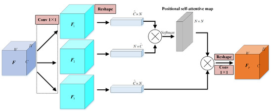
Figure 1.
Illustration of non-local block.
Formally, the NLB is described as
where denotes the position-wise attention enhanced feature maps and is the attention maps that built upon the first two branches’ feature maps.
Intuitively, the flow path of NLB is clear and concise. On the one hand, the position-wise dependencies are modeled and injected by matrix multiplications. On the other hand, the pipeline shows that NLB is flexible. Because NLB only relies on the input feature maps. As a result, NLB presents its significance in embedding to various networks for different visual tasks. In the rest of this paper, NLB is termed as SAM in the proposed framework.
3. The Proposed Method
3.1. Overview
In contrast to ResUNet-a [58], SCAttNet [38] is inexpensive in time and space costs. Nonetheless, the results raise slightly. The finding indicates that the attention-based models are available for improving learnt representations of RSI. We conclude that these two studies ignore the prior distribution information of edge/contour, delineating object entities with blurs.
This part below illustrates and explains the overall framework of EDENet. Essentially, as presented in Figure 2, its shape looks like a variant of U-Net, based on encoder-decoder architecture. As for the encoder stage, in this study, many standard backbones are allowable, such as ResNet, MobileNet and DenseNet. In addition, the implementation details will be further discussed in the next section. Correspondingly, the decoder symmetrically recovers the feature maps for dense prediction. Instead of using unitary feature maps that output from the encoder, feature maps with multi-spatial size are concatenated for providing important contextual cues, including semantic, spatial and edge clues. To alleviate the structural loss, the HAMs are hierarchically embedded to boost the relevant feature maps. Noticeably, HAM hybridizes SAM and EDA parallelly, enriching the contextual dependencies and edge information simultaneously. The following is a brief description of HAM and EDA, including topological architecture and formalization.
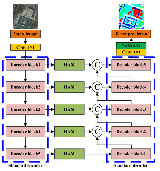
Figure 2.
Overall framework of EDENet.
3.2. Edge Distribution Attention Module
As previously stated, edges are of great importance for segmentation. Suppose that the more accurate boundary is delineated. Naturally, the localization of segments/objects is given. Existing networks, such as SegNet, U-Net and DeepLab V3+, have pointed out that both the accuracy of localization and recognition are equally helpful to the performance. However, these approaches rest on the convolutions’ self-regulating ability, which is uncontrollable and variable. Especially for RSI, understanding and modeling the edge distributions impacts more on segmentation. As we all know, the objects of RSI are various, diverse and complex. The pixels lie in the central parts of objects always correctly labeled, while the pixels around edges are easily misclassified. The inconsistent, mixing and heterogeneous edge regions cause this, presenting massive error-prone pixels. Although the recently proposed ResUNet-a and SCAttNet are implemented to produce more consistent and smooth boundaries from enlarging the receptive field and paying attention to dependencies, the prior edge distributions have not been closely examined and leveraged.
The objective of designing EDA is to determine structural information in a self-attentive way, offering more comprehensive edge contexture. Visually, learning edges enable the objects with responsibly locating positions. Implicitly, the salient edges proffer discriminative contextual information, especially the object-background heterogeneity. This attribute helps the network conquer the visual ambiguities to the uttermost. With maximizing the certainty of classifying edge-around pixels, the learnt representations of objects get discriminative. Hereafter, the principles and technological flow are introduced.
3.2.1. Re-Defining Covariance Matrix for Feature Matrix
Before explaining the pipeline of EDA, it is necessary to re-define the covariance matrix (CM) for the feature matrix. As opposite to densely distributed central parts of entities, edges/contours reveal sparse characteristic. Originally, PCA takes advantages of CM to de-correlate the data to search an optimal basis, accounting for compactly representing the data. This process is also defined as Eigen value decomposition. Associated with PCA, the global data distribution can be modeled completely. However, feature maps always have hundreds of dimensions, causing high memory and time costs when extracting principal components. Surprisingly, Zhang et al. [55] raised a two-directional 2DPCA and reported that calculating the row and column-directional principal representations is sufficient. To sum up, CM here is re-defined as a projection matrix to regularize the feature matrix that contains the global distribution information. Formally,
where denotes the original feature maps, is the covariance matrix and is the projection results by covariance matrix. Commonly, a single channel feature map with size of can be flattened to a vector with length . Accordingly, CM is nonnegative definite. Then, the Eigen Decomposition for CM is formulated as
where β denotes the defined diagonal matrix of Eigen values, consists of the orthogonal Eigen vectors. Hence,
Essentially the same analysis to 2DPCA, an alternative explanation of this projection process is observed. The selected samples or anchors will be enlarged along with the principal directions and shrank along with the others.
Moreover, the CM can model the data dependencies across different components within the flattened vectors, in which the different physical meanings and units are acceptable.
In conclusion, of the two properties discussed above, we introduce the EDA on this basis of covariance matrix analysis. In EDA, a hand-engineered feature that describes edge distribution, also known as the Canny operation, is combined in a self-attentive way, highlighting and re-weighting edge information in learnt feature maps.
3.2.2. Edge Distribution Attention Module
Apart from the non-local block, the hand-engineered features with expertise and prior knowledge, such as boundary, shape and texture, are also of great significance. As we all know, the distinguishable edge information can provide a more refined localization of objects or regions. Previous studies, such as FCN-based networks, fail to preserve the edge information. Furthermore, the deeper network makes the edge smoothed out. Therefore, injecting the edge features to primarily learnt representations lends strong support to infer the pixel-wise labels.
In general, the EDA continues to use the parallel structure inspired by the non-local block. As presented in Figure 3, initially, the input feature maps are convolved to three diverse representations. Filtered by Canny operator, which is explicitly applied as depth-wise convolution on each channel, three bran-new high-dimensional features are obtained. They are written as , and . The top branch aims to extract column-wise dependencies of edge, while the bottom one for rows.
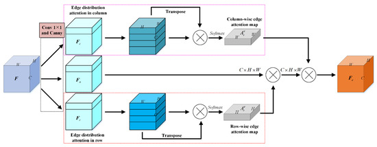
Figure 3.
Pipeline of EDA.
For row-wise, the input feature map is split in channel dimension as . As discussed in Section 2.2 and Section 3.2.1, we define and formulate edge covariance matrix as follows:
where is an average matrix and . The is re-defined row-wise edge covariance matrix. The subscript denotes the row and superscript means edge respectively. In addition, superscript is the transpose of matrix. Therefore, the row-wise edge attention map is generated followed by a Softmax layer,
where represents position in . Intuitively, the quantifies the correlations between row and row and . Afterward, the depth-wise right matrix multiplication is applied to augment the feature map as , where represents the feature map of channel.
As to column-wise edge attention pipeline, the similar calculations are implemented. First of all, the is split in channel dimension. In addition, the following matrix is defined,
where means the channel in and also represents the average values. Then, the column-wise correlations can be produced,
where represents position in . Intuitively, the quantifies the correlations between column and column and . Subsequently, a depthwise left matrix multiplication is realized. Finally, an EDA refines the input feature maps to
where subscript denotes the channels’ feature matrix and denotes the edge distribution enhanced feature maps.
3.3. Hybrid Attention Module
In Section 2.3 and Section 3.2.2, the pipeline of SAM and EDA were explained. The chapter that follows moves on to deliberate the fusion of these two modules.
Resort to the comprehensive analysis of residual connection; it is an efficient way to highlight the edge information in learnt representations. In this way, the pixels in the boundary areas have an auxiliary representation-tensor, making the error-prone pixels easily classified with high certainty and correctness. And the details are illustrated in Figure 4.
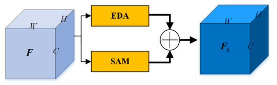
Figure 4.
Pipeline of HAM.
Formally, let the input feature maps be , where is the height, is the width and is the number of channel. Feeding the original feature map to HAM, two parallel branches form two refined feature maps, they are and respectively. In addition, both the two refined feature maps have same dimensions with . Thus, HAM generates the output feature maps,
where is the output refined feature maps by HAM, and are the learnable coefficients of weights.
Generally speaking, with the design of HAM, the edge-enhanced features are injected into position-attentive components. To further verify the importance of two kinds of features, the learnable coefficients are devised and they can be optimized along with training. Using HAM to model the dependencies of global edge distribution and position-wise dependencies over local and global areas, the learnt features can provide more reasonable and consistent semantic cues.
4. Experiments and Results
4.1. Experimental Settings
4.1.1. Datasets
Turning now to the experiments, the datasets and their properties are introduced firstly. Then, as listed in Table 1, three representative benchmarks are used to evaluate the performance. ISPRS Vaihingen and Potsdam datasets are acquired by airborne sensors with very high spatial resolution, while the DeepGlobe dataset contains satellite images from the DigitalGlobe platform. The rest of this section presents the data description in detail.

Table 1.
Datasets and properties.
- ISPRS Vaihingen dataset
The Vaihingen dataset [43] is acquired by airborne sensors that cover the Vaihingen region in Germany. Semantic labeling of the urban objects at the pixel level is challenging due to the high intra-class variance while the inter-class is low. Therefore, the semantic segmentation of very high-resolution aerial images drives extensive scholars to design advanced processing techniques. In the associated label images, six categories are annotated. They are impervious surfaces, building, low vegetation, tree, car and clutter/background.
As shown in Figure 5c,d, the raw image consists of three spectral bands: Red (R), Green (G) and Near Infrared (NIR). According to the public data, there are 16 images with a spatial size of around 2500 × 2500 available. The ground sample distance (GSD) is 9 cm.
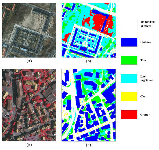
Figure 5.
Illustration of ISPRS data samples. (a) Raw image of Potsdam dataset, (b) annotated ground truth of (a), (c) raw image of Vaihingen dataset, (d) annotated ground truth of (c).
- 2.
- ISPRS Potsdam dataset
Another available semantic labeling benchmark of ISPRS is the Potsdam dataset [44], imaging on an airborne platform. The illustration of a random sample is presented in Figure 5a,b. The spatial size is 6000 × 6000 pixels with a 5 cm of GSD. The same annotations are labeled as the Vaihingen dataset. This dataset releases 24 images for academic objectives.
- 3.
- DeepGlobe dataset
DeepGlobe land cover classification dataset [45] contains high-resolution satellite images courtesy of DigitalGlobe. The available data consists of 803 images with the spatial size of 2448 × 2448. Correspondingly, the well-annotated ground truth images label seven categories. They are urban land, agriculture land, rangeland, forest land, water, barren land and unknown area. Figure 6a,c are two samples and Figure 6b,d are the associated label image.
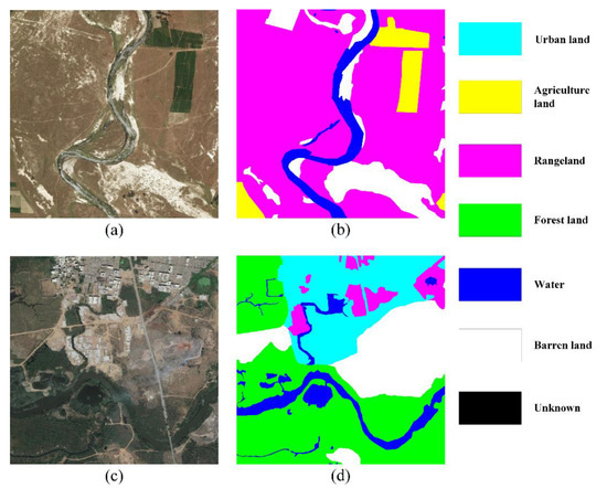
Figure 6.
Illustration of DeepGlobe data samples. (a) Raw image, (b) annotated ground truth of (a), (c) raw image, (d) annotated ground truth of (c).
Generally speaking, to extensively evaluate the performance, both aerial and satellite images are necessary to be tested. Considering the heterogeneous intra-class variants and inter-class similarities, the network is expected to learn the key information, unraveling the inherent correlations. So, ISPRS benchmarks and the DeepGlobe dataset are tested.
4.1.2. Hyper-Parameters and Implementation Details
Prior to the experiments, the hyper-parameter settings should be clearly defined and identified. As listed in Table 2, the hyper-parameters and implementation details are presented. Initially, the raw images and annotated ground truth are split to sub-patches with a spatial size of 256 × 256. Then, uniformly, the data partitioning subjects to a ratio of 8:1:1. In addition, the three parts of data is non-overlapping. The validation and test datasets are un-trained. In addition, the same data augmentations are applied.
Table 2.
Hyper-parameters and implementation details.
Moreover, the backbone, ResNet 101, is commonly used due to the less transformation loss and feature distortions by residual connections. In our network, ResNet 101 corresponds to the standard encoder in Figure 2 and the decoder is symmetric. In addition, the layers and structures are referred to [59].
As listed in Table 3, several mainstream methods, including classical segmentation networks, attention-based methods and RSI-specific networks, are compared to evaluate performance comprehensively. Some of them are initially designed for natural images, yet we re-implement these methods on three RSI datasets successfully and yield a not bad result. In contrast, no previous study has investigated the statistical edge and incorporated it in an end-to-end learnable style, causing performance bottlenecks.
Table 3.
Comparative methods.
4.1.3. Numerical Metrics
In experiments, two widely used numerical metrics, OA (Overall Accuracy) and mIoU (mean intersection over union) are calculated to quantify the performance.
where TP denotes the number of true positives, FP denotes the number of false positives, FN denotes the number of false negatives and TN denotes the number of true negatives.
4.2. Comparison with State-of-the-Art
We reasoned that the extraction and injection of edge distributions attentively performs important effects on boosting the segmentation accuracy. In our work, we sought to establish a methodology for leveraging prior edge information of learnt features. Inspired by two directional covariance matrix analysis, EDA is devised and incorporated into EDENet. To evaluate the performance, the experiments are carried on three different benchmarks. The rest of this section will further compare and discuss the collected results.
4.2.1. Results on Vaihingen Dataset
Table 4 reports results on the Vaihingen test set and highlights the best performance in bold. Apart from overall accuracy and mIoU, the class-wise accuracy and IoU are also collected in OA/IoU form for individual categories. Generally speaking, it is apparent that the highest OA and mIoU values are obtained by EDENet, demonstrating exceptionally good performance in accuracy.
Table 4.
Results on Vaihingen dataset. Accuracy of each category is presented in the OA/IoU form.
The baseline models, such as SegNet, U-Net and DeepLab V3+, are susceptible to the interference of ubiquitously subsistent intra-class variants and inter-class similarities. Among them, SegNet has an OA of 79.10%, dramatically lower than EDENet with more than ten percentages. DeepLab V3+ enlarges the receptive field to capture more local-contextual information, boosting the segmentation results by increasing about 2.5% in OA and 6% in mIoU than SegNet. However, the results are imprecise enough.
Resorting to the powerful capability in learning long-range dependencies of attention mechanisms CBAM, DANet, NLNet and OCRNet eventually corroborate the impacts of these dependencies. By the similarity analysis, also known as the generation of attention map, position-wise representations are refined with more contextual information that amplifies the margin distance of categorical representations. As a result, the geo-details are enhanced, reducing the uncertainty in identification. Compared to classical models, attention-based methods have experienced a remarkable overall improvement. The early proposed CBAM and DANet employ channel-wise attention and spatial-wise attention parallelly to enrich the contextual information, arising OA and mIoU at about 1% than DeepLab V3+. It is worth noting that CBAM and DANet have fewer parameters and time costs than DeepLab V3+. Moreover, NLNet proposed a positional self-attention mechanism, capturing channel and spatial correlations simultaneously. Therefore, the OA and mIoU further increase to more than 83% and 71%. Specifically, OCRNet even reaches more than 72% in mIoU and 85% in OA by quantifying and injecting pixel-object correlations in addition to pixel-pixel correlations.
Initially, these natural image-targeted networks are not inadequate for RSI. It is suggested that two critical properties of RSI lead to insufficient applications. One is that RSI is always acquired from a high-altitude angle. The other is the wide observation range and the covered complex and diverse visual objects by imaging sensors. For example, the visual illustration of cars is with different colors, shapes, textures, even sheltered by trees, buildings, or shadows. Striven to alleviate the interference, it is necessary to enhance the distinguishability of learnt representations. Conventionally, ResUNet-a integrates various strategies to promote the probability of correct classification, including multi-task inference, multi-residual connections, atrous convolutions, pyramid scene parsing pooling and optimized Dice loss function. Even though the accuracy, which achieves 87.25% in OA and 75.43% in mIoU, is acceptable, the size of the trained model parameter is large and the time and memory occupation are criticized. In contrast, SCAttNet is a lightweight model that uses a dual attention mechanism to optimize the learnt feature maps.
Thus far, the previous works have argued that the attention mechanism is also applicable in RSI semantic segmentation. Nevertheless, they equally handle the pixels, whether they are edge-pixel or not. As discussed in Section 1, the edge pixels are error-prone, conjointly impact the around pixels’ classification to an extent. Starting from the image covariance matrix analysis, we find that edge distributions can be learned and utilized. Then, the column-wise and row-wise edge attention maps are generated and injected into learnt representations to highlight the edge pixels. Consequently, the OA and mIoU are strikingly boosted. Compared to ResUNet-a, which has the best performance on RSI yet, EDENet increases OA and mIoU more than 2% and 1% by a few matrix manipulations. More concretely, EDENet surprisingly enhances the segmentation performance on all categories, especially in distinguishing objects with confusing features. As for cars, which are sensitive to the boundary when recognizing, the growth of accuracy is excellent, with almost 5% to ResUNet-a. Unquestionably, the exact contour enables the easily-confused pixels in short-distance and long-distance to be correctly classified with high definiteness.
The visual inspection is presented in Figure 7. We randomly select two samples and predict the pixel-wise label. Intuitively, deep neural networks are capable of applying to RSI semantic segmentation tasks. Thus, the objects are labeled corresponding to ground truth. Nonetheless, the blurry boundaries are ubiquitous by existing methods, leading to unsatisfactory results. As for easily-confused low vegetation and trees, the delineation of boundaries plays a pivotal role in locating the position of objects. With an accurate location, the segments tend to be more complete and consistent.
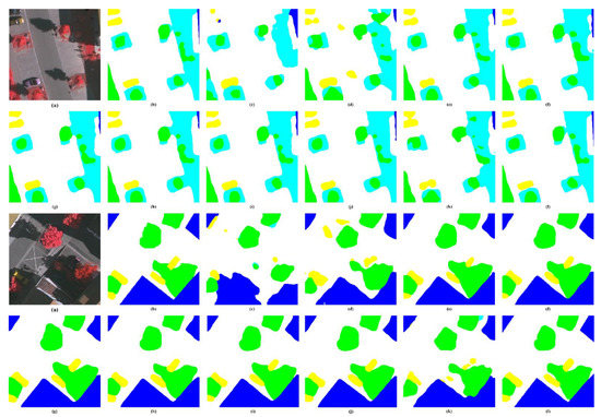
Figure 7.
Visual inspections of random samples from Vaihingen test set. (a) raw image, (b) ground truth, (c) SegNet, (d) U-Net, (e) DeepLab V3+, (f) CBAM, (g) DANet, (h) NLNet, (i) OCRNet, (j) ResUNet-a, (k) SCAttNet, (l) EDENet.
To sum up, attributing to the distinct boundaries by injecting edge distributions attentively, overall accuracy and visualizations are significantly improved compared to other SOTA methods on the ISPRS Vaihingen benchmark.
4.2.2. Results on Potsdam Dataset
Different from the Vaihingen dataset, Potsdam has more data for training and validation. Meanwhile, the ground objects exhibit entirely heterogeneous visual characteristics, as previously illustrated in Table 5.
Table 5.
Results on Potsdam dataset. Accuracy of each category is presented in the OA/IoU form.
Coincidentally, the overall accuracy performs similar trends to Vaihingen. In addition, the OA and mIoU are relatively higher than Vaihingen by EDENet. Furthermore, all the category-wise accuracy of EDENet is also the highest to other models. This fact suggests that EDENet manifests decent generalizability. Moreover, owing to the abundant well-annotated data for training, the robustness of the network is enhanced.
In general, attention-based methods are feasible for capturing various contextual information, facilitating the learning ability of geo-objects. Therefore, the accuracy of attention-based methods is holistically superior to the classical ones. Above all, OCRNet takes advantage of pixel-object contextual relationships besides pixel-wise relationships, revealing the significance of geo-objects’ representations. In this way, OCRNet reaches more than 85% of overall accuracy and 72% of mIoU, dramatically improving. Similarly, SCAttNet designed dual attention modules to answer the complex of RSI objects, resulting in almost the same level of performance to OCRNet. By combining multiple tricks, ResUNet-a boosts the overall accuracy of 2% than OCRNet.
However, the existing methods are still far from EDENet, which produces a very competitive result. Specifically, the impervious surfaces and buildings are barely misclassified. Moreover, the easy-confused low vegetation and trees are also duly partitioned by the prior knowledge of edge. In addition, the classification of cars depends on locating the position, which is closely related to the edge information. Eventually, cars have the most considerable growth.
For qualitative evaluation, two samples of the Potsdam test set are predicted and illustrated in Figure 8. Sharpen edges make the interior pixels of an object more accessible to be classified correctly. For instance, the low vegetation and trees always appear concurrence a neighboring. However, from the visual perspective in RSI, they are easily-confused by the high inter-class consistency. Once the boundaries are misregistered, a deluge of pixels is forced to be wrongly predicted. Although attention-based and RSI-specific approaches have leveraged contextual information to enhance the distinguishability between different categories’ pixels, the blurry edges still trouble the semantic segmentation performance. As we can see, cars, marked as yellow, are challenging to outline under deficient boundaries wholly. Figure 8l shows the results produced by EDENet, by which the edges are retained to the uttermost refers to ground truth. In fact, EDENet segments RSI with high-fidelity and high consistency.
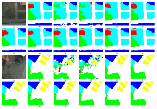
Figure 8.
Visual inspections of random samples from Potsdam test set. (a) raw image, (b) ground truth, (c) SegNet, (d) U-Net, (e) DeepLab V3+, (f) CBAM, (g) DANet, (h) NLNet, (i) OCRNet, (j) ResUNet-a, (k) SCAttNet, (l) EDENet.
Overall, EDENet expresses strong power in applying to RSI with different spatial resolution and various ground features according to the quantitative and qualitative evaluations. The exceptionally preferable results are obtained by learning and injecting edge distributions of feature maps, which indirectly help the network adjust error-prone pixels.
4.2.3. Results on DeepGlobe Dataset
As discussed above, the DeepGlobe dataset collects high-resolution sub-meter satellite imagery. Due to the variety of land cover types and the density of annotations, this dataset is more challenging than existing counterparts like ISPRS benchmarks. In this regard, the grade of difficulty in semantic segmentation is leveled up majorly.
As reported in Table 6, the quantitative results are collected, where the bold number indicates the best. Typically, the OA and mIoU have appreciably decrease compared to ISPRS benchmarks, ascribing to the indistinguishable spatial and spectral features by satellite sensors. Still and all, EDENet realizes the accurate classification of each category without exception, contributing to the highest OA and mIoU of more than 83% and 60%, respectively. To our knowledge, the differential accuracy across all categories is accounted for the imbalanced distribution, among which the agricultural land has the most pixels.
Table 6.
Results on DeepGlobe dataset. Accuracy of each category is presented in the OA/IoU form.
Comparing classical and attention-based ones has convinced the achievability and availability of attention mechanisms in RSI feature optimization. CBAM, DANet and NLNet extract global context by attention modules to enrich the inference cues and a fair increase of more than 1% than DeepLab V3+ is produced. With more complementary contextual information, OCRNet further boosts OA by about 1%. Likewise, SCAttNet sequentially embeds channel and spatial attention modules to refine the learnt features adaptively. As a result, this lightweight network achieves similar performance to OCRNet. Empirically, ResUNet-a analyzes the essence of RSI when distinct confusable pixels and employs multiple manipulations. Therefore, the OA and mIoU are over 80% and 58% by ResUNet-a, which is the first place ever before. Unfortunately, these models ignore the impacts of localization by edge delineation, triggering rough boundaries. EDENet learns the edge distributions and injects them into feature optimization, provoking a significant improvement of accuracy.
In the visual inspections from Figure 9, the top sample covers five classes of ground. Inherently, the water areas surrounding rangeland and agricultural land are not visually recognizable. In addition, the classical networks work poorly on distinct these objects. In this context, consistent boundaries are critical in actuating the network to separate the different pixels assuredly. EDENet keeps the highest consistency with ground truth by highlighting the edges in learnt representations compared to the SOTA methods. Similar to the bottom sample, only a tiny part of the edges is out of position, leading to some blurry boundary and misclassification bias. However, the global accuracy and consistency are retained.
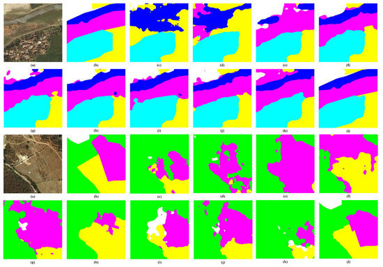
Figure 9.
Visual inspections of random samples from DeepGlobe test set. (a) raw image, (b) ground truth, (c) SegNet, (d) U-Net, (e) DeepLab V3+, (f) CBAM, (g) DANet, (h) NLNet, (i) OCRNet, (j) ResUNet-a, (k) SCAttNet, (l) EDENet.
To sum up, EDENet can adaptively learn and highlights the edges without depending on the spatial resolution or the visual separability. Although the overall accuracy is decreased, EDENet outperforms SOTA methods remarkably. In addition, the achievements further demonstrate the strong generalizability of EDENet on multi-sensors imagery.
4.3. Ablation Study of EDA
The previous studies using CNNs indicate that learning distinguishable representations is essential to enhance segmentation performance. Furthermore, attention mechanisms are employed as an efficient way to refine representations. Nevertheless, they did not learn the edge information, which is pivotal to localize the objects and calibrate the pixels around the edge. The devised EDA bridges this gap by attentively learning prior edge distribution in feature maps at arbitrary scales. In addition, we heliacally embed this module to standard encoder-decoder architecture, generating excellent results.
To comprehensively evaluate EDA, the ablation study is implemented under the same hyper-parameters and runtime environment. Practically, a version that removes the EDA from HAM in Figure 4 is constructed and named as non-EDA. Now, as presented in Table 7, the OA and mIoU are collected to analyze the effects. Generally, EDA elicits about a 5% increase on Vaihingen and Potsdam datasets in OA and 4% on DeepGlobe. As for mIoU, the relative improvements are deserved. The effects of EDA are dramatically illustrated. Moreover, we monitor the loss and mIoU during the training process to support the evaluation, which can be seen in appendices.
Table 7.
Ablation study’s results. The accuracy is presented in the OA/mIoU form.
Overall, EDA essentially guarantees unbiased edges, resulting in visually well-segmented objects and obtaining desirable quantitative accuracy.
5. Discussions
Prior studies have noted the importance of contextual information in enhancing the distinguishability of learnt representations. Attention mechanisms paved an effective way for capturing the context by several matrix manipulations. Thus, the accuracy has been boosted. However, the edges should be emphasized due to their essential locations. Once the edges are failed to be delineated, the blurs will lead to misconceived and omissive pixels. Therefore, our study seeks to produce a new attention module, which can be flexibly embedded into the end-to-end segmentation network and a learnable way to extract and inject edge distributions of learnt feature maps.
Inspired by the attention mechanism and covariance matrix analysis in 2DPCA, we propose EDENet, which hierarchically embeds hybrid attention modules that learns convolved features and highlights edge distributions simultaneously. As a result, the experiments on aerial and satellite images have illustrated the excellence of EDENet. Both numerical evaluations and visual inspections have supported this finding. Moreover, unlike SOTA RSI-specific methods, the OA and mIoU are improved significantly without the complex design of network architecture.
6. Conclusions
The semantic segmentation of RSI plays a pivotal role for various downstream applications. In addition, boosting the accuracy of segmentation has been a hot topic in the field. The existing approaches have produced competitive results by attention-based deep convolutional neural networks. However, the deficiency of edge information leads to blurry boundaries, even raising high uncertainties of long-distant pixels during recognition.
In this study, we have investigated an end-to-end trainable semantic segmentation neural network of RSI. Essentially, we first formulate and model the edge distributions of encoded feature maps inspired by covariance matrix analysis. Then, the designed EDA learns the column-wise and row-wise edge attention maps in a self-attentive fashion. As a result, the edge knowledge is successfully modeled and injected into learnt representations, facilitating representativeness and distinguishability. In addition to leverage edge distributions, HAM employs non-local block as another parallel branch to capture the position-wise dependencies. As a result, the complementary contextual and edge information are learned to enhance the discriminative capability of the network. In experiments, three diverse datasets from multiple sensors and different imaging platforms are examined. The results indicate the efficacy and superiority of the proposed model. With the ablation study, we further demonstrate the effects of EDA.
Nevertheless, there are still several challenging issues to be addressed. First of all, the multi-modal data are necessarily fused to improve the semantic segmentation performance, such as DSM information and SAR data. Moreover, the transferable models are of great concern to adaptively cope with the increasingly diverse imaging sensors. Furthermore, the basic convolution units also have the potential to be optimized in convergence rate while producing a global-optimal solution, as the previous work has validated [60]. In addition, the semantic segmentation tasks, image fusion [61], image denoising [62] and image restoration [63] of remote sensing images also rely on the feature extraction; the extension of the proposed module should be promising and challenging.
Author Contributions
Conceptualization, X.L. and R.X.; methodology, X.L. and Z.C.; software, Z.C.; validation, X.L., T.L. and R.X.; formal analysis, X.L.; investigation, R.X.; resources, X.L. and Z.C.; data curation, K.Z. and Z.C.; writing—original draft preparation, X.L.; writing—review and editing, T.L. and R.X.; visualization, X.L.; supervision, R.X.; project administration, T.L. and R.X.; funding acquisition, R.X. Besides, T.L. and R.X. have equal contributions. All authors have read and agreed to the published version of the manuscript.
Funding
The study was financially supported by the National Key Research and Development Program (Grant No. 2018YFC0407905), the Science Fund for Distinguished Young Scholars of Henan Province (Grant No. 202300410539), the Science Fund for Excellent Young Scholars of Henan Province (Grant No. 212300410059), the Major scientific and technological special project of Henan Province (Grant No. 201400211000), the National Natural Science Fund of China (Grant No. 51779100 and 51679103), Central Public-interest Scientific Institution Basal Research Fund (Grant No. HKY-JBYW-2020-21 and HKY-JBYW-2020-07).
Institutional Review Board Statement
Not applicable.
Informed Consent Statement
Not applicable.
Data Availability Statement
Publicly available datasets were analyzed in this study. The data can be found here: [https://www2.isprs.org/commissions/comm2/wg4/benchmark/semantic-labeling/] and [http://deepglobe.org/] (Accessed on 10 December 2021).
Conflicts of Interest
The authors declare no conflict of interest.
Appendix A. Ablation Study on the Vaihingen Dataset
As outlined in the previous discussions, the test aims to evaluate the efficacy and superiority of EDA. Under the constant environment and hyper-parameter settings, we implement the no-EDA version on the Vaihingen dataset and record the loss and mIoU during the training process.
As illustrated in Figure A1, the training loss is drawn. Embedding EDA makes the network convergence with a lower training loss (cross-entropy loss). Furthermore, EDENet drops the loss from 0.1850 to 0.0409 compared to no-EDA version. Correspondingly, the mIoU given in Figure A2 reveals the tremendous changes. EDENet reaches up to 95.51% on mIoU, while no-EDA version merely has 84.03%.
On the whole, we found evidence to suggest that edges may be closely related to contribute to calibrate the error-prone pixels around boundaries. From this perspective, injecting and underlining the edge distributions of leant representations plays a crucial role in sharpening the segments.
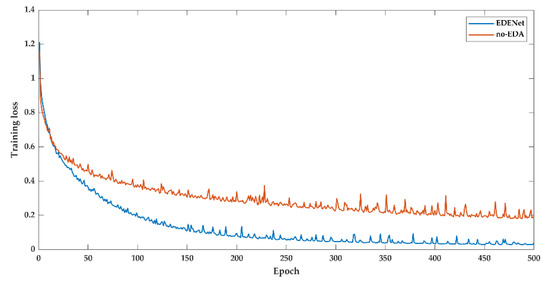
Figure A1.
Training loss of Vaihingen dataset.
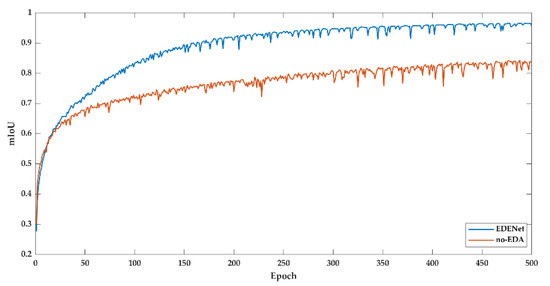
Figure A2.
Training mIoU of Vaihingen dataset.
Appendix B. Ablation Study on the Potsdam Dataset
For the Potsdam dataset, the loss and mIoU during the training process are also compared. As shown in Figure A3 and Figure A4, the curves are presented. The variation of spatial resolution and objects’ visual sensitivity is incapable of degrading the performance of EDENet. EDA decreases a great deal of training loss. Numerically, the loss is dropped from 0.2199 to 0.0503 over 77%. Turn to mIoU, EDA boosts the result from 82.89% to 94.81%.
In general, the recorded results on the Potsdam dataset follow similar patterns to the Vaihingen dataset.
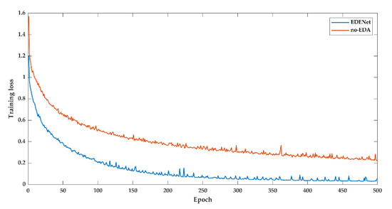
Figure A3.
Training loss of Potsdam dataset.
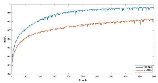
Figure A4.
Training mIoU of Potsdam dataset.
Appendix C. Ablation Study on the DeepGlobe Dataset
DeepGlobe dataset consists of a deluge of satellite images showing diverse and complex land cover types. Figure A5 and Figure A6 plot the training loss and mIoU changing status. There is a lower loss along with the training phase of EDENet. It eventually drops the loss from 0.2625 to 0.1461 at the 200 epoch. Accordingly, the mIoU experiences a considerable improvement of about 12%.
Another observation lies in the variation tendency, which still retains a declining status of EDENet at the 200 epoch, while no-EDA version is almost going to converge. This phenomenon substantially gives rise to the potentials of EDENet. Therefore, with more epochs of training, we are convinced of achieving great promotion
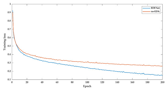
Figure A5.
Training loss of DeepGlobe dataset.
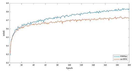
Figure A6.
Training mIoU of DeepGlobe dataset.
References
- Xia, M.; Cui, Y.; Zhang, Y.; Xu, Y.; Xu, Y. DAU-Net: A novel water areas segmentation structure for remote sensing image. Int. J. Remote Sens. 2021, 42, 2594–2621. [Google Scholar] [CrossRef]
- Weng, L.; Xu, Y.; Xia, M.; Zhang, Y.; Xu, Y. Water areas segmentation from remote sensing images using a separable Residual SegNet network. ISPRS Int. J. Geo-Inf. 2020, 9, 256. [Google Scholar] [CrossRef]
- Yang, Q.; Liu, M.; Zhang, Z.; Yang, S.; Ning, J.; Han, W. Mapping Plastic mulched farmland for high resolution images of unmanned aerial vehicle using deep semantic segmentation. Remote Sens. 2019, 11, 2008. [Google Scholar] [CrossRef] [Green Version]
- Tong, X.; Xia, G.; Lu, Q.; Shen, H.; Li, S.; You, S.; Zhang, L. Land-cover classification with high-resolution remote sensing images using transferable deep models. Remote Sens. Environ. 2020, 237, 11132. [Google Scholar] [CrossRef] [Green Version]
- Henry, C.J.; Storie, C.D.; Palaniappan, M.; Alhassan, V.; Swamy, M.; Aleshinloye, D.; Curtis, A.; Kim, D. Automated LULC map production using deep neural networks. Int. J. Remote Sens. 2019, 40, 4416–4440. [Google Scholar] [CrossRef]
- Shi, H.; Chen, L.; Bi, F.; Chen, H.; Yu, Y. Accurate urban area detection in remote sensing images. IEEE Geosci. Remote Sens. Lett. 2015, 12, 1948–1952. [Google Scholar] [CrossRef]
- Wegner, J.D.; Branson, S.; Hall, D.; Schindler, K.; Perona, P. Cataloging public objects using aerial and street-level images-Urban trees. In Proceedings of the 29th IEEE Computer Society Conference on Computer Vision and Pattern Recognition (CVPR), Las Vegas, NV, USA, 26 June–1 July 2016; pp. 6014–6023. [Google Scholar]
- Ozdarici, A.; Schindler, K. Mapping of agricultural crops from single high-resolution multispectral images data-driven smoothing vs. parcel-based smoothing. Remote Sens. 2015, 7, 5611–5638. [Google Scholar] [CrossRef] [Green Version]
- Gibril, M.B.A.; Shafri, H.Z.M.; Shanableh, A.; Al-Ruzouq, R.; Wayayok, A.; Hashim, S.J. Deep convolutional neural network for large-scale date palm tree mapping from UAV-based images. Remote Sens. 2021, 13, 2787. [Google Scholar] [CrossRef]
- Minaee, S.; Boykov, Y.; Porikli, F.; Plaza, A.J.; Kehtarnavaz, N.; Terzopoulos, D. Image segmentation using deep learning: A survey. IEEE Trans. Pattern Anal. Mach. Intell. 2021. accepted. [Google Scholar] [CrossRef]
- Arivazhagan, S.; Ganesan, L.; Priyal, S. Texture classification using Gabor wavelets based rotation invariant features. Pattern Recognit. Lett. 2006, 27, 1976–1985. [Google Scholar] [CrossRef]
- Gitelson, A.; Merzlyak, M. Signature analysis of leaf reflectance spectra: Algorithm development for remote sensing of chlorophyll. J. Plant Physiol. 1996, 148, 494–500. [Google Scholar] [CrossRef]
- Peñ, A.; José, M.; Ngugi, M.; Richard, E.P.; Johan, S. Object-based crop identification using multiple vegetation indices, textural features and crop phenology. Remote Sens. Environ. 2011, 115, 1301–1316. [Google Scholar]
- Blaschke, T. Object based image analysis for remote sensing. ISPRS J. Photogramm. Remote Sens. 2010, 65, 2–16. [Google Scholar] [CrossRef] [Green Version]
- Yang, J.; Jiang, Z.; Zhou, Q. Remote sensing image semantic labeling based on conditional random field. Acta Aeronaut. Astronaut. Sin. 2015, 36, 3069–3081. [Google Scholar]
- Mountrakis, G.; Im, J.; Ogole, C. Support vector machines in remote sensing: A review. ISPRS J. Photogramm. Remote Sens. 2011, 66, 247–259. [Google Scholar] [CrossRef]
- Belgiu, M.; Lucian, D. Random forest in remote sensing: A review of applications and future directions. ISPRS J. Photogramm. Remote Sens. 2016, 114, 24–31. [Google Scholar] [CrossRef]
- Long, J.; Shelhamer, E.; Darrell, T. Fully convolutional networks for semantic segmentation. IEEE Trans. Pattern Anal. Mach. Intell. 2015, 39, 640–651. [Google Scholar]
- Badrinarayanan, V.; Kendall, A.; Cipolla, R. SegNet: A deep convolutional encoder-decoder architecture for image segmentation. IEEE Trans. Pattern Anal. Mach. Intell. 2017, 39, 2481–2495. [Google Scholar] [CrossRef] [PubMed]
- Ronneberger, O.; Fischer, P.; Brox, T. U-Net: Convolutional networks for biomedical image segmentation. In Proceedings of the Medical Image Computing and Computer-Assisted Intervention (MCCAI), Munich, Germany, 5–9 October 2015; Volume 9351, pp. 234–241. [Google Scholar]
- Chen, L.; Papandreou, G.; Kokkinos, L.; Murphy, K.; Yuille, A. Semantic image segmentation with deep convolutional nets and fully connected CRFs. In Proceedings of the 3rd International Conference on Learning Representations (ICLR), San Diego, CA, USA, 7–9 May 2015. [Google Scholar]
- Chen, L.; Papandreou, G.; Kokkinos, I.; Murphy, K.; Yuille, A. DeepLab: Semantic image segmentation with deep convolutional nets, atrous convolution, and fully connected CRFs. IEEE Trans. Pattern Anal. Mach. Intell. 2018, 40, 834–848. [Google Scholar] [CrossRef] [PubMed]
- Chen, L.; Papandreou, G.; Schroff, F.; et al. Rethinking atrous convolution for semantic image segmentation. arXiv 2017, arXiv:1706.05587. [Google Scholar]
- Chen, L.; Zhu, Y.; Papandreou, G.; Adam, H. Encoder-decoder with atrous separable convolution for semantic image segmentation. In Proceedings of the 15th European Conference on Computer Vision (ECCV), Munich, Germany, 8–14 September 2018; pp. 833–851. [Google Scholar]
- Zhang, J.; Lin, S.; Ding, L.; Bruzzone, L. Multi-scale context aggregation for semantic segmentation of remote sensing images. Remote Sens. 2020, 12, 701. [Google Scholar] [CrossRef] [Green Version]
- Sun, K.; Xiao, B.; Liu, D.; Wang, J. Deep high-resolution representation learning for human pose estimation. In Proceedings of the 32nd IEEE Computer Society Conference on Computer Vision and Pattern Recognition (CVPR), Long Beach, CA, USA, 16–20 June 2019; pp. 5686–5696. [Google Scholar]
- Chen, B.; Xia, M.; Huang, J. MFANet: A multi-level feature aggregation network for semantic segmentation of land cover. Remote Sens. 2021, 13, 731. [Google Scholar] [CrossRef]
- Wang, E.; Jiang, Y. MFCSNet: Multi-scale deep features fusion and cost-sensitive loss function based segmentation network for remote sensing images. Appl. Sci. 2019, 9, 4043. [Google Scholar] [CrossRef] [Green Version]
- Hu, J.; Shen, L.; Albanie, S.; Sun, G.; Wu, E. Squeeze-and-excitation networks. IEEE Trans. Pattern Anal. Mach. Intell. 2020, 42, 2011–2023. [Google Scholar] [CrossRef] [Green Version]
- Woo, S.; Park, J.; Lee, J.; Kweon, I. CBAM: Convolutional block attention module. In Proceedings of the 15th European Conference on Computer Vision (ECCV), Munich, Germany, 8–14 September 2018; pp. 3–19. [Google Scholar]
- Fu, J.; Liu, J.; Tian, H.; Li, Y.; Bao, Y.; Fang, Z.; Lu, H. Dual attention network for scene segmentation. In Proceedings of the 32nd IEEE/CVF Conference on Computer Vision and Pattern Recognition (CVPR), Long Beach, CA, USA, 16–20 June 2019; pp. 3141–3149. [Google Scholar]
- Wang, X.; Girshick, R.; Gupta, A.; He, K. Non-local neural networks. In Proceedings of the 31st Conference on Computer Vision and Pattern Recognition (CVPR), Salt Lake City, UT, USA, 18–22 June 2018; pp. 7794–7803. [Google Scholar]
- Zhang, F.; Chen, Y.; Li, Z.; Hong, Z.; Ding, E. ACFNet: Attentional class feature network for semantic segmentation. In Proceedings of the 17th IEEE International Conference on Computer Vision (ICCV), Seoul, Korea, 27 October–2 November 2019; pp. 6797–6806. [Google Scholar]
- Yuan, Y.; Chen, X.; Wang, J. Object-contextual representations for Semantic Segmentation. In Proceedings of the 16th European Conference on Computer Vision (ECCV), 23–28 August 2020; pp. 173–190. [Google Scholar]
- Ghaffarian, S.; Valente, J.; Voort, M.; Tekinerdogan, B. Effect of attention mechanism in deep learning-based remote sensing image processing: A systematic literature review. Remote Sens. 2021, 13, 2965. [Google Scholar] [CrossRef]
- Luo, H.; Chen, C.; Fang, L.; Zhu, X.; Lu, L. High-resolution aerial images semantic segmentation using deep fully convolutional network with channel attention mechanism. IEEE J. Sel. Top. Appl. Earth Obs. Remote Sens. 2019, 12, 3492–3507. [Google Scholar] [CrossRef]
- Niu, R.; Sun, X.; Tian, Y.; Diao, W.; Chen, K.; Fu, K. Hybrid multiple attention network for semantic segmentation in aerial images. IEEE Trans. Geosci. Remote Sens. 2021. accepted. [Google Scholar] [CrossRef]
- Li, H.; Qiu, K.; Chen, L.; Mei, X.; Hong, L.; Tao, C. SCAttNet: Semantic segmentation network with spatial and channel attention mechanism for high-resolution remote sensing images. IEEE Geosci. Remote Sens. Lett. 2021, 18, 905–909. [Google Scholar] [CrossRef]
- Ding, L.; Tang, H.; Bruzzone, L. LANet: Local attention embedding to improve the semantic segmentation of remote sensing images. IEEE Trans. Geosci. Remote Sens. 2020. accepted. [Google Scholar] [CrossRef]
- Marmanis, D.; Schindler, K.; Wegner, J.; Galliani, S.; Datcu, M.; Stilla, U. Classification with an edge: Improving semantic image segmentation with boundary detection. ISPRS J. Photogramm. Remote Sens. 2018, 135, 158–172. [Google Scholar] [CrossRef] [Green Version]
- Pan, S.; Tao, Y.; Nie, C.; Chong, Y. PEGNet: Progressive edge guidance network for semantic segmentation of remote sensing images. IEEE Geosci. Remote Sens. Lett. 2021, 18, 637–641. [Google Scholar] [CrossRef]
- Yang, J.; Zhang, D.; Frangi, A.; Yang, J. Two-dimensional PCA: A new approach to appearance-based face representation and recognition. IEEE Trans. Pattern Anal. Mach. Intell. 2004, 26, 131–137. [Google Scholar] [CrossRef] [Green Version]
- ISPRS Vaihingen 2D Semantic Labeling Dataset. Available online: http://www2.isprs.org/commissions/comm3/wg4/2d-sem-label-vaihingen.html (accessed on 10 December 2017).
- ISPRS Potsdam 2D Semantic Labeling Dataset. Available online: http://www2.isprs.org/commissions/comm3/wg4/2d-sem-label-potsdam.html (accessed on 10 December 2017).
- Ilke, D.; et al. DeepGlobe 2018: A challenge to parse the Earth through satellite images. In Proceedings of the 31th IEEE/CVF Conference on Computer Vision and Pattern Recognition Workshops (CVPRW), Salt Lake City, UT, USA, 18–22 June 2018; pp. 172–181. [Google Scholar]
- Vaswani, A.; Shazeer, N.; Parmar, N.; Uszkoreit, J.; Jones, L.; Gomez, A.; Kaiser, L.; Polosukhin, I. Attention is all you need. In Proceedings of the 31st Annual Conference on Neural Information Processing Systems (NIPS), Long Beach, CA, USA, 4–9 December 2017; pp. 5999–6009. [Google Scholar]
- Wei, J.; He, J.; Zhou, Y.; Chen, K.; Tang, Z.; Xiong, Z. Enhanced object detection with deep convolutional neural networks for advanced driving assistance. IEEE Trans. Intell. Transp. Syst. 2020, 21, 1572–1583. [Google Scholar] [CrossRef] [Green Version]
- Techimann, M.; Weber, M.; Zollnr, M.; Cipolla, R.; Urtasun, R. MultiNet: Real-time joint semantic reasoning for autonomous driving. In Proceedings of the 2018 IEEE Intelligent Vehicles Symposium (IV), Changshu, China, 26–30 June 2018. [Google Scholar]
- Haut, J.; Fernandez-Beltran, R.; Paolett, M.; Plaza, J.; Plaza, A. Remote sensing image super-resolution using deep residual channel attention. IEEE Trans. Geosci. Remote Sens. 2019, 57, 9277–9289. [Google Scholar] [CrossRef]
- Li, H.; Liu, Y.; Ouyang, W.; Wang, X. Zoom out-and-in network with map attention decision for region proposal and object detection. Int. J. Comput. Vis. 2019, 127, 225–238. [Google Scholar] [CrossRef] [Green Version]
- Liu, S.; Johns, E.; Davison, A. End-to-End Multi-Task Learning with Attention. arXiv arXiv:1803.10704, 2019.
- Maninis, K.; Radosavovic, I.; Kokkinos, I. Attentive single-tasking of multiple tasks. In Proceedings of the 32nd IEEE Computer Society Conference on Computer Vision and Pattern Recognition (CVPR), Long Beach, CA, USA, 16–20 June 2019; pp. 1851–1860. [Google Scholar]
- Huang, Z.; Wang, X.; Huang, L.; Huang, C.; Wei, Y.; Liu, W. CCNet: Criss-cross attention for semantic segmentation. In Proceedings of the 17th IEEE International Conference on Computer Vision (ICCV), Seoul, Korea, 27 October–2 November 2019; pp. 603–612. [Google Scholar]
- Yang, Z.; He, X.; Gao, J.; Deng, L.; Smola, A. Stacked attention networks for image question answering. In Proceedings of the 29th IEEE Computer Society Conference on Computer Vision and Pattern Recognition (CVPR), Las Vegas, NV, USA, 26 June–1 July 2016; pp. 21–29. [Google Scholar]
- Li, H.; Xiong, P.; An, J.; Wang, L. Pyramid attention network for semantic segmentation. In Proceedings of the 29th British Machine Vision Conference (BMVC), Newcastle, UK, 3–6 September 2018. [Google Scholar]
- Zhu, L.; Wang, T.; Aksu, E.; Kamarainen, J. Cross-granularity attention network for semantic segmentation. In Proceedings of the 17th IEEE/CVF International Conference on Computer Vision Workshop (ICCVW), Seoul, Korea, 27–28 October 2019; pp. 1920–1930. [Google Scholar]
- Yang, J.; Yang, J. From image vector to matrix: A straightforward image projection technique—IMPCA vs. PCA. Pattern Recognit. 2002, 35, 1997–1999. [Google Scholar] [CrossRef]
- Foivos, D.; François, W.; Peter, C.; Wu, C. ResUNet-a: A deep learning framework for semantic segmentation of remotely sensed data. ISPRS J. Photogramm. Remote Sens. 2020, 162, 94–114. [Google Scholar]
- He, K.; Zhang, X.; Ren, S.; Sun, J. Deep residual learning for image recognition. In Proceedings of the 29th IEEE Computer Society Conference on Computer Vision and Pattern Recognition (CVPR), Las Vegas, NV, USA, 26 June–1 July 2016; pp. 770–778. [Google Scholar]
- Ganguly, S. Multi-objective distributed generation penetration planning with load model using particle swarm optimization. Decis. Mak. Appl. Manag. Eng. 2020, 3, 30–42. [Google Scholar] [CrossRef]
- Xie, Q.; Zhou, M.; Zhao, Q.; Meng, D.; Zuo, W.; Xu, Z. Multispectral and hyperspectral image fusion by MS/HS fusion net. In Proceedings of the 32nd IEEE Computer Society Conference on Computer Vision and Pattern Recognition (CVPR), Long Beach, CA, USA, 16–20 June 2019. [Google Scholar]
- Chen, Y.; Huang, T.; He, W.; Zhao, X.; Zhang, H.; Zeng, J. Hyperspectral image denoising using factor group sparsity-regularized nonconvex low-rank approximation. IEEE Trans. Geosci. Remote Sens. 2021, 1–16. [Google Scholar] [CrossRef]
- He, W.; Yao, Q.; Li, C.; Yokoya, N.; Zhao, Q.; Zhang, H.; Zhang, L. Non-local meets global: An integrated paradigm for hyperspectral image restoration. IEEE Trans. Pattern Anal. Mach. Intell. 2020, 1. [Google Scholar] [CrossRef] [PubMed]
Publisher’s Note: MDPI stays neutral with regard to jurisdictional claims in published maps and institutional affiliations. |
© 2021 by the authors. Licensee MDPI, Basel, Switzerland. This article is an open access article distributed under the terms and conditions of the Creative Commons Attribution (CC BY) license (https://creativecommons.org/licenses/by/4.0/).