Sequence Image Datasets Construction via Deep Convolution Networks

Abstract

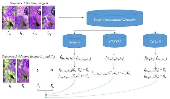
Remote-sensing time-series datasets are significant for global change research and a better understanding of the Earth. However, remote-sensing acquisitions often provide sparse time series due to sensor resolution limitations and environmental factors such as cloud noise for optical data. Image transformation is the method that is often used to deal with this issue. This paper considers the deep convolution networks to learn the complex mapping between sequence images, called adaptive filter generation network (AdaFG), convolution long short-term memory network (CLSTM), and cycle-consistent generative adversarial network (CyGAN) for construction of sequence image datasets. AdaFG network uses a separable 1D convolution kernel instead of 2D kernels to capture the spatial characteristics of input sequence images and then is trained end-to-end using sequence images. CLSTM network can map between different images using the state information of multiple time-series images. CyGAN network can map an image from a source domain to a target domain without additional information. Our experiments, which were performed with unmanned aerial vehicle (UAV) and Landsat-8 datasets, show that the deep convolution networks are effective to produce high-quality time-series image datasets, and the data-driven deep convolution networks can better simulate complex and diverse nonlinear data information.

1. Introduction

Remote-sensing time-series datasets are an important product and can be applied to research and applications in global changes, such as vegetation phenology changes, land degradation, etc. The successful application of remote-sensing time-series datasets are significant for earth science to expand the growth to a deeper level and to better understand the Earth [1,2].

Time-series analysis usually requires the data to be dense and has equal time intervals to facilitate the process. However, remote-sensing acquisitions often provide sparse time series due to sensor resolution limitations and environmental factors [3], such as cloud noise for optical data. In this case, it is difficult to conduct time-series analysis and construct remote-sensing sequence image datasets.

A conventional method to solve missing data is a linear fitting method, and only uses 1D data for transformation. Seaquist et al. [4] used the ordinary kriging (OK) method to improve the accuracy of a normalized difference vegetable index (NDVI). Berterretche et al. [5] used a spatial interpolation method to interpolate leaf-area index (LAI) data. Bhattacharjee et al. [6] compared the accuracy of remote-sensing data using different spatial interpolation methods and concluded that the accuracy of OK was better than inverse distance weight (IDW). The above methods can use the spatial information of remote-sensing images for spatial transformation, and cannot use temporal information of remote-sensing images for temporal transformation.

Zhou et al. [7] used NDVI data of moderate-resolution imaging spectroradiometer (MODIS) satellite to conduct simulation experiments and evaluate the Savitzky–Golay (SG) filtering [8] and harmonic analysis of time-series (HANTS) model [9] refactoring effect at different time intervals. According to the daily harmonic changes of land surface temperature (LST), Crosson et al. [10] used the LST data of MODIS Terra and Aqua to repair missing LST points by harmonic analysis. The above methods provide better 1D data fitting for the construction of time-series data at different time intervals and are not suitable for the transformation of high-dimensional time-series data.

The emergence of the enhanced spatial and temporal adaptive reflectance fusion model (ESTARTFM) [11], spatial and temporal adaptive reflectance fusion model (STARTFM) [12], a virtual image pair-based spatio-temporal fusion (VIPSTF) [13], and global dense feature fusion convolutional network [14] had provided ideas for research on sequence construction. These models can obtain high spatio-temporal resolution fusion data, but they cannot elaborate on the spatio-temporal evolution of sequence images and rely heavily on the situation of the original data itself.

Remote-sensing sequence images are a kind of short-range complex and nonlinear 2D data [15], and spatio-temporal information must be considered during construction. It is difficult to construct 2D images in the same way that construction is applied to 1D data. It is difficult to use the conventional linear fitting method for construction. The deep learning method can better simulate complex and diverse nonlinear data information, so it is a better choice for time-series image transformation.

Yuval et al. [16] presented benthic mapping and accelerated segmentation through photogrammetry and multi-level superpixels, and showed the accuracy of repeated surveys using orthorectification and sparse label augmentation. This approach is appropriate for any person who is interested in using photogrammetry for ecological surveys, especially diver-based underwater surveys. Kalajdjieski et al. [17] proposed a novel approach evaluating four different architectures that utilize camera images to estimate the air pollution in those areas. These images were further enhanced with weather data to boost the classification accuracy. The proposed approach exploits the deep learning method combined with data augmentation techniques to mitigate the class imbalance problem. In principle, this approach is suitable for every application where image data is correlated with sensor data, and using them in combination can be beneficial for the learning task. In particular, the adoption of this method in multi-class classification settings with imbalanced classes is particularly beneficial. Wang et al. [18] proposed an unsupervised data augmentation and effective spectral structure extraction method for all hyperspectral samples. This method not only improves the classification accuracy greatly with the newly added training samples but also further improves the classification accuracy of the classifier by optimizing the augmented testing samples. However, as discussed previously, these data augmentation methods cannot make full use of the spatio-temporal features of the original data, and the transfer learning ability of its mapping model is weak. So these methods are not well-suited for remote-sensing time-series data transformation.

Long et al. [19] used frame interpolation as a supervision signal to learn the Convolutional Neural Network (CNN) models for optical flow. However, their main target is optical flow and the interpolated frames tend to be blurry. Liu et al. [20] developed a CNN model for frame interpolation that had an explicit sub-network for motion estimation. Their method obtains not only good interpolation results but also promising unsupervised flow estimation results on KITTI 2012. Niklaus et al. [21] used a deep fully convolutional neural network to estimate spatially adaptive 2D or separable 1D convolution kernels for each output pixel and convolves input frames with them to render the intermediate frame. The convolution kernel can capture local motion between input frames and the coefficients for pixel synthesis. However, as discussed previously, these CNN-based single-frame interpolation methods are not well-suited for multi-frame interpolation.

Taking into account the limitations of the above conventional methods and video interpolation methods, Pan et al. [22] used the convolutional long short-term memory network to conduct the prediction of NDVI. This method can perform prediction based on the state information of time-series, and it belongs to the method of multi-scene transformation. However, its predicted results are affected by the length and missing degree of sequence images. Zhu et al. [23] adopted the cycle-consistent generative adversarial network to conduct style conversion between different pictures. This method can perform bidirectional transformation between different pictures, and its generated results are not affected by the missing degree of sequence images. However, the spectral transformation ability of this method is lower than other deep convolution networks and its results are affected by the noise degree of sequence images.

To improve the accuracy of remote-sensing time-series data transformation, this paper is inspired by the idea of Niklaus, Pan, and Zhu et al., and employs the advantage of different deep convolutional neural networks to make up for the missing remote-sensing data. The major novelty of this paper can be summarized as follows:

• We are one of the first attempts to use the advantage of the different convolution networks to conduct spectral transformation for filling in missing areas of sequence images and produce full remote-sensing sequence images.
• We combine the temporal and spatial neighborhood of sequence images to consider the construction of scene-based remote-sensing sequence images. It does not rely on other high-temporal-resolution remote-sensing data, and only construct datasets based on the sequence itself. This provides a new idea for the construction of remote-sensing datasets.

This paper shows that the data-driven models can better simulate complex and nonlinear spectral transformation, then get the generated result based on this transformation. High-quality remote-sensing sequence datasets can be produced using different deep convolution networks. This enriches the research and development of the remote-sensing field.

The rest of the paper is organized as follows. Section 1 reviews related studies regarding remote-sensing time-series data transformation. Section 2 describes the experimental datasets and different deep convolution networks. Section 3 presents the experiments and results, including a generalization of deep convolution networks in the time dimension, visual comparisons, and quantitative evaluation of constructed datasets with single and multiple networks. Section 4 discusses the influence of hyper-parameters on the transformation result. Section 5 concludes the paper.

2. Materials and Methods

2.1. Experimental Datasets

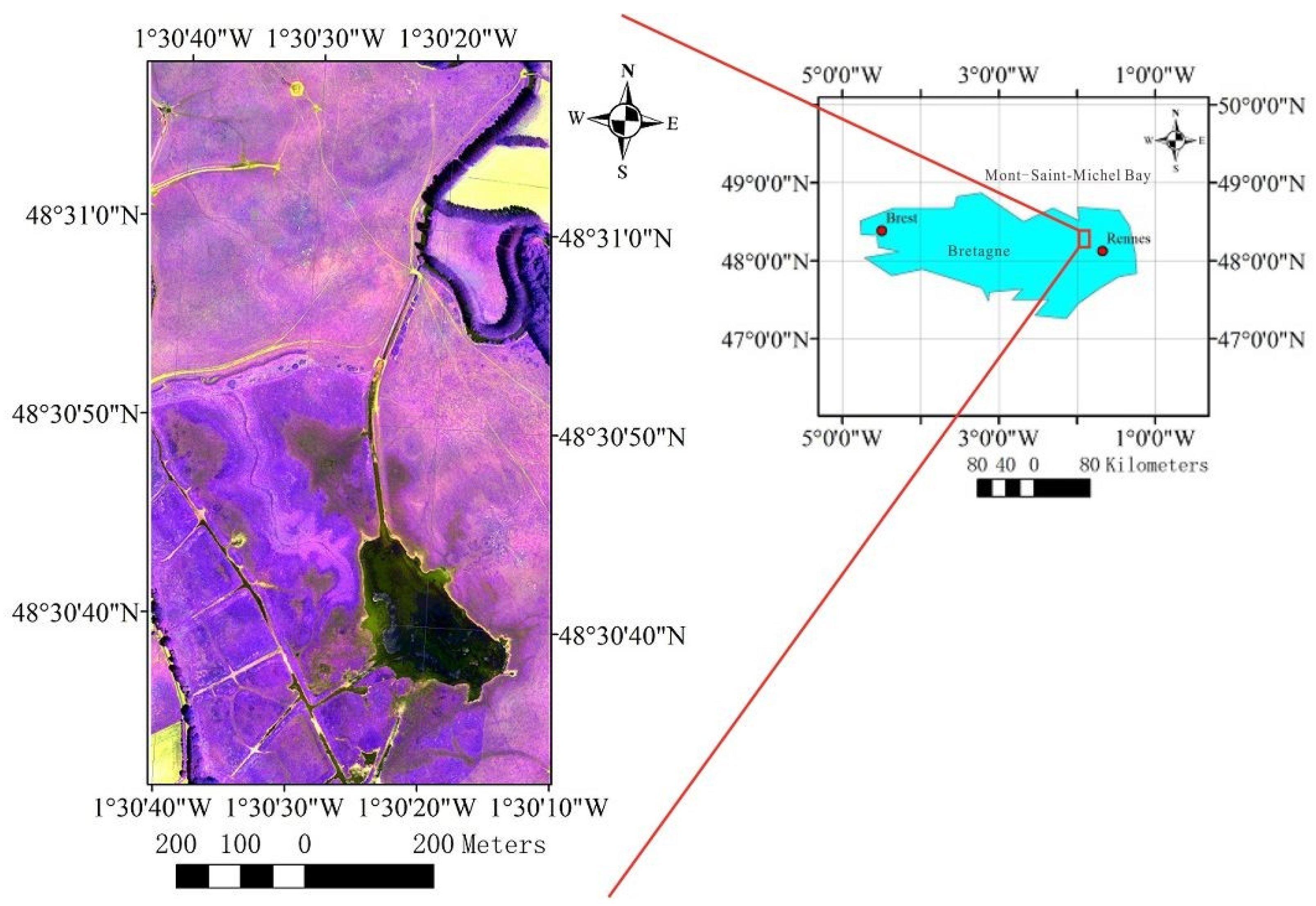
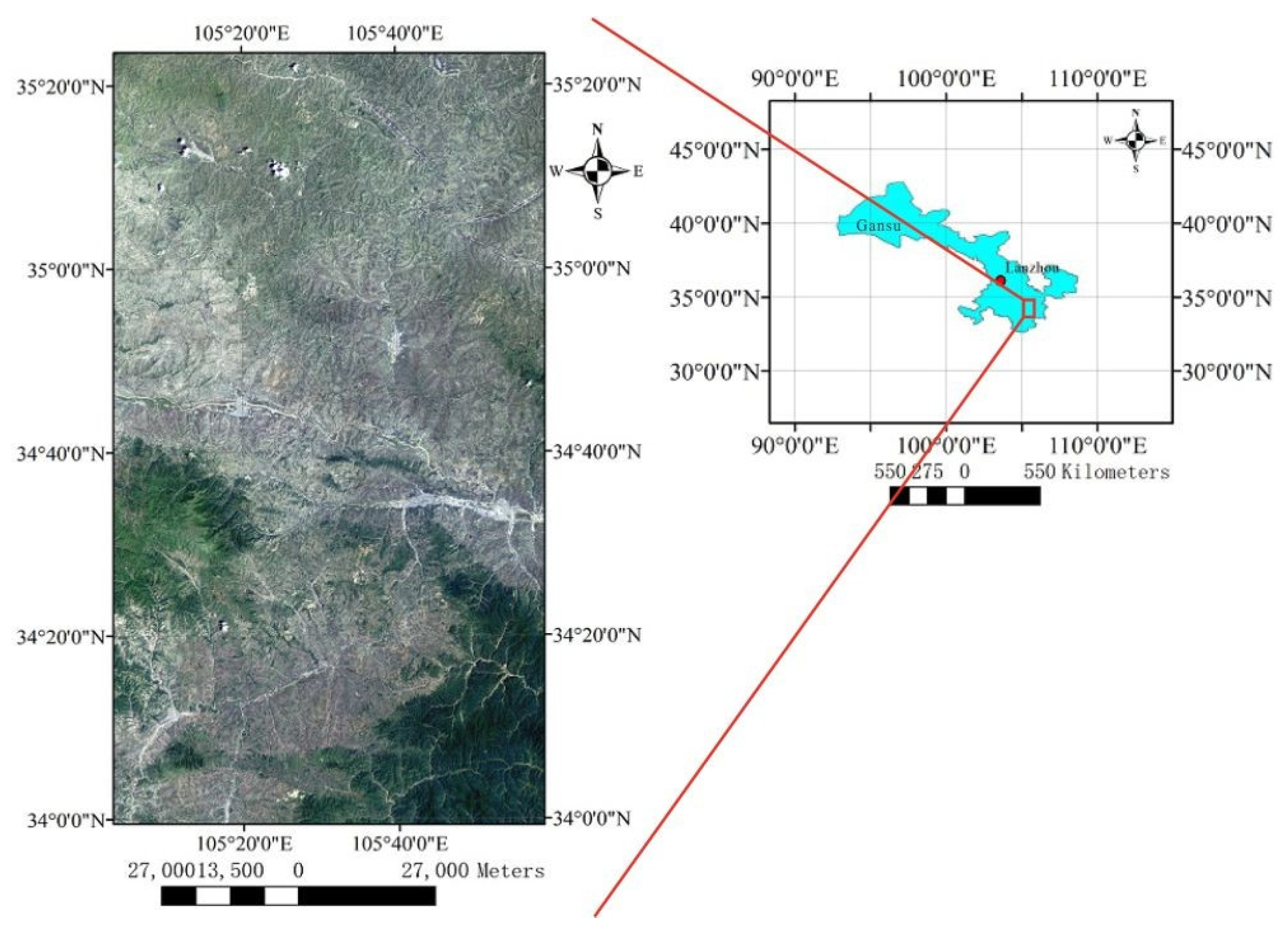
This paper uses unmanned aerial vehicle (UAV) datasets and Landsat-8 datasets for experiments. Figure 1 shows the location of the UAV datasets. Figure 2 shows the location of the Landsat-8 datasets.

UAV datasets are located in Sougéal marsh (western France, 48.52°N, 1.53°W), which is part of the long-term socio-ecological research (LTSER) site Zone Atelier Armorique. This site is a large flooded grassland of 174 hectares located in the floodplain of the Couesnon River, upstream of Mont-Saint-Michel Bay [24]. The projection-type is France Lambert-93. The spatial resolution is 0.02 m. The number of bands is 4: green, red, red-edge, and near-infrared.

Landsat-8 datasets are located in the southeast of Gansu Province (34.73°N, 105.50°E), which is 36 rows and 129 paths in the Worldwide Reference System (WRS-2). The images of these datasets have a small amount of cloud noise in some months. The projection-type is Universal Transverse Mercator (UTM). The spatial resolution is 30 m. The number of bands is 7: coastal, blue, green, red, near-infrared, short-wave infrared-1, and short-wave infrared-2.

2.2. Architecture of Networks

2.2.1. AdaFG Network

Given two images $I_{t_1}$ and $I_{t_2}$ at different times with the same spatial resolution, it is reasonable to assume the image ($I_{estimated}$) at a certain time can be estimated by $I_{t_1}$ and $I_{t_2}$. As is shown in Equation (1):

$$I_{estimated}=b_1\left(x,y\right)\ast K_1\left(x,y\right)+b_2\left(x,y\right)\ast K_2\left(x,y\right)$$

(1)

In Equation (1), $b_1\left(x,y\right)$ and $b_2\left(x,y\right)$ are the patches centered at $\left(x,y\right)$ in $I_{t_1}$ and $I_{t_2}$, and $K_1\left(x,y\right)$ and $K_2\left(x,y\right)$ are a pair of 2D convolution kernels; note that $\ast$ denotes a local convolution operation. The pixel-dependent kernels $K_1$ and $K_2$ capture both motion and re-sampling information required for transformation. The 2D kernels, $K_1$ and $K_2$, could be approximated by a pair of 1D kernels. That is, $K_1$ could be approximated as $k_{1,v}\ast k_{1,h}$ and $K_2$ could be approximated as $k_{2,v}\ast k_{2,h}$. Under this assumption, the main task is to estimate each separable 1D kernel parameter $k_{1,v},k_{1,h},k_{2,v},k_{2,h}$.

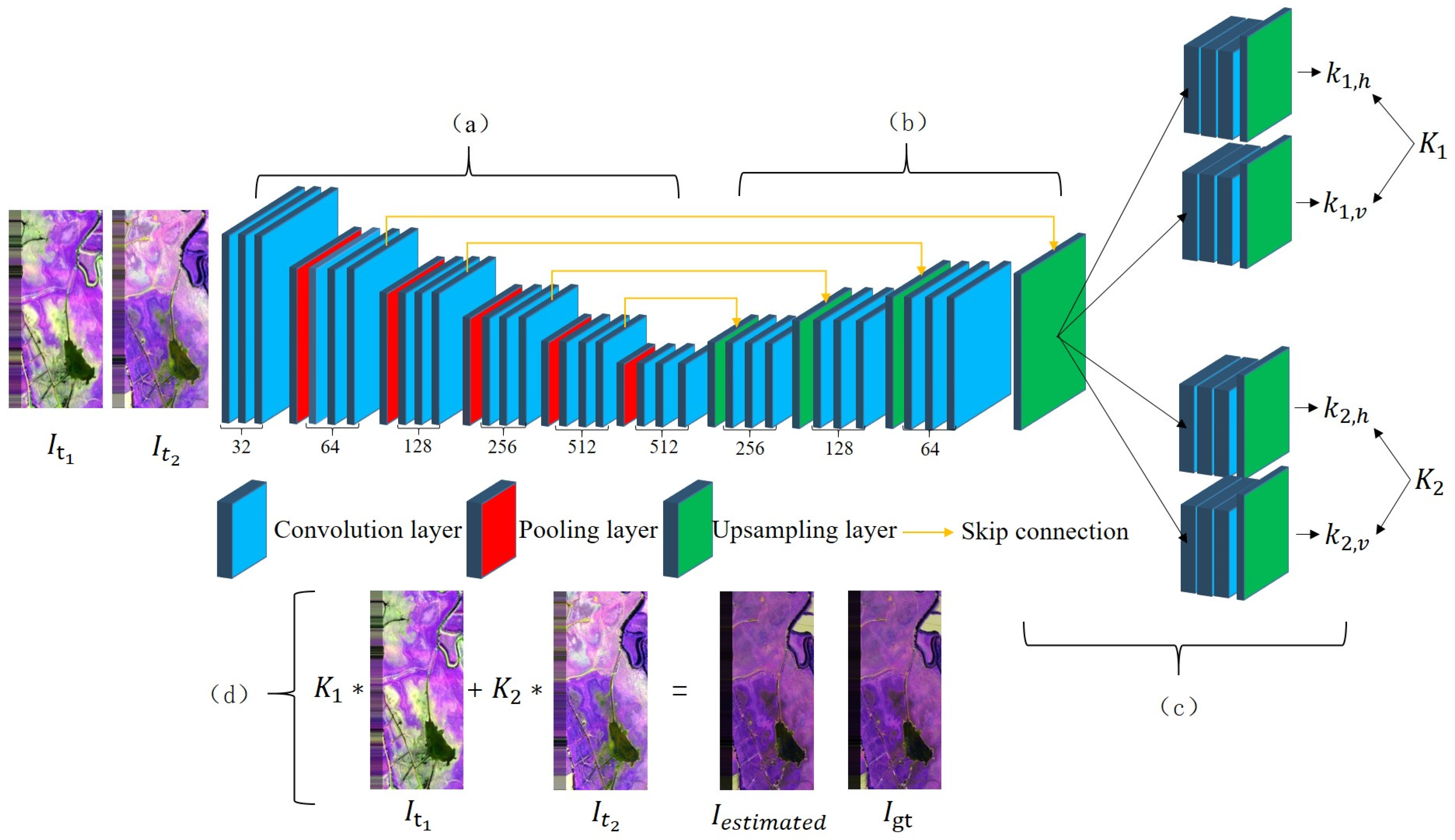
The adaptive filter generation network (AdaFG) consists of a contracting part, an expanding part, a separable convolution part, and a backpropagation part [21]. The architecture of the network is shown in Figure 3.

The extracting part (Figure 3a) is used to extract features of training samples. This part mainly contains five convolution layers (Conv-1, Conv-2, Conv-3, Conv-4 and Conv-5) and pooling layers (Pool-1, Pool-2, Pool-3, Pool-4 and Pool-5). The number of filters in each convolution layer is 32, 64, 128, 256, and 512.

The expanding part (Figure 3b) is used to recover the extracted features. This part mainly contains four deconvolution layers (Deconv-1, Deconv-2, Deconv-3, and Deconv-4) and upsampling layers (Upsample-1, Upsample-2, Upsample-3, and Upsample-4). The number of filters in each deconvolution layer is 512, 256, 128, and 64.

The separable part (Figure 3c) is used to estimate the separable 1D kernel parameter. This part directs the feature information in the last expansion layer into four sub-networks (Subnet-1, Subnet-2, Subnet-3, and Subnet-4), with each sub-network evaluating one 1D kernel.

The backpropagation part (Figure 3d) is used to update the weights of the network in each layer. This part updates the weights of the network in each layer according to the error between the generated result ($I_{estimated}$) and the reference image ($I_{gt}$).

The detailed information of each layer of feature maps in the network is shown in

Table 1. Detailed information of each layer of feature maps in the network.

Type	Kernel Size	Stride	Padding	Feature Maps (Filters × W × H)
Input	—	—	—	2n × 128 × 128
Conv-1	3 × 3	1 × 1	1 × 1	32 × 128 × 128
Pool-1	2 × 2	2 × 2		32 × 64 × 64
Conv-2	3 × 3	1 × 1		64 × 64 × 64
Pool-2	2 × 2	2 × 2		64 × 32 × 32
Conv-3	3 × 3	1 × 1		128 × 32 × 32
Pool-3	2 × 2	2 × 2		128 × 16 × 16
Conv-4	3 × 3	1 × 1		256 × 16 × 16
Pool-4	2 × 2	2 × 2		256 × 8 × 8
Conv-5	3 × 3	1 × 1		512 × 8 × 8
Pool-5	2 × 2	2 × 2		512 × 4 × 4
Deconv-1	3 × 3	1 × 1		512 × 4 × 4
Upsample-1				512 × 8 × 8
Deconv-2				256 × 8 × 8
Upsample-2				256 × 16 × 16
Deconv-3				128 × 16 × 16
Upsample-3				128 × 32 × 32
Deconv-4				64 × 32 × 32
Upsample-4				64 × 64 × 64
Subnet-1				k × 128 × 128
Subnet-2				k × 128 × 128
Subnet-3				k × 128 × 128
Subnet-4				k × 128 × 128

(input image block W × H = 128 × 128, n represents the number of bands, k represents the size of separable convolution kernel).

The size of the feature maps has different calculation equations in different layers of the network. The calculation Equations (2)–(5) inside the convolutional layers, pooling layers, deconvolution layers, and upsampling layers are as follows:

$$W_{conv}=\left(W_{input}-K+2·P\right)/S+1$$

(2)

$$W_{pool}=\left(W_{input}-K\right)/S+1$$

(3)

$$W_{deconv}=\left(W_{input}-1\right)·S+K-2·P$$

(4)

$$W_{upsample}=2·W_{input}$$

(5)

In the above equations, $W_{input}$ represents the input size of samples, $K$, $S$, and $P$ represent the size of kernel, stride, and padding, respectively. $W_{conv}$, $W_{pool}$, $W_{deconv}$, and $W_{upsample}$ represent the output size of feature maps in convolutional layers, pooling layers, deconvolution layers, and upsampling layers, respectively.

Furthermore, the upsampling layers can be executed in various ways, such as nearest-neighbor, bilinear interpolation, and cubic convolution interpolation [25,26,27]. We use skip connection [28,29] to let upsampling layers incorporate features from the contracting part of the AdaFG network.

2.2.2. CLSTM Network

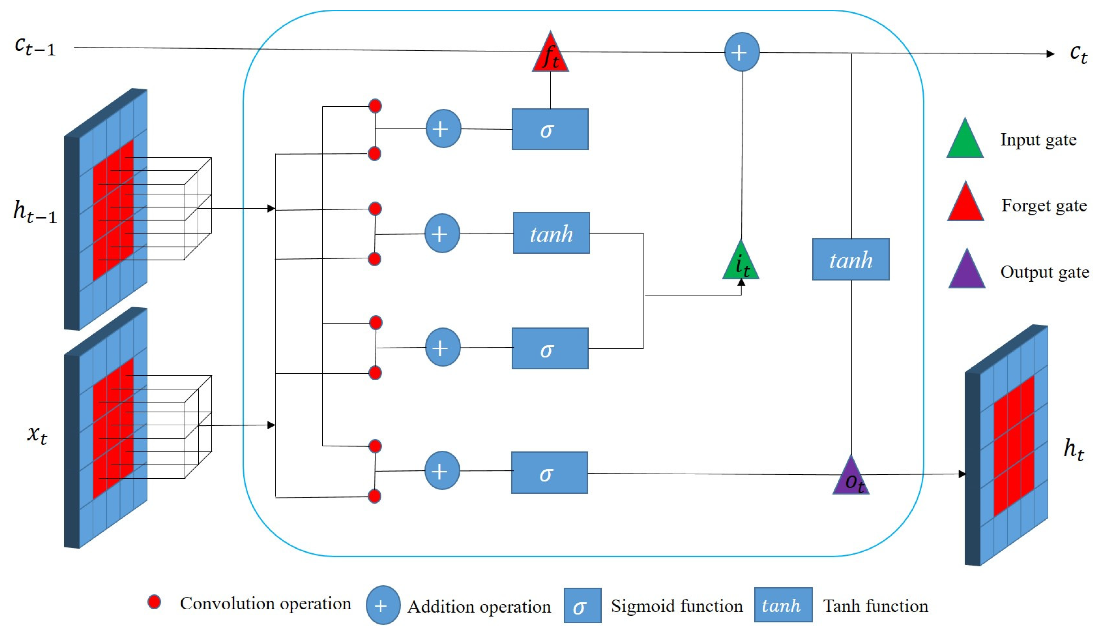
Convolution long short-term memory network (CLSTM) is an improvement based on the long short-term memory network (LSTM) [22]. It mainly focuses on 2D image data and extracts the spatial characteristics of each time point through the convolution operation. Using the principle of LSTM in the time dimension is to learn long-term characteristics, and then conducts long-term series prediction based on the characteristics. This network can grasp the characteristics of space and time. Compared with the LSTM network, the CLSTM network is an end-to-end network model. The transition of input to state and state to state has a convolution structure [30]. The spatial characteristics are extracted through the convolution operation of the image, and then consider the input of new data and the output of the previous time point through the input gate and the forget gate. Finally, the output at this time point is determined through the output gate. The cell structure is shown in Figure 4.

The calculation Equations (6)–(10) inside the CLSTM cell are as follows:

$$f_t=\sigma \left(W_f\ast \left[x_t,h_{t-1}\right]+b_f\right)$$

(6)

$$i_t=\sigma \left(W_i\ast \left[x_t,h_{t-1}\right]+b_i\right)$$

(7)

$$o_t=\sigma \left(W_o\ast \left[x_t,h_{t-1}\right]+b_o\right)$$

(8)

$$c_t=f_t{c}_{t-1}+i_{t}tanh\left(W_c\ast \left[x_t,h_{t-1}\right]+b_c\right)$$

(9)

$$h_t=o_{t}tanh\left(c_t\right)$$

(10)

In the above equations, $\ast$ denotes convolution operation, $x_t$ represents the input of neurons at t, $c_{t-1}$ and $c_t$ represent the cell state of neurons at t−1 and t, $h_{t-1}$ and $h_t$ represent the output of neurons at t−1 and t, $W_f$ and $b_f$ represent the weight and bias of the forget gate ($f_t$),$W_i$ and $b_i$ represent the weight and bias of the input gate ($i_t$), $W_o$ and $b_o$ represent the weight and bias of the output gate ($o_t$), $W_c$ and $b_c$ represent the weight and bias of the cell state, and $\sigma$ represents the sigmoid activation function.

2.2.3. CyGAN Network

Compared with traditional neural networks, the Generative Adversarial Network (GAN) is an unsupervised learning network. GAN has a collapse problem when conducts style conversion between different pictures. Its model is too uncontrollable for larger pictures and more pixels [31,32]. The cycle-consistent generative adversarial network.

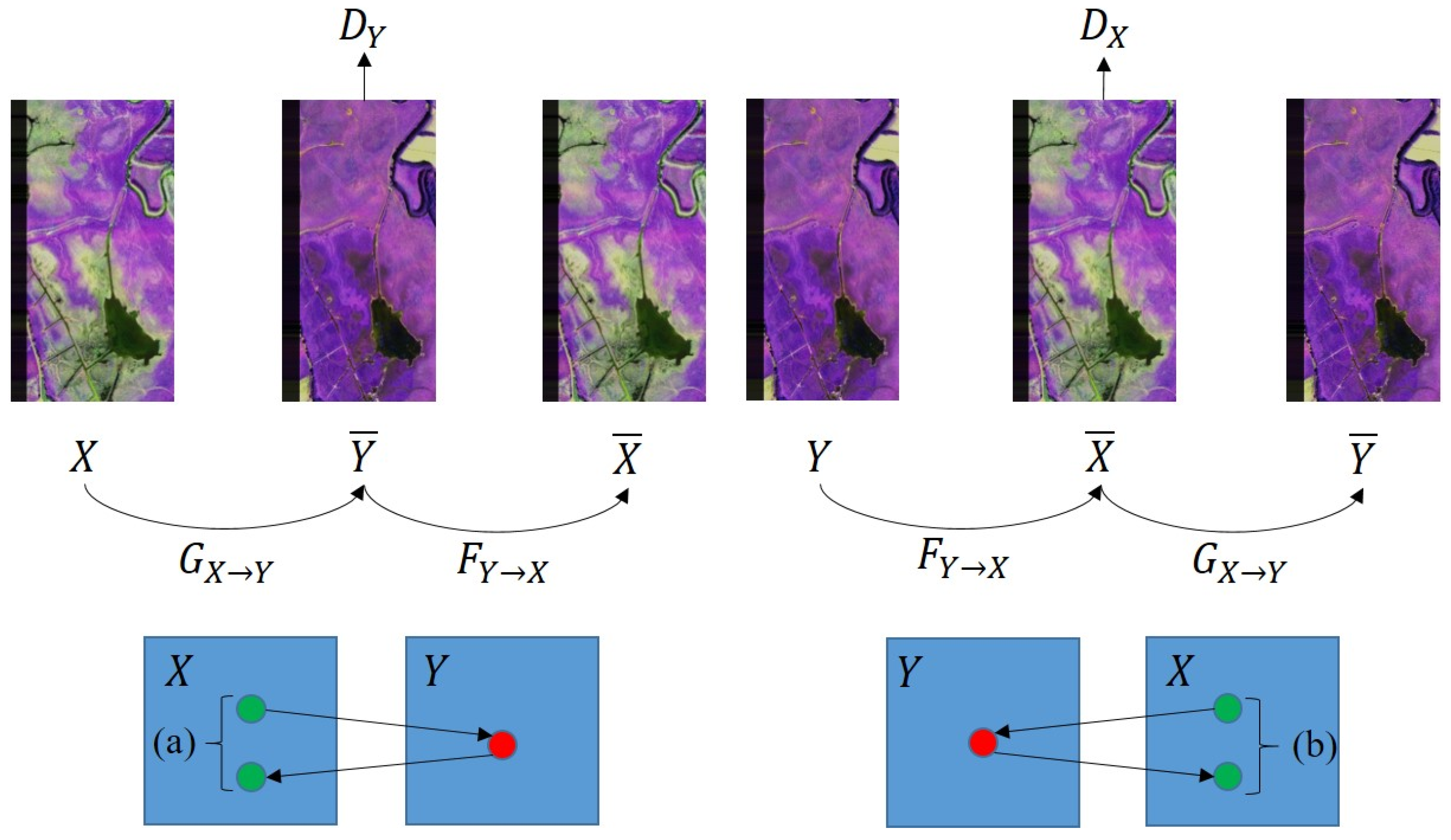
(CyGAN) is an improvement based on the GAN, the purpose of this network is to realize the mutual transformation between a source domain (X) and the target domain (Y) [23]. The structure diagram is shown in Figure 5. CyGAN network mainly contains two mapping functions ($G_{X\to Y}, F_{Y\to X}$) and two corresponding adversarial discriminators ($D_Y$,$D_X$). Meanwhile, there are two cycle-consistent losses: forward and backward cycle-consistent losses.

According to the CyGAN diagram, CyGAN consists of three parts (forward confrontation target, backward confrontation target, and cycle-consistency loss). The calculation Equations (11)–(14) of the forward confrontation target, backward confrontation target, cycle-consistent loss, and objective function are shown as follows:

$$L_{GAN}\left(G,D_Y,X,Y\right)=E_{Y~P_{data}\left(Y\right)}\left[log{D}_Y\left(Y\right)\right]+E_{X~P_{data}\left(X\right)}\left[log\left(1-D_Y\left(G\left(X\right)\right)\right)\right]$$

(11)

$$L_{GAN}\left(F,D_X,Y,X\right)=E_{X~P_{data}\left(X\right)}\left[log{D}_X\left(X\right)\right]+E_{Y~P_{data}\left(Y\right)}\left[log\left(1-D_X\left(F\left(Y\right)\right)\right)\right]$$

(12)

$$L_{cyc}\left(G,F\right)=E_{Y~P_{data}\left(Y\right)}\left[\Vert G\left(F\left(Y\right)\right)-Y{\Vert }_1\right]+E_{X~P_{data}\left(X\right)}\left[\Vert F\left(G\left(X\right)\right)-X{\Vert }_1\right]$$

(13)

$$G*,F*=\arg \underset{G,F}{\underbrace{min}}\underset{D_Y,D_X}{\underbrace{max}}\left\{{\mu }_1{L}_{cyc}\left(G,F\right)+{\mu }_2\left(L_{GAN}\left(G,D_Y,X,Y\right)+L_{GAN}\left(F,D_X,Y,X\right)\right)\right\}$$

(14)

In the above equations, X and Y represent the real image in the source domain and target domain, G(X) and F(Y) represent generated images, $P_{data}\left(X\right)$ and $P_{data}\left(Y\right)$ represent the distribution of real image in the target domain, ~ represents the obey relationship, E represents the mathematical expectation function, ${\mu }_1$ and ${\mu }_2$ represent proportional hyper-parameter of the cycle-consistent loss and the confrontation target.

2.3. Evaluation Indicator

Our research uses root mean square error (RMSE) and entropy function to evaluate the quality of the generated result: RMSE measures the pixel error between a generated image $I_{estimated}$ and corresponding reference image $I_{gt}$, as defined in Equation (15):

$$RMSE=\sqrt{\frac{1}{\mathrm{W}\times \mathrm{H}}\mathsf{\Sigma }\left({\left|\left|I_{estimated}-I_{gt}\right|\right|}_2\right)}$$

(15)

The entropy function based on statistical features is an important indicator to measure the richness of image information. The information amount of a generated image $I_{estimated}$ is measured by the information entropy D($I_{estimated}$), as defined in Equation (16):

$$D\left(I_{estimated}\right)=-{\displaystyle \sum }_{i=0}^L{P}_{i}ln\left(P_i\right)$$

(16)

In Equation (16), P_i is the probability of a pixel with a gray value of i in image, and L is the total number of gray levels (L = 255). According to Shannon’s information theory [33], there is the most information when there is maximum entropy.

3. Results and Analysis

3.1. Experimental Strategy

The size of scenes in sequence in both datasets was 3072 × 5632. To get enough training samples, all scenes in a sequence were cropped as a block with a size of 128 × 128.

This paper mainly conducted three aspects. The first aspect was a generalized application in the time dimension using different deep convolution networks. The second and third aspects were mainly to construct datasets in different time series using single and multiple networks, and this was implemented among multiple sequences. Corresponding experimental data are described in the following paragraphs in detail.

Before describing the experimental data in every aspect, we will first introduce some symbols used below. We represent image scene in different sequences, and $I_{t_i}$, $I_{t_i}^{\prime }$, $I_{t_i}^{″}$ represent different sequence images acquired at time $t_i$ ($t_i$ = 1,…,12). In AdaFG network, the mapping model is expressed as $f_{\left[I_{t_1}, I_{t_2},I_{t_3}\right]}$, where [$I_{t_1}, I_{t_2}, I_{t_3}$] represents training image triples, $I_{t_1}$ and $I_{t_2}$ represent the training image pairs, $I_{t_3}$ represents the reference image, t₁ and t₂ represent the month of training image pairs acquired, and t₃ represents the month of the reference image acquired. $f_{\left[I_{t_1}, I_{t_2},I_{t_3}\right]}\left(I_{t_1}^{\prime },I_{t_2}^{\prime }\right)$ represents output image with mapping model $f_{\left[I_{t_1}, I_{t_2},I_{t_3}\right]}$ and input scenes $I_{t_1}^{\prime }$ and $I_{t_2}^{\prime }$. In CLSTM network, the mapping model is expressed as $f_{\left[I_{t_1},\dots , I_{t_n},I_{t_{n+1}}\right]}$, where [$I_{t_1},\dots , I_{t_n}, I_{t_{n+1}}$] represents training image multi-group, $I_{t_1},\dots , I_{t_n}$ represent the training images, $I_{t_{n+1}}$ represents the reference image, t₁,…,t_n represent the month of training images acquired, and t_n+1 represents the month of the reference image acquired. $f_{\left[I_{t_1},\dots , I_{t_n},I_{t_{n+1}}\right]}\left(I_{t_1}^{\prime },\dots ,I_{t_n}^{\prime }\right)$ represents output image with mapping model $f_{\left[I_{t_1},\dots , I_{t_n},I_{t_{n+1}}\right]}$ and input scenes $I_{t_1}^{\prime },\dots ,I_{t_n}^{\prime }$. In CyGAN network, the output image is expressed as $f_{\left[I_{t_1}, I_{t_2}\right]}\left(I_{t_1}^{\prime }\right)$, where $f_{\left[I_{t_1}, I_{t_2}\right]}$ represents a mapping model trained by training image pair [$I_{t_1}, I_{t_2}$] with reference image $I_{t_2}$. $I_{t_1}^{\prime }$ in the brackets represents the input used to generate the output image.

Table 2. Name and date of experimental datasets in the first aspect.

Datasets	Image Names	Image Dates
UAV	$I_4$	April 2019
	$I_5$	May 2019
	$I_6$	June 2019
	$I_7$	July 2019
	$I_8$	August 2019
Landsat-8	$I_4^{\prime }$	April 2014
	$I_7^{\prime }$	July 2014
	$I_2^{\prime }$	February 2014
	$I_8^{\prime }$	August 2014
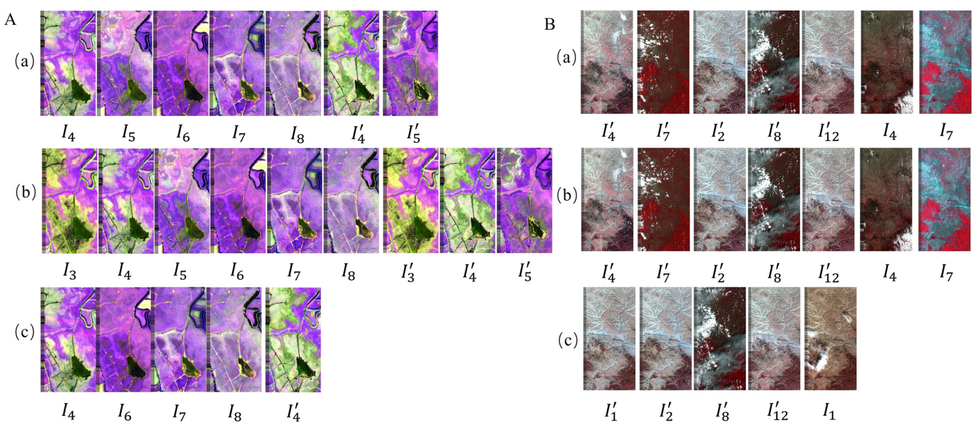
	$I_{12}^{\prime }$	December 2014

shows the sequences used in the first aspect and the dates of all scenes acquired in them. Figure 6 shows the visual effect of training and testing images using different deep convolution networks in the first aspect.

The second and third aspects mainly constructed remote-sensing sequence datasets with multiple sequences. The remote-sensing sequence here mainly reflected two aspects: non-equidistant missing images in the same sequence and non-equidistant missing images of the same scene in a different sequence. It was difficult to find an analysis method to analyze these sequences in a unified and integrated manner. The number of images in a year was relatively small, and the time interval between images was uncertain.

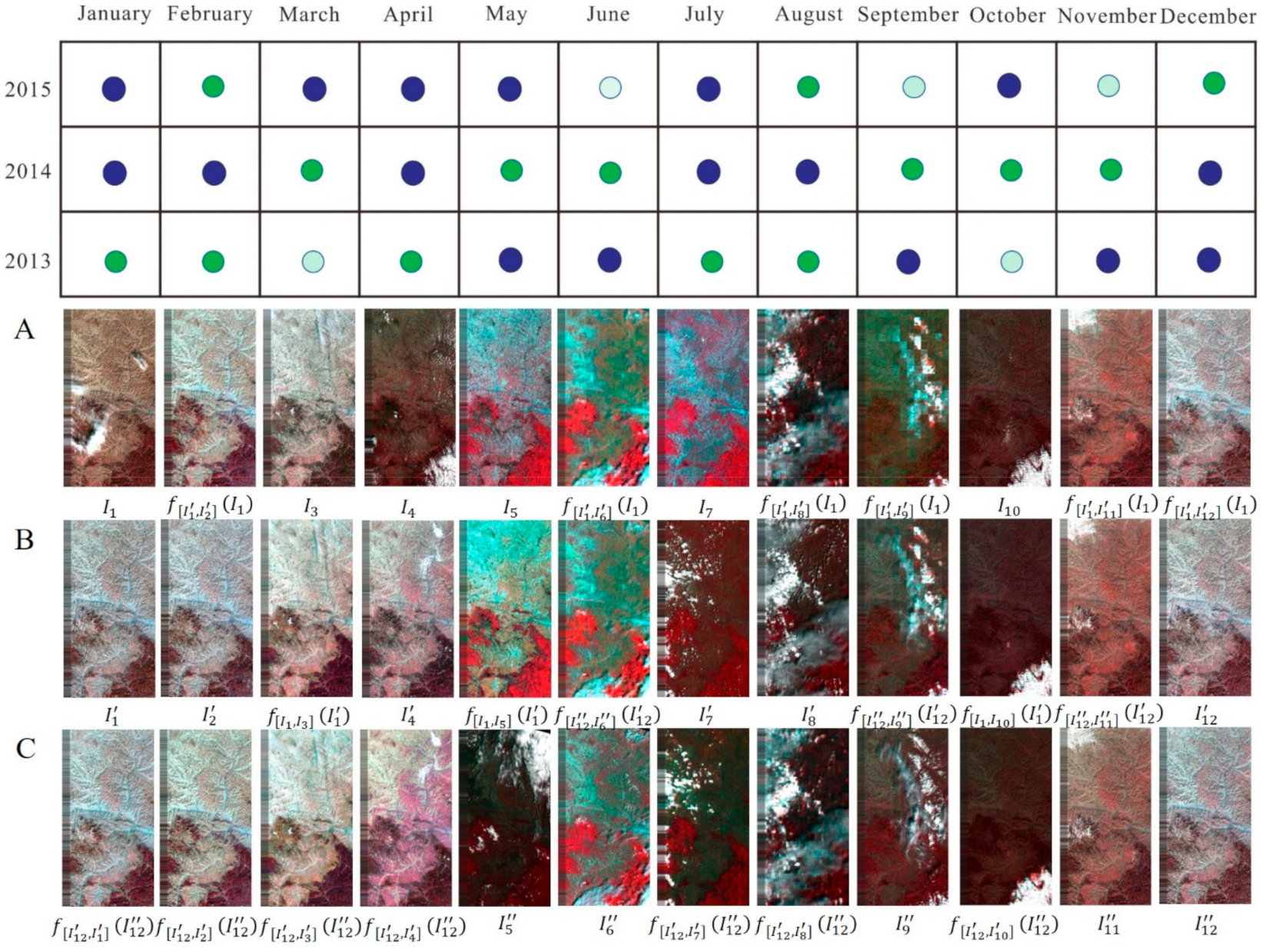
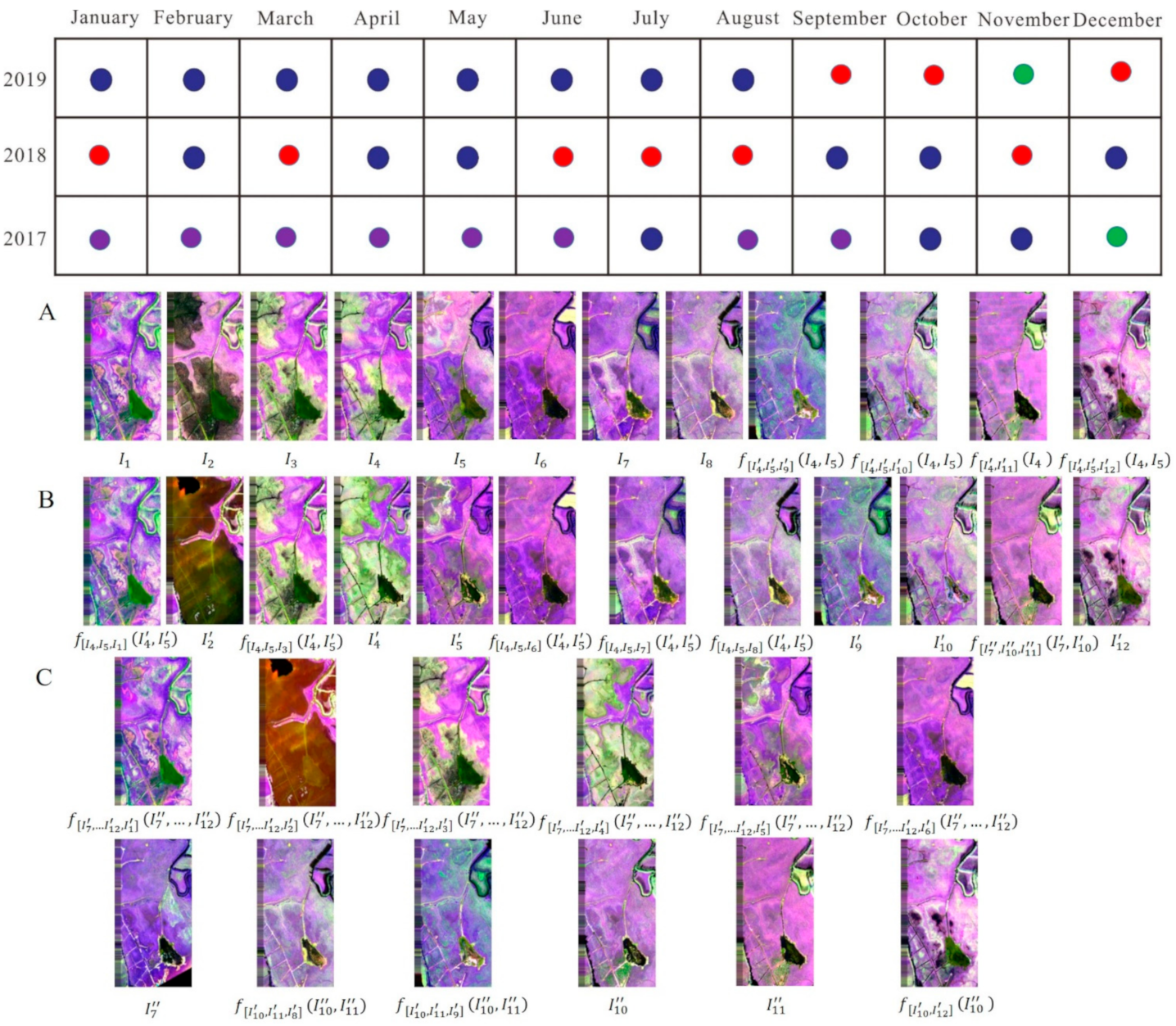
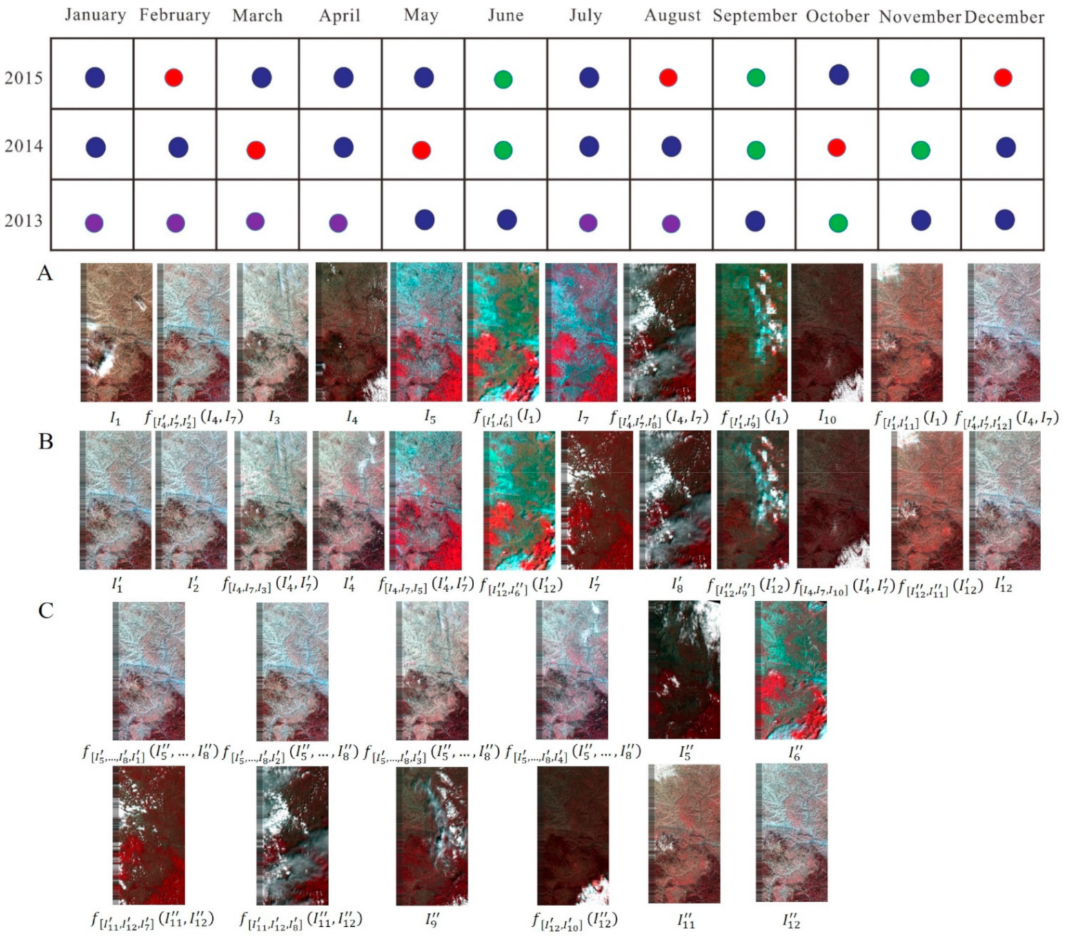
Figure 7A shows available UAV images from 2017 to 2019 and Landsat-8 images from 2013 to 2015 in the second and third aspects. It is obvious that there are many missing images for the frequency of one image per month. Figure 7B shows one construction strategy with a single network. In UAV datasets, the crimson, red, and light-red points mark the first, second, and third-level generated result, in which training and testing images are listed in

Table 3. Training, testing, and output images with AdaFG in UAV datasets.

Color.	Training Images	Testing Images	Output Images
Crimson	$I_4,I_5,I_1$	$I_4^{\prime },I_5^{\prime }$	$f_{\left[I_4,I_5,I_1\right]}\left(I_4^{\prime },I_5^{\prime }\right)$
	$I_4,I_5,I_3$		$f_{\left[I_4,I_5,I_3\right]}\left(I_4^{\prime },I_5^{\prime }\right)$
	$I_4,I_5,I_6$		$f_{\left[I_4,I_5,I_6\right]}\left(I_4^{\prime },I_5^{\prime }\right)$
	$I_4,I_5,I_7$		$f_{\left[I_4,I_5,I_7\right]}\left(I_4^{\prime },I_5^{\prime }\right)$
	$I_4,I_5,I_8$		$f_{\left[I_4,I_5,I_8\right]}\left(I_4^{\prime },I_5^{\prime }\right)$
	$I_4^{\prime },I_5^{\prime },I_9^{\prime }$	$I_4,I_5$	$f_{\left[I_4^{\prime },I_5^{\prime },I_9^{\prime }\right]}\left(I_4,I_5\right)$
	$I_4^{\prime },I_5^{\prime },I_{10}^{\prime }$		$f_{\left[I_4^{\prime },I_5^{\prime },I_{10}^{\prime }\right]}\left(I_4,I_5\right)$
	$I_4^{\prime },I_5^{\prime },I_{12}^{\prime }$		$f_{\left[I_4^{\prime },I_5^{\prime },I_{12}^{\prime }\right]}\left(I_4,I_5\right)$
Red	$I_7^{″},I_{10}^{″},I_{11}^{″}$	$I_7^{\prime },I_{10}^{\prime }$	$f_{\left[I_7^{″},I_{10}^{″},I_{11}^{″}\right]}\left(I_7^{\prime },I_{10}^{\prime }\right)$
Light-red	$I_4^{\prime },I_5^{\prime },I_{11}^{\prime }$	$I_4,I_5$	$f_{\left[I_4^{\prime },I_5^{\prime },I_{11}^{\prime }\right]}\left(I_4,I_5\right)$
	$I_{10}^{\prime },I_{11}^{\prime },I_1^{\prime }$	$I_{10}^{″},I_{11}^{″}$	$f_{\left[I_{10}^{\prime },I_{11}^{\prime },I_1^{\prime }\right]}\left(I_{10}^{″},I_{11}^{″}\right)$
	$I_{10}^{\prime },I_{11}^{\prime },I_2^{\prime }$		$f_{\left[I_{10}^{\prime },I_{11}^{\prime },I_2^{\prime }\right]}\left(I_{10}^{″},I_{11}^{″}\right)$
	$I_{10}^{\prime },I_{11}^{\prime },I_3^{\prime }$		$f_{\left[I_{10}^{\prime },I_{11}^{\prime },I_3^{\prime }\right]}\left(I_{10}^{″},I_{11}^{″}\right)$
	$I_{10}^{\prime },I_{11}^{\prime },I_4^{\prime }$		$f_{\left[I_{10}^{\prime },I_{11}^{\prime },I_4^{\prime }\right]}\left(I_{10}^{″},I_{11}^{″}\right)$
	$I_{10}^{\prime },I_{11}^{\prime },I_5^{\prime }$		$f_{\left[I_{10}^{\prime },I_{11}^{\prime },I_5^{\prime }\right]}\left(I_{10}^{″},I_{11}^{″}\right)$
	$I_{10}^{\prime },I_{11}^{\prime },I_6^{\prime }$		$f_{\left[I_{10}^{\prime },I_{11}^{\prime },I_6^{\prime }\right]}\left(I_{10}^{″},I_{11}^{″}\right)$
	$I_{10}^{\prime },I_{11}^{\prime },I_8^{\prime }$		$f_{\left[I_{10}^{\prime },I_{11}^{\prime },I_8^{\prime }\right]}\left(I_{10}^{″},I_{11}^{″}\right)$
	$I_{10}^{\prime },I_{11}^{\prime },I_9^{\prime }$		$f_{\left[I_{10}^{\prime },I_{11}^{\prime },I_9^{\prime }\right]}\left(I_{10}^{″},I_{11}^{″}\right)$
	$I_{10}^{\prime },I_{11}^{\prime },I_{12}^{\prime }$		$f_{\left[I_{10}^{\prime },I_{11}^{\prime },I_{12}^{\prime }\right]}\left(I_{10}^{″},I_{11}^{″}\right)$

. In Landsat-8 datasets, the dark-green and light-green points mark the first and second generated result, in which training and testing images are listed in

Table 4. Training, testing, and output images with CyGAN in Landsat-8 datasets.

Color	Training Images	Testing Images	Output Images
Dark-green	$I_1^{\prime },I_2^{\prime }$	$I_1$	$f_{\left[I_1^{\prime },I_2^{\prime }\right]}\left(I_1\right)$
	$I_1^{\prime },I_8^{\prime }$		$f_{\left[I_1^{\prime },I_8^{\prime }\right]}\left(I_1\right)$
	$I_1^{\prime },I_{12}^{\prime }$		$f_{\left[I_1^{\prime },I_{12}^{\prime }\right]}\left(I_1\right)$
	$I_1,I_3$	$I_1^{\prime }$	$f_{\left[I_1,I_3\right]}\left(I_1^{\prime }\right)$
	$I_1,I_5$		$f_{\left[I_1,I_5\right]}\left(I_1^{\prime }\right)$
	$I_1,I_{10}$		$f_{\left[I_1,I_{10}\right]}\left(I_1^{\prime }\right)$
	$I_{12}^{″},I_6^{″}$	$I_{12}^{\prime }$	$f_{\left[I_{12}^{″},I_6^{″}\right]}\left(I_{12}^{\prime }\right)$
	$I_{12}^{″},I_9^{″}$		$f_{\left[I_{12}^{″},I_9^{″}\right]}\left(I_{12}^{\prime }\right)$
	$I_{12}^{″},I_{11}^{″}$		$f_{\left[I_{12}^{″},I_{11}^{″}\right]}\left(I_{12}^{\prime }\right)$
	$I_{12}^{\prime },I_1^{\prime }$	$I_{12}^{″}$	$f_{\left[I_{12}^{\prime },I_1^{\prime }\right]}\left(I_{12}^{″}\right)$
	$I_{12}^{\prime },I_2^{\prime }$		$f_{\left[I_{12}^{\prime },I_2^{\prime }\right]}\left(I_{12}^{″}\right)$
	$I_{12}^{\prime },I_4^{\prime }$		$f_{\left[I_{12}^{\prime },I_4^{\prime }\right]}\left(I_{12}^{″}\right)$
	$I_{12}^{\prime },I_7^{\prime }$		$f_{\left[I_{12}^{\prime },I_7^{\prime }\right]}\left(I_{12}^{″}\right)$
	$I_{12}^{\prime },I_8^{\prime }$		$f_{\left[I_{12}^{\prime },I_8^{\prime }\right]}\left(I_{12}^{″}\right)$
Light-green	$I_1^{\prime },I_6^{\prime }$	$I_1$	$f_{\left[I_1^{\prime },I_6^{\prime }\right]}\left(I_1\right)$
	$I_1^{\prime },I_9^{\prime }$		$f_{\left[I_1^{\prime },I_9^{\prime }\right]}\left(I_1\right)$
	$I_1^{\prime },I_{11}^{\prime }$		$f_{\left[I_1^{\prime },I_{11}^{\prime }\right]}\left(I_1\right)$
	$I_{12}^{\prime },I_3^{\prime }$	$I_{12}^{″}$	$f_{\left[I_{12}^{\prime },I_3^{\prime }\right]}\left(I_{12}^{″}\right)$
	$I_{12}^{\prime },I_{10}^{\prime }$		$f_{\left[I_{12}^{\prime },I_{10}^{\prime }\right]}\left(I_{12}^{″}\right)$

. Figure 7C shows one construction strategy with multiple networks. The red, green, and purple points mark the generated result with AdaFG, CyGAN, and CLSTM network in both datasets, in which training and testing images are listed in

Table 5. Training, testing, and output images with AdaFG, CyGAN, and CLSTM in UAV datasets.

Networks.	Training Images	Testing Images	Output Images
AdaFG	$I_4,I_5,I_1$	$I_4^{\prime },I_5^{\prime }$	$f_{\left[I_4,I_5,I_1\right]}\left(I_4^{\prime },I_5^{\prime }\right)$
	$I_4,I_5,I_3$		$f_{\left[I_4,I_5,I_3\right]}\left(I_4^{\prime },I_5^{\prime }\right)$
	$I_4,I_5,I_6$		$f_{\left[I_4,I_5,I_6\right]}\left(I_4^{\prime },I_5^{\prime }\right)$
	$I_4,I_5,I_7$		$f_{\left[I_4,I_5,I_7\right]}\left(I_4^{\prime },I_5^{\prime }\right)$
	$I_4,I_5,I_8$		$f_{\left[I_4,I_5,I_8\right]}\left(I_4^{\prime },I_5^{\prime }\right)$
	$I_4^{\prime },I_5^{\prime },I_9^{\prime }$	$I_4,I_5$	$f_{\left[I_4^{\prime },I_5^{\prime },I_9^{\prime }\right]}\left(I_4,I_5\right)$
	$I_4^{\prime },I_5^{\prime },I_{10}^{\prime }$		$f_{\left[I_4^{\prime },I_5^{\prime },I_{10}^{\prime }\right]}\left(I_4,I_5\right)$
	$I_4^{\prime },I_5^{\prime },I_{12}^{\prime }$		$f_{\left[I_4^{\prime },I_5^{\prime },I_{12}^{\prime }\right]}\left(I_4,I_5\right)$
	$I_7^{″},I_{10}^{″},I_{11}^{″}$	$I_7^{\prime },I_{10}^{\prime }$	$f_{\left[I_7^{″},I_{10}^{″},I_{11}^{″}\right]}\left(I_7^{\prime },I_{10}^{\prime }\right)$
CyGAN	$I_4^{\prime },I_{11}^{\prime }$	$I_4$	$f_{\left[I_4^{\prime },I_{11}^{\prime }\right]}\left(I_4\right)$
	$I_{10}^{\prime },I_{12}^{\prime }$	$I_{10}^{″}$	$f_{\left[I_{10}^{\prime },I_{12}^{\prime }\right]}\left(I_{10}^{″}\right)$
CLSTM	$I_{10}^{\prime },I_{11}^{\prime },I_8^{\prime },I_9^{\prime }$	$I_{10}^{″},I_{11}^{″}$	$f_{\left[I_{10}^{\prime },I_{11}^{\prime },I_8^{\prime }\right]}\left(I_{10}^{″},I_{11}^{″}\right)$
			$f_{\left[I_{10}^{\prime },I_{11}^{\prime },I_9^{\prime }\right]}\left(I_{10}^{″},I_{11}^{″}\right)$
	$I_7^{\prime },I_8^{\prime },I_9^{\prime },I_{10}^{\prime },I_{11}^{\prime },I_{12}^{\prime }$  $I_1^{\prime },I_2^{\prime },I_3^{\prime },I_4^{\prime },I_5^{\prime },I_6^{\prime }$	$I_7^{″},I_8^{″},I_9^{″},I_{10}^{″},I_{11}^{″},I_{12}^{″}$	$f_{\left[I_7^{\prime },\dots ,I_{12}^{\prime },I_1^{\prime }\right]}\left(I_7^{″},\dots ,I_{12}^{″}\right)$
			$f_{\left[I_7^{\prime },\dots ,I_{12}^{\prime },I_2^{\prime }\right]}\left(I_7^{″},\dots ,I_{12}^{″}\right)$
			$f_{\left[I_7^{\prime },\dots ,I_{12}^{\prime },I_3^{\prime }\right]}\left(I_7^{″},\dots ,I_{12}^{″}\right)$
			$f_{\left[I_7^{\prime },\dots ,I_{12}^{\prime },I_4^{\prime }\right]}\left(I_7^{″},\dots ,I_{12}^{″}\right)$
			$f_{\left[I_7^{\prime },\dots ,I_{12}^{\prime },I_5^{\prime }\right]}\left(I_7^{″},\dots ,I_{12}^{″}\right)$
			$f_{\left[I_7^{\prime },\dots ,I_{12}^{\prime },I_6^{\prime }\right]}\left(I_7^{″},\dots ,I_{12}^{″}\right)$

and

Table 6. Training, testing, and output images with AdaFG, CyGAN, and CLSTM in Landsat-8 datasets.

Networks	Training Images	Testing Images	Output Images
AdaFG	$I_4^{\prime },I_7^{\prime },I_2^{\prime }$	$I_4,I_7$	$f_{\left[I_4^{\prime },I_7^{\prime },I_2^{\prime }\right]}\left(I_4,I_7\right)$
	$I_4^{\prime },I_7^{\prime },I_8^{\prime }$		$f_{\left[I_4^{\prime },I_7^{\prime },I_8^{\prime }\right]}\left(I_4,I_7\right)$
	$I_4^{\prime },I_7^{\prime },I_{12}^{\prime }$		$f_{\left[I_4^{\prime },I_7^{\prime },I_{12}^{\prime }\right]}\left(I_4,I_7\right)$
	$I_4,I_7,I_3$	$I_4^{\prime },I_7^{\prime }$	$f_{\left[I_4,I_7,I_3\right]}\left(I_4^{\prime },I_7^{\prime }\right)$
	$I_4,I_7,I_5$		$f_{\left[I_4,I_7,I_5\right]}\left(I_4^{\prime },I_7^{\prime }\right)$
	$I_4,I_7,I_{10}$		$f_{\left[I_4,I_7,I_{10}\right]}\left(I_4^{\prime },I_7^{\prime }\right)$
CyGAN	$I_{12}^{″},I_6^{″}$	$I_{12}^{\prime }$	$f_{\left[I_{12}^{″},I_6^{″}\right]}\left(I_{12}^{\prime }\right)$
	$I_{12}^{″},I_9^{″}$		$f_{\left[I_{12}^{″},I_9^{″}\right]}\left(I_{12}^{\prime }\right)$
	$I_{12}^{″},I_{11}^{″}$		$f_{\left[I_{12}^{″},I_{11}^{″}\right]}\left(I_{12}^{\prime }\right)$
	$I_1^{\prime },I_6^{\prime }$	$I_1$	$f_{\left[I_1^{\prime },I_6^{\prime }\right]}\left(I_1\right)$
	$I_1^{\prime },I_9^{\prime }$		$f_{\left[I_1^{\prime },I_9^{\prime }\right]}\left(I_1\right)$
	$I_1^{\prime },I_{11}^{\prime }$		$f_{\left[I_1^{\prime },I_{11}^{\prime }\right]}\left(I_1\right)$
	$I_{12}^{\prime },I_{10}^{\prime }$	$I_{12}^{″}$	$f_{\left[I_{12}^{\prime },I_{10}^{\prime }\right]}\left(I_{12}^{″}\right)$
CLSTM	$I_{11}^{\prime },I_{12}^{\prime },I_7^{\prime },I_8^{\prime }$	$I_{11}^{″},I_{12}^{″}$	$f_{\left[I_{11}^{\prime },I_{12}^{\prime },I_7^{\prime }\right]}\left(I_{11}^{″},I_{12}^{″}\right)$
			$f_{\left[I_{11}^{\prime },I_{12}^{\prime },I_8^{\prime }\right]}\left(I_{11}^{″},I_{12}^{″}\right)$
	$I_5^{\prime },I_6^{\prime },I_7^{\prime },I_8^{\prime }$ $I_1^{\prime },I_2^{\prime },I_3^{\prime },I_4^{\prime }$	$I_5^{″},I_6^{″},I_7^{″},I_8^{″}$	$f_{\left[I_5^{\prime },\dots ,I_8^{\prime },I_1^{\prime }\right]}\left(I_5^{″},\dots ,I_8^{″}\right)$
			$f_{\left[I_5^{\prime },\dots ,I_8^{\prime },I_2^{\prime }\right]}\left(I_5^{″},\dots ,I_8^{″}\right)$
			$f_{\left[I_5^{\prime },\dots ,I_8^{\prime },I_3^{\prime }\right]}\left(I_5^{″},\dots ,I_8^{″}\right)$
			$f_{\left[I_5^{\prime },\dots ,I_8^{\prime },I_4^{\prime }\right]}\left(I_5^{″},\dots ,I_8^{″}\right)$

.

3.2. Experimental Details

Hyper-parameters selection: We used a separate convolution kernel of size 11 in the AdaFG network, used stacks of 3 × 3 CLSTM network layer, and set ${\mu }_1=$350, ${\mu }_2=$1/32 in CyGAN network. Meanwhile, we used the mean square error (MSE) as the loss function. The optimizer used in the training was Adamax with ${\beta }_1$= 0.9, ${\beta }_2$= 0.99, and a learning rate of 0.001. Compared to other network optimizers, Adamax could achieve better convergence of the model [34].

Time Complexity: We used the python machine learning library to execute the deep convolution networks. To improve computational efficiency, we organized our layer in computer unified device architecture (CUDA). Our deep convolution networks were able to generate a 256 × 256 image block in 4 s. Obtaining the overall scene image (image size 3072 × 5632) took about 18 min under the acceleration of the graphics processing unit (GPU) [35].

3.3. Experimental Results

3.3.1. Generalization of Networks

Table 7. Quantitative evaluation between the generated result and the reference image.

Datasets	Generated Results	Reference Images	Entropy	RMSE (Pixel)
UAV	$f_{\left[I_4,I_5,I_6\right]}\left(I_4^{\prime },I_5^{\prime }\right)$	I6	3.658	1.128
	$f_{\left[I_3,I_4,I_5,I_6\right]}\left(I_3^{\prime },I_4^{\prime },I_5^{\prime }\right)$		3.625	1.758
	$f_{\left[I_4,I_6\right]}\left(I_4^{\prime }\right)$		3.592	3.585
	$f_{\left[I_4,I_5,I_7\right]}\left(I_4^{\prime },I_5^{\prime }\right)$	I7	3.355	0.952
	$f_{\left[I_3,I_4,I_5,I_7\right]}\left(I_3^{\prime },I_4^{\prime },I_5^{\prime }\right)$		3.330	1.300
	$f_{\left[I_4,I_7\right]}\left(I_4^{\prime }\right)$		3.305	3.077
	$f_{\left[I_4,I_5,I_8\right]}\left(I_4^{\prime },I_5^{\prime }\right)$	I8	3.482	0.954
	$f_{\left[I_3,I_4,I_5,I_8\right]}\left(I_3^{\prime },I_4^{\prime },I_5^{\prime }\right)$		3.455	1.421
	$f_{\left[I_4,I_8\right]}\left(I_4^{\prime }\right)$		3.426	3.690
Landsat-8	$f_{\left[I_4^{\prime },I_7^{\prime },I_2^{\prime }\right]}\left(I_4,I_7\right)$	$I_2^{\prime }$	3.064	1.144
	$f_{\left[I_4^{\prime },I_7^{\prime },I_2^{\prime }\right]}\left(I_4,I_7\right)$		2.975	1.537
	$f_{\left[I_1^{\prime },I_2^{\prime }\right]}\left(I_1\right)$		2.905	2.694
	$f_{\left[I_4^{\prime },I_7^{\prime },I_8^{\prime }\right]}\left(I_4,I_7\right)$	$I_8^{\prime }$	3.830	1.170
	$f_{\left[I_4^{\prime },I_7^{\prime },I_8^{\prime }\right]}\left(I_4,I_7\right)$		3.830	1.681
	$f_{\left[I_1^{\prime },I_8^{\prime }\right]}\left(I_1\right)$		3.777	5.017
	$f_{\left[I_4^{\prime },I_7^{\prime },I_{12}^{\prime }\right]}\left(I_4,I_7\right)$	$I_{12}^{\prime }$	2.994	0.929
	$f_{\left[I_4^{\prime },I_7^{\prime },I_{12}^{\prime }\right]}\left(I_4,I_7\right)$		2.848	1.484
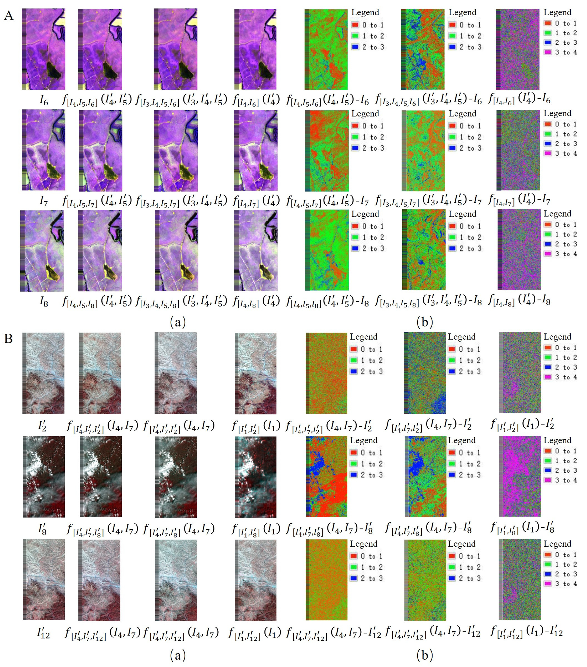
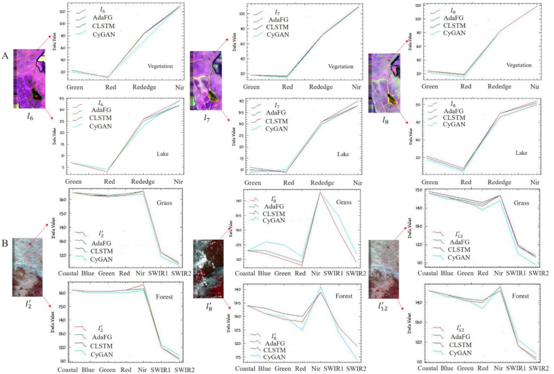
	$f_{\left[I_1^{\prime },I_{12}^{\prime }\right]}\left(I_1\right)$		2.796	2.629

shows the quantitative evaluation indicator between the generated result and reference image in the first aspect. The table shows that the entropy value produced by using the AdaFG network was higher than that using other networks, and the RMSE [36] value produced by using the AdaFG network was lower than that using other networks in both datasets. Figure 8 shows the visual effect and pixel error between the generated result and reference image using different networks in both datasets and illustrates that the generated result using different networks was close to the reference image. Figure 9 shows the spectral curves between the generated result and reference image using different networks at different coordinates (vegetation, lake, grass, forest) and illustrates that using different networks could maintain better spectral features between the generated result and the reference image in both datasets.

3.3.2. Single Network Datasets

In the second aspect, we constructed single network datasets according to the characteristics of different deep convolutions networks and existing images in both datasets. There were no reference images in this aspect. Figure 10 shows the generated results of UAV images using the AdaFG network from 2017 to 2019 and the visual effects of three-level generation according to the construction strategy in Table 3. Figure 11 shows the generated results of Landsat-8 images using the CyGAN network from 2013 to 2015 and the visual effects of two-level generation according to the construction strategy in Table 4. It appears that as the level of generation increased, the spectral features of the generated result became worse. This may be caused by the propagation of pixel error as the level of generation increased.

3.3.3. Multiple Network Datasets

In the third aspect, we constructed multiple network datasets to reduce the pixel error of the generated result caused by a single network. There were no reference images in this aspect. Figure 12 shows the generated results of UAV images using AdaFG, CLSTM, and CyGAN network from 2017 to 2019 and the visual effects of the generated results according to the construction strategy in Table 5. Figure 13 shows the generated results of Landsat-8 images using AdaFG, CLSTM, and CyGAN network from 2013 to 2015 and the visual effects of the generated results according to the construction strategy in Table 6. It appears that the visual effects of multiple network datasets are better than a single network.

3.3.4. Comparisons Between Single and Multiple Networks Datasets

In the second and third aspects, we conducted quantitative indicator evaluation between single network datasets and multiple network datasets.

Table 8. Quantitative evaluation indicator between the generated results using a single network (AdaFG, CyGAN) and multiple networks.

Datasets	Single Network	Multiple Network	Reference Images	RMSE (Pixel)
UAV	$f_{\left[I_4^{\prime },I_5^{\prime },I_{11}^{\prime }\right]}\left(I_4,I_5\right)$	$f_{\left[I_4^{\prime },I_{11}^{\prime }\right]}\left(I_4\right)$	$I_{11}^{″}$	4.953
				4.702
	$f_{\left[I_{10}^{\prime },I_{11}^{\prime },I_{12}^{\prime }\right]}\left(I_{10}^{″},I_{11}^{″}\right)$	$f_{\left[I_{10}^{\prime },I_{12}^{\prime }\right]}\left(I_{10}^{″}\right)$	$I_{12}^{\prime }$	3.847
				3.787
	$f_{\left[I_{10}^{\prime },I_{11}^{\prime },I_9^{\prime }\right]}\left(I_{10}^{″},I_{11}^{″}\right)$	$f_{\left[I_{10}^{\prime },I_{11}^{\prime },I_9^{\prime }\right]}\left(I_{10}^{″},I_{11}^{″}\right)$	$I_9^{\prime }$	2.723
				2.638
	$f_{\left[I_{10}^{\prime },I_{11}^{\prime },I_8^{\prime }\right]}\left(I_{10}^{″},I_{11}^{″}\right)$	$f_{\left[I_{10}^{\prime },I_{11}^{\prime },I_8^{\prime }\right]}\left(I_{10}^{″},I_{11}^{″}\right)$	$I_8$	2.879
				1.933
	$f_{\left[I_{10}^{\prime },I_{11}^{\prime },I_6^{\prime }\right]}\left(I_{10}^{″},I_{11}^{″}\right)$	$f_{\left[I_7^{\prime },\dots ,I_{12}^{\prime },I_6^{\prime }\right]}\left(I_7^{″},\dots ,I_{12}^{″}\right)$	$I_6$	3.483
				1.228
	$f_{\left[I_{10}^{\prime },I_{11}^{\prime },I_5^{\prime }\right]}\left(I_{10}^{″},I_{11}^{″}\right)$	$f_{\left[I_7^{\prime },\dots ,I_{12}^{\prime },I_5^{\prime }\right]}\left(I_7^{″},\dots ,I_{12}^{″}\right)$	$I_5^{\prime }$	2.967
				1.304
	$f_{\left[I_{10}^{\prime },I_{11}^{\prime },I_4^{\prime }\right]}\left(I_{10}^{″},I_{11}^{″}\right)$	$f_{\left[I_7^{\prime },\dots ,I_{12}^{\prime },I_4^{\prime }\right]}\left(I_7^{″},\dots ,I_{12}^{″}\right)$	$I_4^{\prime }$	3.100
				1.664
	$f_{\left[I_{10}^{\prime },I_{11}^{\prime },I_3^{\prime }\right]}\left(I_{10}^{″},I_{11}^{″}\right)$	$f_{\left[I_7^{\prime },\dots ,I_{12}^{\prime },I_3^{\prime }\right]}\left(I_7^{″},\dots ,I_{12}^{″}\right)$	$I_3$	3.864
				2.704
	$f_{\left[I_{10}^{\prime },I_{11}^{\prime },I_2^{\prime }\right]}\left(I_{10}^{″},I_{11}^{″}\right)$	$f_{\left[I_7^{\prime },\dots ,I_{12}^{\prime },I_2^{\prime }\right]}\left(I_7^{″},\dots ,I_{12}^{″}\right)$	$I_2^{\prime }$	3.504
				1.580
	$f_{\left[I_{10}^{\prime },I_{11}^{\prime },I_1^{\prime }\right]}\left(I_{10}^{″},I_{11}^{″}\right)$	$f_{\left[I_7^{\prime },\dots ,I_{12}^{\prime },I_1^{\prime }\right]}\left(I_7^{″},\dots ,I_{12}^{″}\right)$	$I_1$	3.188
				2.377
Landsat-8	$f_{\left[I_1^{\prime },I_2^{\prime }\right]}\left(I_1\right)$	$f_{\left[I_4^{\prime },I_7^{\prime },I_2^{\prime }\right]}\left(I_4,I_7\right)$	$I_2^{\prime }$	2.695
				1.144
	$f_{\left[I_1^{\prime },I_8^{\prime }\right]}\left(I_1\right)$	$f_{\left[I_4^{\prime },I_7^{\prime },I_8^{\prime }\right]}\left(I_4,I_7\right)$	$I_8^{\prime }$	5.017
				1.170
	$f_{\left[I_1^{\prime },I_{12}^{\prime }\right]}\left(I_1\right)$	$f_{\left[I_4^{\prime },I_7^{\prime },I_{12}^{\prime }\right]}\left(I_4,I_7\right)$	$I_{12}^{\prime }$	2.777
				0.929
	$f_{\left[I_1,I_3\right]}\left(I_1^{\prime }\right)$	$f_{\left[I_4,I_7,I_3\right]}\left(I_4^{\prime },I_7^{\prime }\right)$	$I_3$	2.632
				1.286
	$f_{\left[I_1,I_5\right]}\left(I_1^{\prime }\right)$	$f_{\left[I_4,I_7,I_5\right]}\left(I_4^{\prime },I_7^{\prime }\right)$	$I_5$	3.375
				1.411
	$f_{\left[I_1,I_{10}\right]}\left(I_1^{\prime }\right)$	$f_{\left[I_4,I_7,I_{10}\right]}\left(I_4^{\prime },I_7^{\prime }\right)$	$I_{10}$	3.990
				1.968
	$f_{\left[I_{12}^{\prime },I_8^{\prime }\right]}\left(I_{12}^{″}\right)$	$f_{\left[I_{11}^{\prime },I_{12}^{\prime },I_8^{\prime }\right]}\left(I_{11}^{″},I_{12}^{″}\right)$	$I_8^{\prime }$	5.022
				1.841
	$f_{\left[I_{12}^{\prime },I_7^{\prime }\right]}\left(I_{12}^{″}\right)$	$f_{\left[I_{11}^{\prime },I_{12}^{\prime },I_7^{\prime }\right]}\left(I_{11}^{″},I_{12}^{″}\right)$	$I_7^{\prime }$	4.399
				1.729
	$f_{\left[I_{12}^{\prime },I_4^{\prime }\right]}\left(I_{12}^{″}\right)$	$f_{\left[I_5^{\prime },\dots ,I_8^{\prime },I_4^{\prime }\right]}\left(I_5^{″},\dots ,I_8^{″}\right)$	$I_4^{\prime }$	2.771
				1.313
	$f_{\left[I_{12}^{\prime },I_3^{\prime }\right]}\left(I_{12}^{″}\right)$	$f_{\left[I_5^{\prime },\dots ,I_8^{\prime },I_3^{\prime }\right]}\left(I_5^{″},\dots ,I_8^{″}\right)$	$I_3$	3.367
				2.140
	$f_{\left[I_{12}^{\prime },I_2^{\prime }\right]}\left(I_{12}^{″}\right)$	$f_{\left[I_5^{\prime },\dots ,I_8^{\prime },I_2^{\prime }\right]}\left(I_5^{″},\dots ,I_8^{″}\right)$	$I_2^{\prime }$	2.606
				2.122
	$f_{\left[I_{12}^{\prime },I_1^{\prime }\right]}\left(I_{12}^{″}\right)$	$f_{\left[I_5^{\prime },\dots ,I_8^{\prime },I_1^{\prime }\right]}\left(I_5^{″},\dots ,I_8^{″}\right)$	$I_1^{\prime }$	2.686
				2.629

shows the quantitative evaluation indicator between the generated results using a single network (AdaFG, CyGAN) and multiple networks. The table shows that the RMSE value produced by using a single network (AdaFG, CyGAN) was higher than that using multiple networks in both datasets.

4. Discussions

4.1. Separable Convolution Kernel Sizes

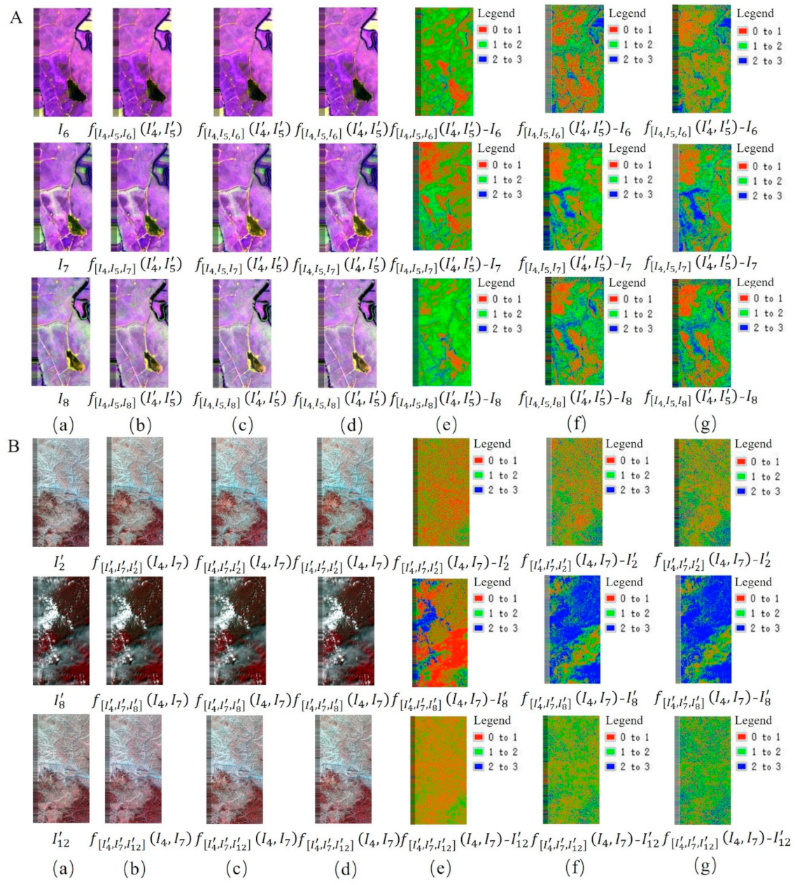
We observed that the separable convolution kernel size of the AdaFG network had an impact on the generated result, and conducted a visual comparison between the generated result and reference image using different separable convolution kernel sizes. We selected separable convolution kernels with sizes of 11, 13, and 15 to train the AdaFG network.

Table 9. Quantitative evaluation between the generated result and reference image using different separable convolution kernel sizes.

Datasets	Kernel Sizes	Generated Results	Reference Images	RMSE (Pixel)
UAV	11	$f_{\left[I_4,I_5,I_6\right]}\left(I_4^{\prime },I_5^{\prime }\right)$	$I_6$	1.128
		$f_{\left[I_4,I_5,I_7\right]}\left(I_4^{\prime },I_5^{\prime }\right)$	$I_7$	0.952
		$f_{\left[I_4,I_5,I_8\right]}\left(I_4^{\prime },I_5^{\prime }\right)$	$I_8$	0.954
	13	$f_{\left[I_4,I_5,I_6\right]}\left(I_4^{\prime },I_5^{\prime }\right)$	$I_6$	1.437
		$f_{\left[I_4,I_5,I_7\right]}\left(I_4^{\prime },I_5^{\prime }\right)$	$I_7$	1.273
		$f_{\left[I_4,I_5,I_8\right]}\left(I_4^{\prime },I_5^{\prime }\right)$	$I_8$	1.416
	15	$f_{\left[I_4,I_5,I_6\right]}\left(I_4^{\prime },I_5^{\prime }\right)$	$I_6$	1.444
		$f_{\left[I_4,I_5,I_7\right]}\left(I_4^{\prime },I_5^{\prime }\right)$	$I_7$	1.560
		$f_{\left[I_4,I_5,I_8\right]}\left(I_4^{\prime },I_5^{\prime }\right)$	$I_8$	1.418
Landsat-8	11	$f_{\left[I_4^{\prime },I_7^{\prime },I_2^{\prime }\right]}\left(I_4,I_7\right)$	$I_2^{\prime }$	1.144
		$f_{\left[I_4^{\prime },I_7^{\prime },I_8^{\prime }\right]}\left(I_4,I_7\right)$	$I_8^{\prime }$	1.170
		$f_{\left[I_4^{\prime },I_7^{\prime },I_{12}^{\prime }\right]}\left(I_4,I_7\right)$	$I_{12}^{\prime }$	0.929
	13	$f_{\left[I_4^{\prime },I_7^{\prime },I_2^{\prime }\right]}\left(I_4,I_7\right)$	$I_2^{\prime }$	1.689
		$f_{\left[I_4^{\prime },I_7^{\prime },I_8^{\prime }\right]}\left(I_4,I_7\right)$	$I_8^{\prime }$	2.533
		$f_{\left[I_4^{\prime },I_7^{\prime },I_{12}^{\prime }\right]}\left(I_4,I_7\right)$	$I_{12}^{\prime }$	1.402
	15	$f_{\left[I_4^{\prime },I_7^{\prime },I_2^{\prime }\right]}\left(I_4,I_7\right)$	$I_2^{\prime }$	1.938
		$f_{\left[I_4^{\prime },I_7^{\prime },I_8^{\prime }\right]}\left(I_4,I_7\right)$	$I_8^{\prime }$	2.875
		$f_{\left[I_4^{\prime },I_7^{\prime },I_{12}^{\prime }\right]}\left(I_4,I_7\right)$	$I_{12}^{\prime }$	1.633

shows the quantitative evaluation indicator and Figure 14 the visual effect and pixel error between the generated result and reference image using different separable convolution kernel sizes.

4.2. Stacked CLSTM Network Layers

We observed that the number of stacked CLSTM network layers had an impact on the generated result, and conducted a visual comparison between the generated result and reference image using different stacked CLSTM network layers. We selected 1 × 1, 2 × 2, and 3 × 3 stacked CLSTM network layers to train the CLSTM network.

Table 10. Quantitative evaluation between the generated result and reference image using different stacked CLSTM network layers.

Datasets	Stacked Numbers	Generated Results	Reference Images	RMSE (Pixel)
UAV	1 × 1	$f_{\left[I_3,I_4,I_5,I_6\right]}\left(I_3^{\prime },I_4^{\prime },I_5^{\prime }\right)$	$I_6$	2.681
		$f_{\left[I_3,I_4,I_5,I_7\right]}\left(I_3^{\prime },I_4^{\prime },I_5^{\prime }\right)$	$I_7$	2.096
		$f_{\left[I_3,I_4,I_5,I_8\right]}\left(I_3^{\prime },I_4^{\prime },I_5^{\prime }\right)$	$I_8$	2.186
	2 × 2	$f_{\left[I_3,I_4,I_5,I_6\right]}\left(I_3^{\prime },I_4^{\prime },I_5^{\prime }\right)$	$I_6$	1.976
		$f_{\left[I_3,I_4,I_5,I_7\right]}\left(I_3^{\prime },I_4^{\prime },I_5^{\prime }\right)$	$I_7$	1.556
		$f_{\left[I_3,I_4,I_5,I_8\right]}\left(I_3^{\prime },I_4^{\prime },I_5^{\prime }\right)$	$I_8$	1.617
	3 × 3	$f_{\left[I_3,I_4,I_5,I_6\right]}\left(I_3^{\prime },I_4^{\prime },I_5^{\prime }\right)$	$I_6$	1.758
		$f_{\left[I_3,I_4,I_5,I_7\right]}\left(I_3^{\prime },I_4^{\prime },I_5^{\prime }\right)$	$I_7$	1.300
		$f_{\left[I_3,I_4,I_5,I_8\right]}\left(I_3^{\prime },I_4^{\prime },I_5^{\prime }\right)$	$I_8$	1.421
Landsat-8	1 × 1	$f_{\left[I_4^{\prime },I_7^{\prime },I_2^{\prime }\right]}\left(I_4,I_7\right)$	$I_2^{\prime }$	2.265
		$f_{\left[I_4^{\prime },I_7^{\prime },I_8^{\prime }\right]}\left(I_4,I_7\right)$	$I_8^{\prime }$	3.386
		$f_{\left[I_4^{\prime },I_7^{\prime },I_{12}^{\prime }\right]}\left(I_4,I_7\right)$	$I_{12}^{\prime }$	1.935
	2 × 2	$f_{\left[I_4^{\prime },I_7^{\prime },I_2^{\prime }\right]}\left(I_4,I_7\right)$	$I_2^{\prime }$	1.780
		$f_{\left[I_4^{\prime },I_7^{\prime },I_8^{\prime }\right]}\left(I_4,I_7\right)$	$I_8^{\prime }$	2.697
		$f_{\left[I_4^{\prime },I_7^{\prime },I_{12}^{\prime }\right]}\left(I_4,I_7\right)$	$I_{12}^{\prime }$	1.577
	3 × 3	$f_{\left[I_4^{\prime },I_7^{\prime },I_2^{\prime }\right]}\left(I_4,I_7\right)$	$I_2^{\prime }$	1.537
		$f_{\left[I_4^{\prime },I_7^{\prime },I_8^{\prime }\right]}\left(I_4,I_7\right)$	$I_8^{\prime }$	1.681
		$f_{\left[I_4^{\prime },I_7^{\prime },I_{12}^{\prime }\right]}\left(I_4,I_7\right)$	$I_{12}^{\prime }$	1.484

shows the quantitative evaluation indicator and Figure 15 the visual effect and pixel error between the generated result and reference image using different stacked CLSTM network layers.

4.3. Proportional Hyper-Parameters

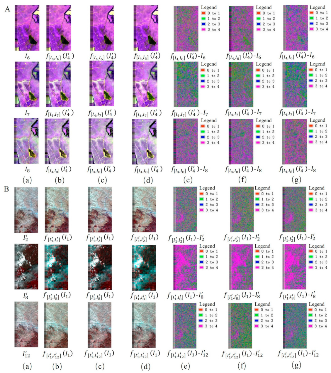
We observed that the proportional hyper-parameters of the CyGAN network had an impact on the generated result, and conducted a visual comparison between the generated result and reference image using different proportional hyper-parameters. We selected ${\mu }_1=250,{\mu }_2=1/16$, ${\mu }_1=350, {\mu }_2=1/32$ and ${\mu }_1=450,{\mu }_2=1/64$ to train the CyGAN network.

Table 11. Quantitative evaluation between the generated result and reference image using different proportional hyper-parameters.

Datasets	${\mathit{\mu }}_1,{\mathit{\mu }}_2$	Generated Results	Reference Images	RMSE (Pixel)
UAV	250,1/16	$f_{\left[I_4,I_6\right]}\left(I_4^{\prime }\right)$	$I_6$	3.643
		$f_{\left[I_4,I_7\right]}\left(I_4^{\prime }\right)$	$I_7$	3.271
		$f_{\left[I_4,I_8\right]}\left(I_4^{\prime }\right)$	$I_8$	3.836
	350,1/32	$f_{\left[I_4,I_6\right]}\left(I_4^{\prime }\right)$	$I_6$	3.585
		$f_{\left[I_4,I_7\right]}\left(I_4^{\prime }\right)$	$I_7$	3.077
		$f_{\left[I_4,I_8\right]}\left(I_4^{\prime }\right)$	$I_8$	3.690
	450,1/64	$f_{\left[I_4,I_6\right]}\left(I_4^{\prime }\right)$	$I_6$	3.814
		$f_{\left[I_4,I_7\right]}\left(I_4^{\prime }\right)$	$I_7$	3.263
		$f_{\left[I_4,I_8\right]}\left(I_4^{\prime }\right)$	$I_8$	3.698
Landsat-8	250,1/16	$f_{\left[I_1^{\prime },I_2^{\prime }\right]}\left(I_1\right)$	$I_2^{\prime }$	2.824
		$f_{\left[I_1^{\prime },I_8^{\prime }\right]}\left(I_1\right)$	$I_8^{\prime }$	5.708
		$f_{\left[I_1^{\prime },I_{12}^{\prime }\right]}\left(I_1\right)$	$I_{12}^{\prime }$	2.875
	350,1/32	$f_{\left[I_1^{\prime },I_2^{\prime }\right]}\left(I_1\right)$	$I_2^{\prime }$	2.694
		$f_{\left[I_1^{\prime },I_8^{\prime }\right]}\left(I_1\right)$	$I_8^{\prime }$	5.017
		$f_{\left[I_1^{\prime },I_{12}^{\prime }\right]}\left(I_1\right)$	$I_{12}^{\prime }$	2.629
	450,1/64	$f_{\left[I_1^{\prime },I_2^{\prime }\right]}\left(I_1\right)$	$I_2^{\prime }$	2.695
		$f_{\left[I_1^{\prime },I_8^{\prime }\right]}\left(I_1\right)$	$I_8^{\prime }$	5.553
		$f_{\left[I_1^{\prime },I_{12}^{\prime }\right]}\left(I_1\right)$	$I_{12}^{\prime }$	2.777

shows the quantitative evaluation indicator and Figure 16 visual effect and pixel error between the generated result and reference image using different proportional hyper-parameters.

5. Conclusions

The paper provides a remote-sensing sequence image construction scheme that can transform spectral mapping estimation and pixel synthesis into an easier process of using different deep convolution networks to construct remote-sensing sequence datasets. The major conclusions of this paper can be summarized as follows:

(1) The proposed AdaFG model provides a new method of generating remote-sensing images, especially for high-spatial-resolution images. CLSTM and CyGAN models can make up for the shortcoming of the AdaFG network model, which only performs single-scene generation and is affected by the missing degree of sequence images. The models can better capture and simulate complex and diverse nonlinear spectral transformation between different temporal images, and get better-generated images based on the models.

(2) Using separable convolution kernel of size 11 in AdaFG network, stacks of 3 × 3 CLSTM network layer, and ${\mu }_1=$350, ${\mu }_2=$1/32 in CyGAN network lead to better-generated results. Experiments show that the deep convolution network models can be used to get generated images to fill in missing areas of sequence images and produce remote-sensing sequence datasets.

The proposed AdaFG model is an image transformation method based on triple samples according to its structure, and its structure uses an adaptive separable convolution kernel. The spectral transformation ability of this model is higher than CLSTM and CyGAN models. However, this method only performs single-scene generation and its results are affected by the missing degree of sequence images. The proposed CLSTM model is an image transformation method based on multi-tuple samples according to its structure, and its structure is single-step stacked prediction. This model can perform predictions based on the state information of the time-series data. However, its results are affected by the length and missing degree of sequence images. The proposed CyGAN model is an image transformation method based on two-tuple samples according to its structure, and its structure uses cycle-consistent strategy and variable proportional hyper-parameters. This model can perform bidirectional transformation between different pictures, and its generated results are not affected by the degree of missing sequence images. However, the spectral transformation ability of this method is weak and its results are affected by the noise degree of sequence images.

When constructing remote-sensing time-series image datasets, it is necessary to make full use of the advantages of different deep convolution networks. When the missing degree of the sequence is small, using AdaFG and CLSTM model constructs the construction of remote-sensing time-series image datasets. When the missing degree of the sequence is larger, using the CyGAN model constructs the construction of remote-sensing time-series image datasets. Regardless of the quality and missing degree of sequence images, it is necessary to use the AdaFG model for the construction of remote-sensing time-series image datasets. In future work, we will make full use of the advantages of different deep convolution networks to construct a larger area remote-sensing sequence datasets.

References

1. Guo, H.; Wang, L.; Liang, D. Big Earth Data from space: A new engine for Earth science. Sci. Bull. 2016, 61, 505–513. [Google Scholar] [CrossRef]
2. Vatsavai, R.R.; Ganguly, A.; Chandola, V.; Stefanidis, A.; Klasky, S.; Shekhar, S. Spatio-Temporal Data Mining in the Era of Big Spatial Data: Algorithms and Applications. In Proceedings of the 1st ACM SIGSPATIAL International Workshop on Analytics for Big Geospatial Data, Redondo Beach, CA, USA, 6 November 2012. [Google Scholar]
3. Li, R.; Zhang, X.; Liu, B. Review on Filtering and Reconstruction Algorithms of Remote Sensing Time Series Data. J. Remote Sens. 2009, 13, 335–341. [Google Scholar]
4. Seaquist, J.W.; Chappell, A.; Eklundh, L. Exploring and Improving NOAA AVHRR NDVI Image Quality for African Dry-lands. Geosci. Remote Sens. Symp. 2002, 4, 2006–2008. [Google Scholar]
5. Berterretche, M.; Hudak, A.T.; Cohen, W.B.; Maiersperger, T.K.; Gower, S.T.; Dungan, J. Comparison of regression and geostatistical methods for mapping Leaf Area Index (LAI) with Landsat ETM+ data over a boreal forest. Remote Sens. Environ. 2005, 96, 49–61. [Google Scholar] [CrossRef] [Green Version]
6. Bhattacharjee, S.; Mitra, P.; Ghosh, S.K. Spatial Interpolation to Predict Missing Attributes in GIS Using Semantic Kriging. IEEE Trans. Geosci. Remote Sens. 2013, 52, 4771–4780. [Google Scholar] [CrossRef]
7. Zhou, H.; Wang, N.; Huang, Y. Comparison and analysis of remotely sensed time series of reconstruction models at various intervals. J. Geo-Inf. Sci. 2016, 18, 1410–1417. [Google Scholar]
8. Chen, J.; Jönsson, P.; Tamura, M.; Gu, Z.; Matsushita, B.; Eklundh, L. A simple method for reconstructing a high-quality NDVI time-series dataset based on the Savitzky-Golay filter. Remote Sens. Environ. 2004, 91, 332–344. [Google Scholar] [CrossRef]
9. Hua, D.; Yu, H. Objective Evaluation Method for Image Enhancement Quality Based on Visual Information Fidelity. Micro-Comput. Inf. 2012, 28, 173–175. [Google Scholar]
10. Crosson, W.L.; Al-Hamdan, M.Z.; Hemmings, S.N.; Wade, G.M. A daily merged MODIS Aqua-Terra land surface temperature dataset for the conterminous United States. Remote Sens. Environ. 2012, 119, 315–324. [Google Scholar] [CrossRef]
11. Hao, G.; Wu, B.; Zhang, L.; Fu, D.; Li, Y. Application and Analysis of ESTARFM Model in spatio-temporal Variation of Serincuo Lake Area, Tibet (1976–2014). J. Geo-Inf. Sci. 2016, 18, 833–846. [Google Scholar]
12. Peng, J.; Luo, W.; Ning, X.; Zou, Z. Fusion of remote sensing images based on the STARFM model. Cent. South For. Surv. Plan. 2018, 37, 32–37. [Google Scholar] [CrossRef]
13. Wang, Q.; Tang, Y.; Tong, X.; Atkinson, P.M. Virtual image pair-based spatio-temporal fusion. Remote Sens. Environ. 2020, 249, 112009. [Google Scholar] [CrossRef]
14. Xu, W.; Chen, R.; Huang, B.; Zhang, X.; Liu, C. Single Image Super-Resolution Based on Global Dense Feature Fusion Convolutional Network. Sensors 2019, 19, 316. [Google Scholar] [CrossRef] [PubMed] [Green Version]
15. Lu, Y.; Liu, J.; Jin, S. Image Processing on Time Series. Crim. Technol. 2004, 2, 41–42. [Google Scholar] [CrossRef]
16. Yuval, M.; Alonso, I.; Eyal, G.; Tchernov, D.; Loya, Y.; Murillo, A.C.; Treibitz, T. Repeatable Semantic Reef-Mapping through Photogrammetry and Label-Augmentation. Remote Sens. 2021, 13, 659. [Google Scholar] [CrossRef]
17. Kalajdjieski, J.; Zdravevski, E.; Corizzo, R.; Lameski, P.; Kalajdziski, S.; Pires, I.M.; Garcia, N.M.; Trajkovik, V. Air Pollution Prediction with Multi-Modal Data and Deep Neural Networks. Remote Sens. 2020, 12, 4142. [Google Scholar] [CrossRef]
18. Wang, W.; Liu, X.; Mou, X. Data Augmentation and Spectral Structure Features for Limited Samples Hyperspectral Classification. Remote Sens. 2021, 13, 547. [Google Scholar] [CrossRef]
19. Long, G.; Kneip, L.; Alvarez, J.M.; Li, H.; Zhang, X.; Yu, Q. Learning Image Matching by Simply Watching Video. In Proceedings of the European Conference on Computer Vision, Amsterdam, The Netherlands, 11–14 October 2016. [Google Scholar] [CrossRef]
20. Liu, Z.; Yeh, R.; Tang, X.; Liu, Y.; Agarwala, A. Video Frame Synthesis Using Deep Voxel Flow. In Proceedings of the IEEE International Conference on Computer Vision, Venice, Italy, 22–29 October 2017. [Google Scholar] [CrossRef] [Green Version]
21. Niklaus, S.; Mai, L.; Liu, F. Video Frame Interpolation via Adaptive Convolution. In Proceedings of the IEEE Conference on Computer Vision and Pattern Recognition, Honolulu, HI, USA, 21–26 July 2017. [Google Scholar]
22. Pan, X.L.; Zhang, Z.; Jiang, T. Research on NDVI prediction method based on convolutional long short-term memory network. Geogr. Inf. World 2020, 27, 60–67. [Google Scholar]
23. Zhu, J.Y.; Park, T.; Isola, P. Unpaired Image-to-Image Translation Using Cycle-Consistent Adversarial Networks. In Proceedings of the IEEE International Conference on Computer Vision, Venice, Italy, 22–29 October 2017; IEEE Computer Society: Washington, DC, USA; pp. 2223–2232. [Google Scholar] [CrossRef] [Green Version]
24. Alvarez-Vanhard, E.; Houet, T.; Mony, C.; Lecoq, L.; Corpetti, T. Can UAVs fill the gap between in situ surveys and satellites for habitat mapping? Remote Sens. Environ. 2020, 243, 111780. [Google Scholar] [CrossRef]
25. Dong, C.; Loy, C.C.; He, K.; Tang, X. Image Super-Resolution Using Deep Convolutional Networks. IEEE Trans. Pattern Anal. Mach. Intell. 2015, 38, 295–307. [Google Scholar] [CrossRef] [PubMed] [Green Version]
26. Zeiler, M.D.; Taylor, G.W.; Fergus, R. Adaptive Deconvolutional Networks for Mid and High Level Feature Learning. In Proceedings of the 2011 International Conference on Computer Vision, Barcelona, Spain, 6–13 November 2011; pp. 2018–2025. [Google Scholar]
27. Shi, W.; Caballero, J.; Huszar, F.; Totz, J.; Aitken, A.P.; Bishop, R.; Rueckert, D.; Wang, Z. Real-Time Single Image and Video Super-Resolution Using an Efficient Sub-Pixel Convolutional Neural Network. In Proceedings of the 2016 IEEE Conference on Computer Vision and Pattern Recognition (CVPR), Las Vegas, NV, USA, 27–30 June 2016; pp. 1874–1883. [Google Scholar]
28. Bishop, C.M. Pattern Recognition and Machine Learning; Springer: New York, NY, USA, 2006. [Google Scholar]
29. Long, J.; Shelhamer, E.; Darrell, T. Fully Convolutional Networks for Semantic Segmentation. In Proceedings of the IEEE Conference on Computer Vision and Pattern Recognition, Boston, MA, USA, 7–12 June 2015; pp. 3431–3440. [Google Scholar]
30. Yuan, Z.; Zhou, X.; Yang, T. Hetero-ConvLSTM: A Deep Learning Approach to Traffic Accident Prediction on Heterogeneous Spatio-Temporal Data. In Proceedings of the International Conference on Knowledge Discovery & Data Mining, London, UK, 19–23 August 2018; pp. 984–992. [Google Scholar] [CrossRef]
31. Zhao, C.; Chen, P.H. Icon Shape Generation Based on Generative Adversarial Network. Comput. Sci. Appl. 2020, 10, 456–463. [Google Scholar] [CrossRef]
32. Tian, L.; Cao, Y.; He, B.; Zhang, Y.; He, C.; Li, D. Image Enhancement Driven by Object Characteristics and Dense Feature Reuse Network for Ship Target Detection in Remote Sensing Imagery. Remote Sens. 2021, 13, 1327. [Google Scholar] [CrossRef]
33. Lu, C.-G. A generalization of Shannon’s information theory. Int. J. Gen. Syst. 1999, 28, 453–490. [Google Scholar] [CrossRef]
34. Kingma, D.P.; Ba, J. Adam: A method for stochastic optimization. arXiv 2014, arXiv:1412.6980. [Google Scholar]
35. Collobert, R.; Kavukcuoglu, K.; Farabet, C. Torch7: A MatLab-Like Environment for Machine Learning. In BigLearn, NIPS Workshop; no.EPFL-CONF-192376; Granada, Spain, 1 January 2011; Available online: https://infoscience.epfl.ch/record/192376/ (accessed on 15 October 2020).
36. Huang, X.; Shi, J.; Yang, J.; Yao, J. Evaluation of Color Image Quality Based on Mean Square Error and Peak Signal-to-Noise Ratio of Color Difference. Acta Photonica Sin. 2007, S1, 295–298. Available online: http://en.cnki.com.cn/Article_en (accessed on 15 October 2020).
Figure 1. Location of unmanned aerial vehicle (UAV) dataset: 1, 2, 3 band composite.
Remotesensing 13 01853 g001
Figure 2. Location of Landsat-8 dataset: 5, 4, 3 band composite.
Remotesensing 13 01853 g002
Figure 3. Overview of AdaFG architecture: (ad) represent feature extracting part, feature expanding part, separable convolution part, and backpropagation part, respectively.
Remotesensing 13 01853 g003
Figure 4. Cell structure of CLSTM.
Remotesensing 13 01853 g004
Figure 5. Structure diagram of CyGAN: (a,b) show forward and backward cycle-consistent loss.
Remotesensing 13 01853 g005
Figure 6. Visual effect of training ( I t ) and testing ( I t ) images using different deep convolution networks in the first aspect: (A) UAV and (B) Landsat-8 images; (ac) show the visual effect using AdaFG, CLSTM, and CyGAN network, respectively.
Remotesensing 13 01853 g006
Figure 7. Strategy for constructing sequence datasets in the second and third aspect: (A) available UAV images from 2017 to 2019 and Landsat-8 images from 2013 to 2015; (B) one construction strategy with single network; (C) one construction strategy with multiple networks.
Remotesensing 13 01853 g007
Figure 8. (a) Visual effect and (b) pixel error between generated result and reference image using different deep convolution networks: (A) UAV and (B) Landsat-8 datasets.
Remotesensing 13 01853 g008
Figure 9. Spectral curves between generated result and reference image using different deep convolution networks at different coordinates: (A) UAV and (B) Landsat-8 datasets.
Remotesensing 13 01853 g009
Figure 10. Generated results of UAV images using AdaFG network from 2017 to 2019 according to construction strategy in Table 3: existing images and generated results in (A) 2019 sequence, (B) 2018 sequence, and (C) 2017 sequence.
Remotesensing 13 01853 g010
Figure 11. Generated results of Landsat-8 images using CyGAN network from 2013 to 2015 according to construction strategy in Table 4: existing images and generated results in (A) 2015 sequence, (B) 2014 sequence, and (C) 2013 sequence.
Remotesensing 13 01853 g011
Figure 12. Generated results of UAV images using AdaFG, CLSTM, and CyGAN network from 2017 to 2019 according to construction strategy in Table 5: existing images and generated results in (A) 2019 sequence, (B) 2018 sequence, and (C) 2017 sequence.
Remotesensing 13 01853 g012
Figure 13. Generated results of Landsat-8 images using AdaFG, CLSTM, and CyGAN network from 2013 to 2015 according to construction strategy in Table 6: existing images and generated results in (A) 2015 sequence, (B) 2014 sequence, and (C) 2013 sequence.
Remotesensing 13 01853 g013
Figure 14. (a) Initial image, (bd) Visual effect and (eg) pixel error between the generated results and reference image using separable convolution kernel sizes 11, 13, and 15: (A) UAV and (B) Landsat-8 datasets.
Remotesensing 13 01853 g014
Figure 15. (a) Initial image, (bd) Visual effect and (eg) pixel error between the generated result and reference image using stacks of 1 × 1, 2 × 2, and 3 × 3 CLSTM network layers: (A) UAV and (B) Landsat-8 datasets.
Remotesensing 13 01853 g015
Figure 16. (a) Initial image, (bd) Visual effect and (eg) pixel error between the generated result and reference image using different proportional hyper-parameters: (A) UAV and (B) Landsat-8 datasets.
Remotesensing 13 01853 g016