
Effect of 6-DOF Oscillation of Ship Target on SAR Imaging


Abstract
1. Introduction
- (1)
- The state-of-the-art researches concerning ship oscillation and SAR imaging are relatively dispersed, and there is no systematic description and derivation of the phase distortion introduced by ship 6-DOF oscillation;
- (2)
- The ship oscillation in most of the existing analyses are obtained through numerical simulation, and part of the conclusions lack the verification by measured attitude data.
2. Model of Oscillatory Ship Target
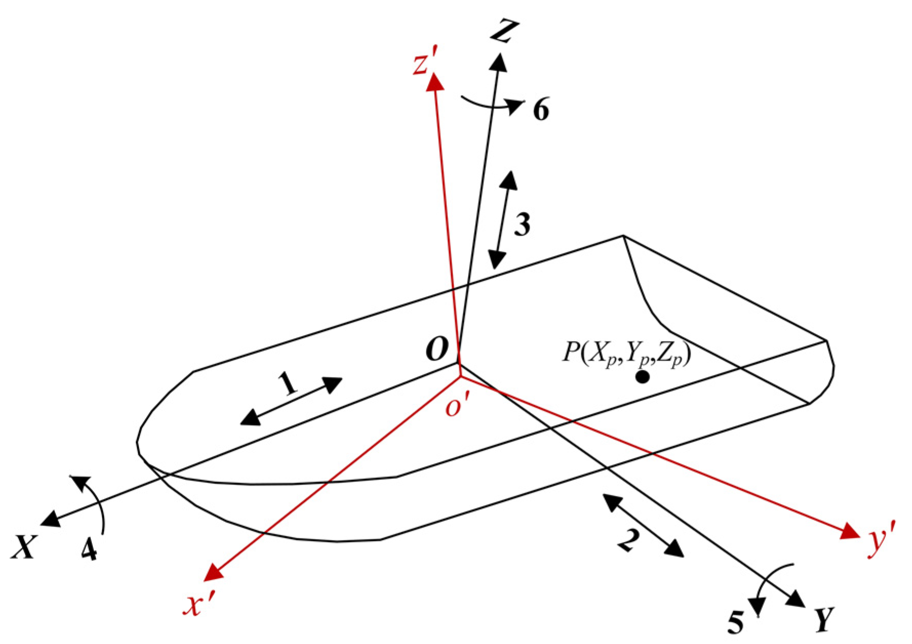
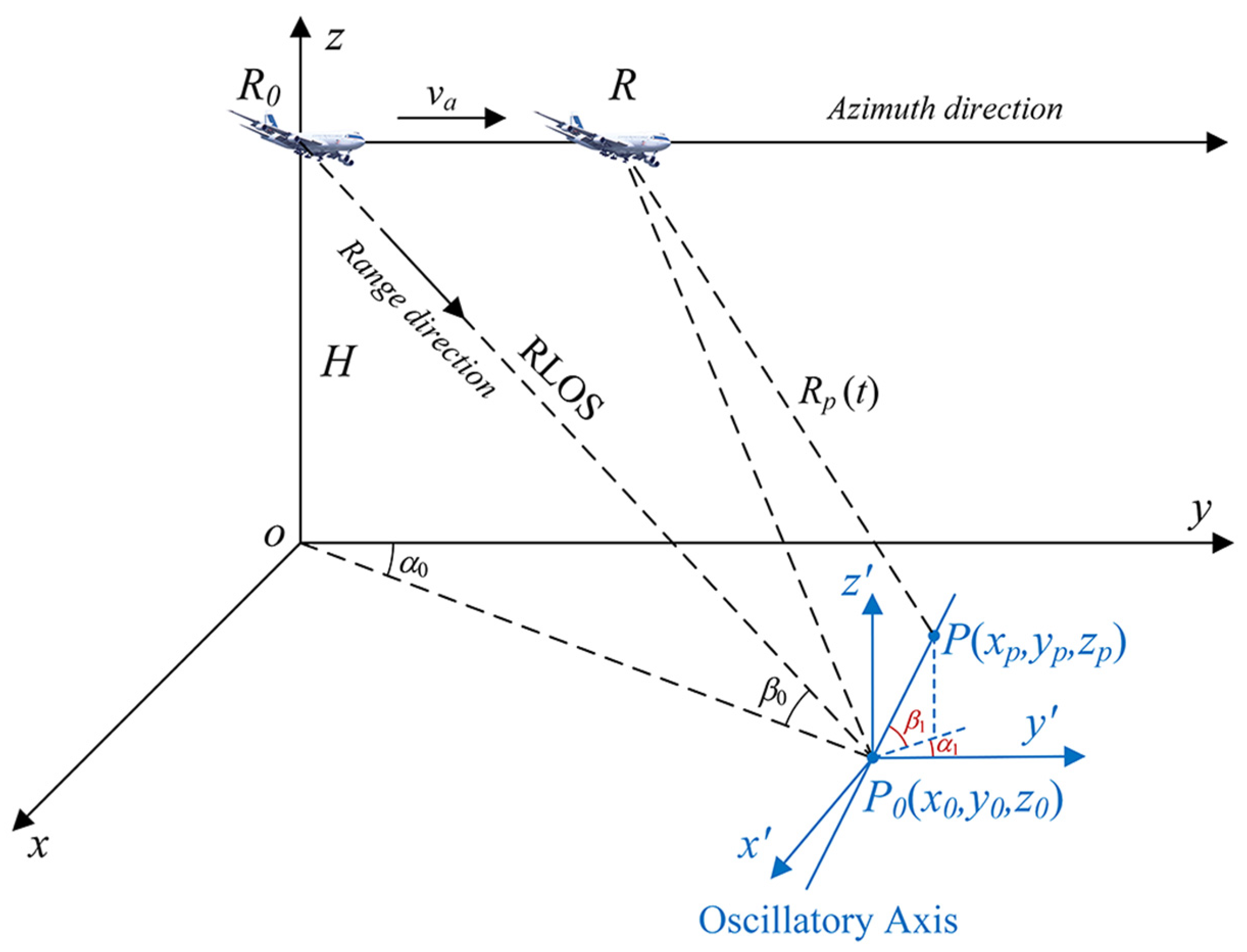
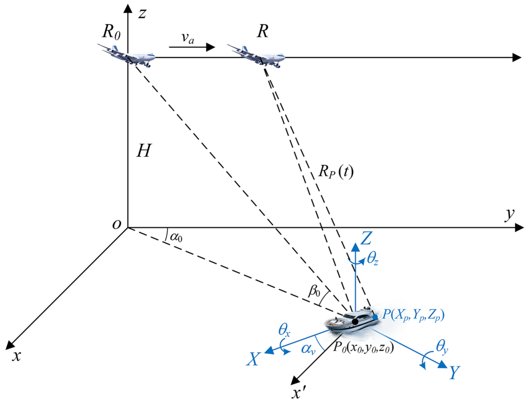
2.1. Range Model of a Ship Target Based on 6-DOF Motion
2.2. Ship Linear Oscillation
2.2.1. Single-Frequency Linear Oscillation
2.2.2. Multi-Frequency Linear Oscillation
2.3. Ship Angular Oscillation
2.3.1. Single-Frequency Angular Oscillation
- (1)
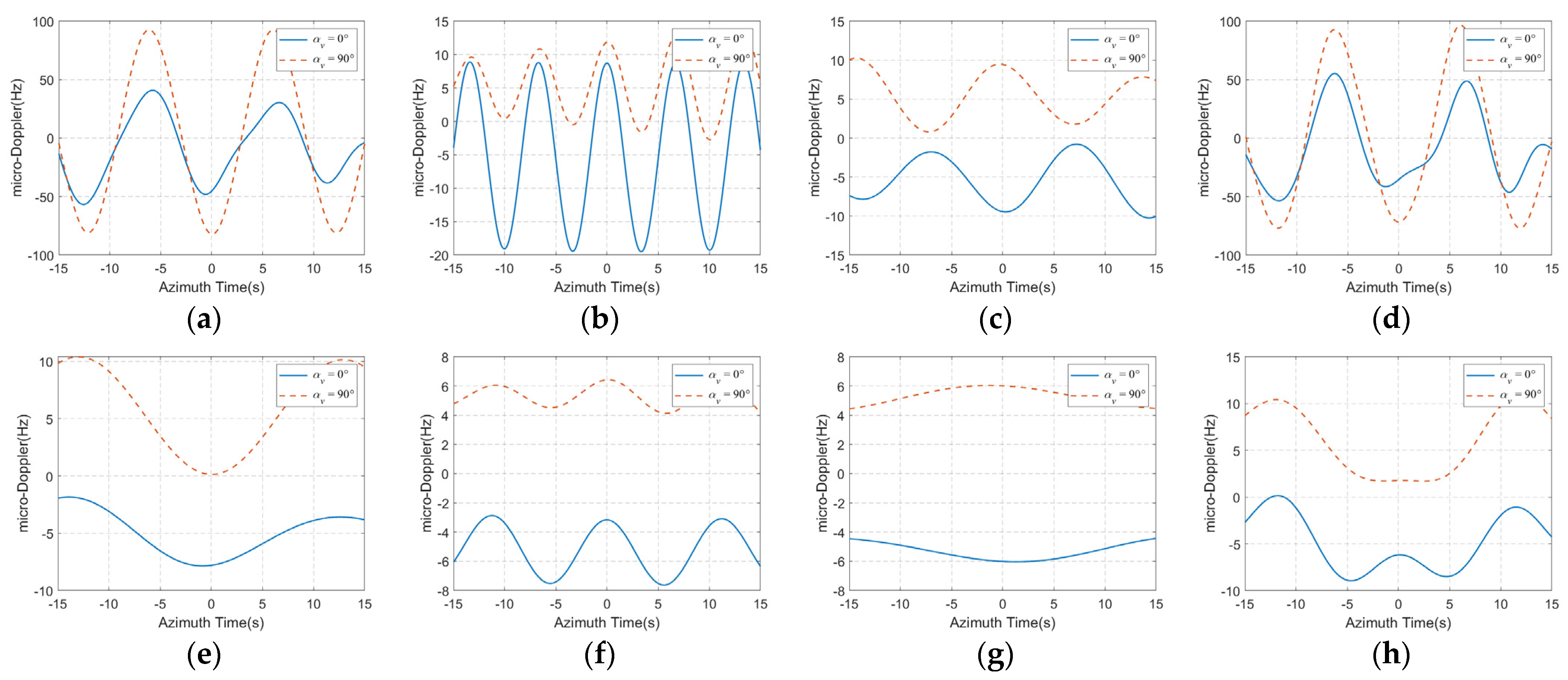
- Under the given coordinate (10 m, 10 m, 10 m), the magnitude of the micro-Doppler introduced by the three angular oscillations is . The roll motion seems to be dominant when the ship is small, and this dominance will gradually weaken as the ship size increases.
- (2)
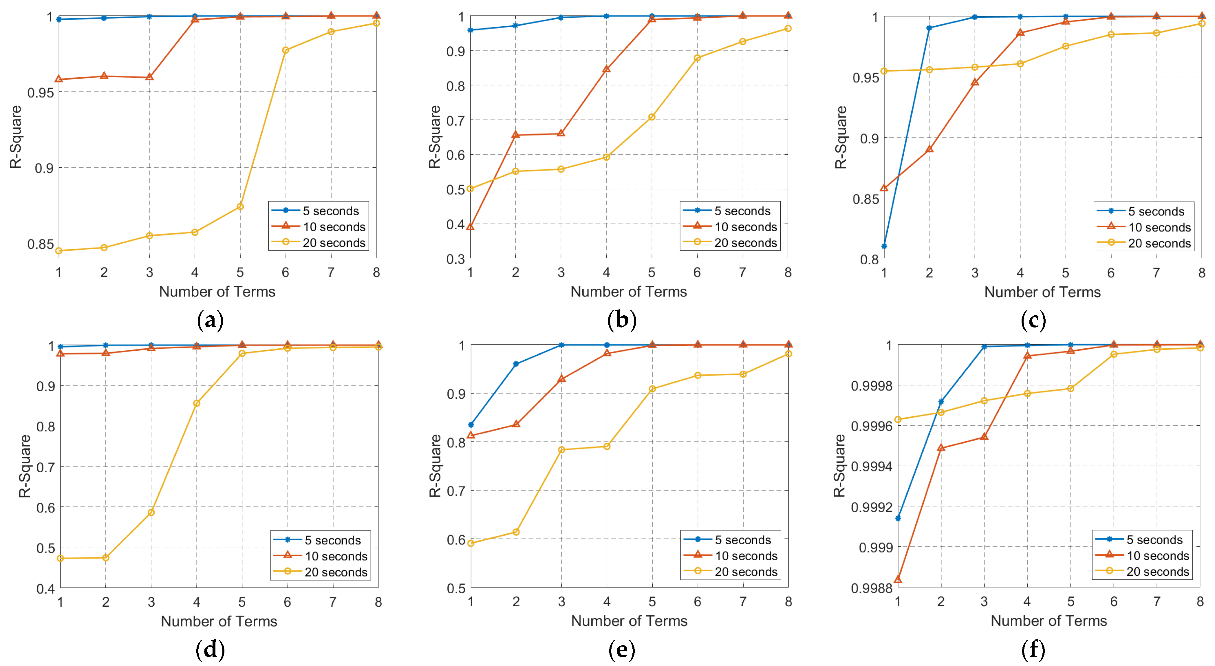
- When all the three angular oscillations exist at the same time, the micro-Doppler will become a relatively complex form, and the its periodicity will also be weakened, which may require more sinusoidal terms to better fit it.
- (3)
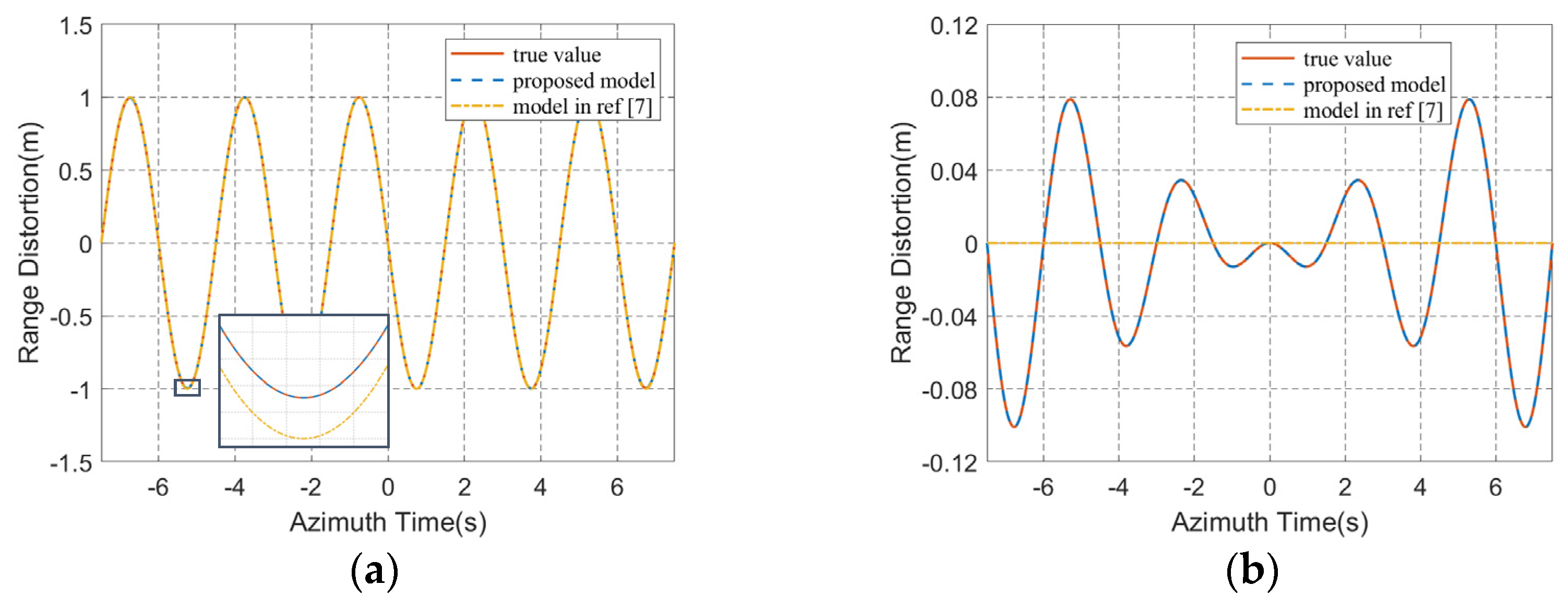
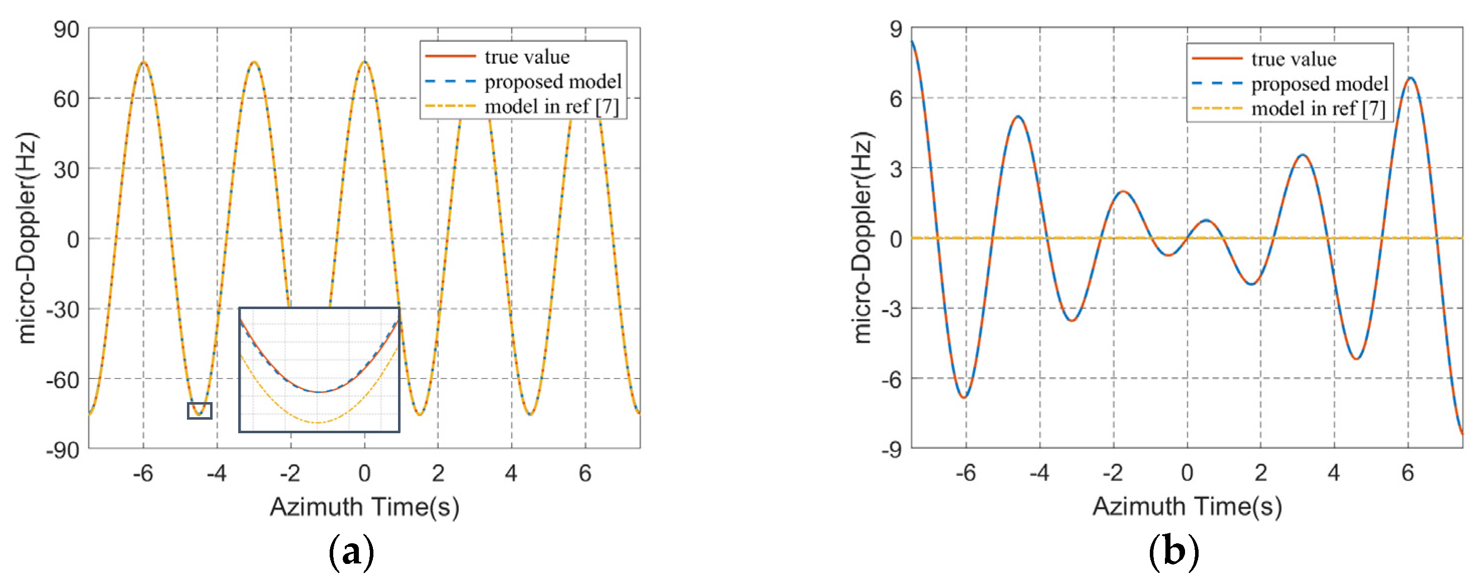
- With different heading angles, the micro-Doppler caused by angular oscillations has significant differences. According to Equation (33), the mean micro-Doppler introduced by roll motion is determined by . Bring the simulation parameters into this formula, when the heading angle is 0° and 90°, the mean micro-Doppler of point P introduced by carrier rolling is –5.45 Hz and 5.45 Hz, respectively. The calculation results agree well with simulation results in Figure 9e, which proves the validity of the proposed model.
2.3.2. Multi-Frequency Angular Oscillation
3. The Effect of Oscillation on Imaging
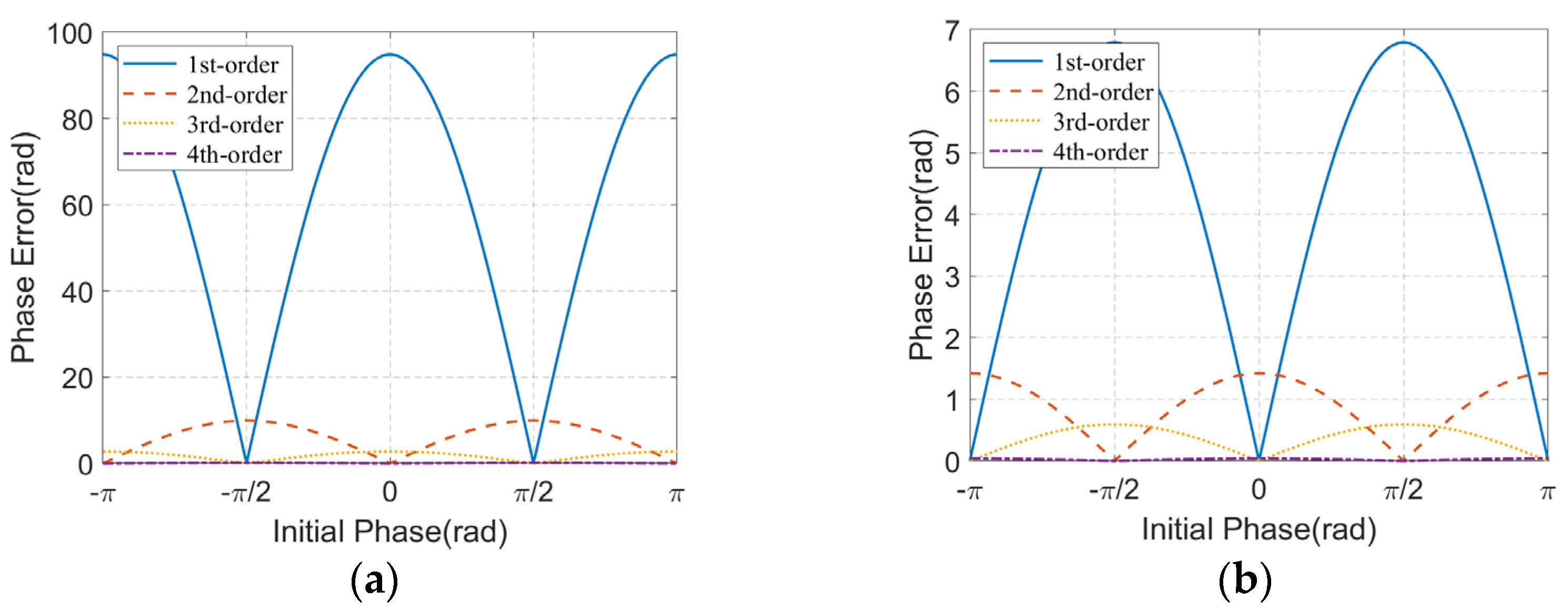
3.1. CPI Less Than the Oscillation Period
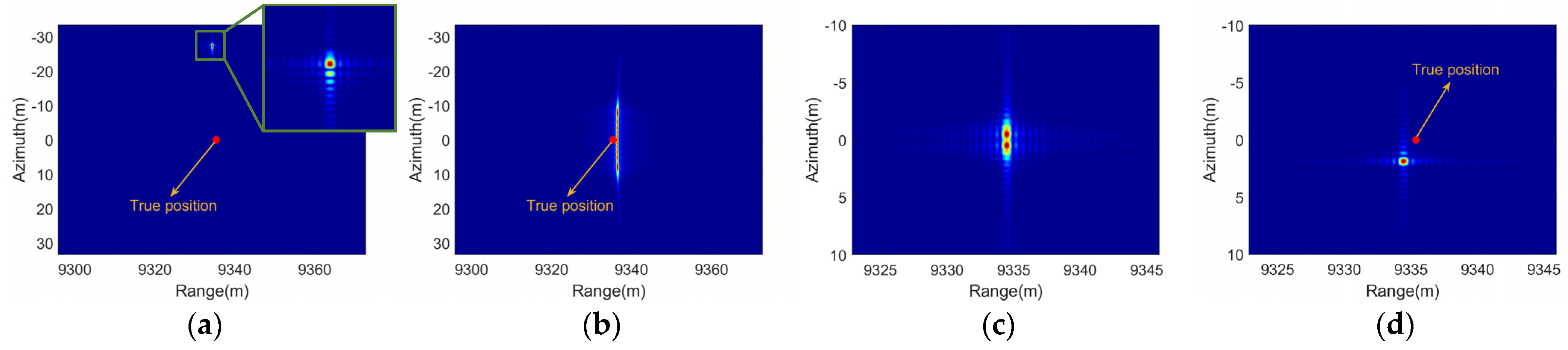
3.1.1. Ship Linear Oscillation
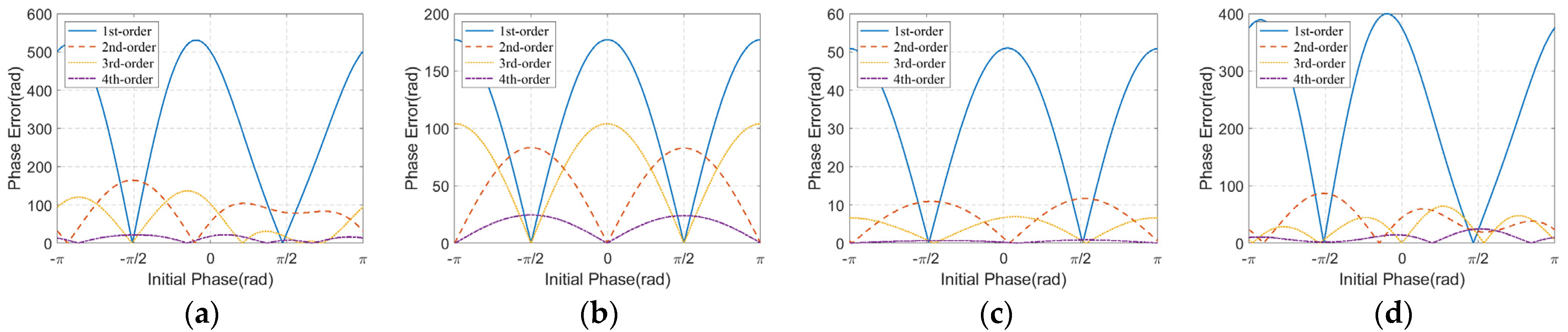
3.1.2. Ship Angular Oscillation
3.2. CPI Greater Than the Oscillation Period
3.2.1. Ship Linear Oscillation
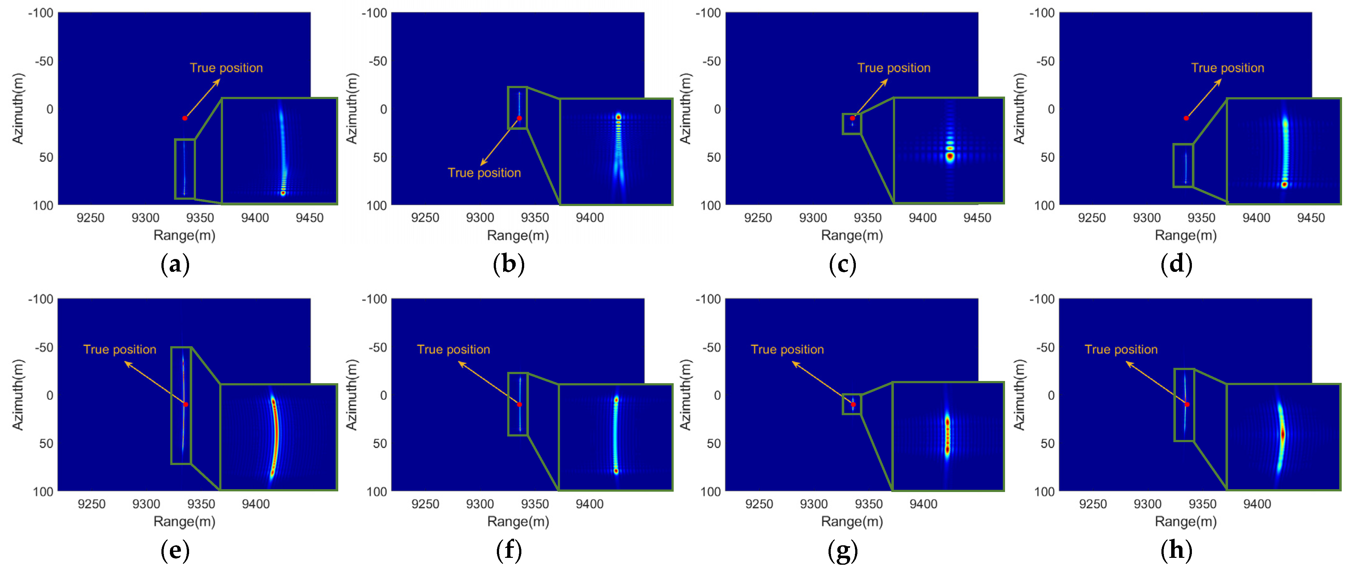
3.2.2. Ship Angular Oscillation
4. Measured Data and Experimental Results
4.1. Measured Data of Ship Attitude
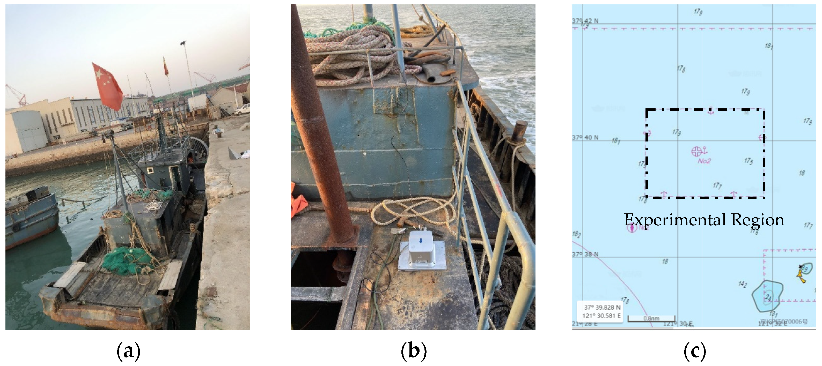
4.1.1. Experimental Condition
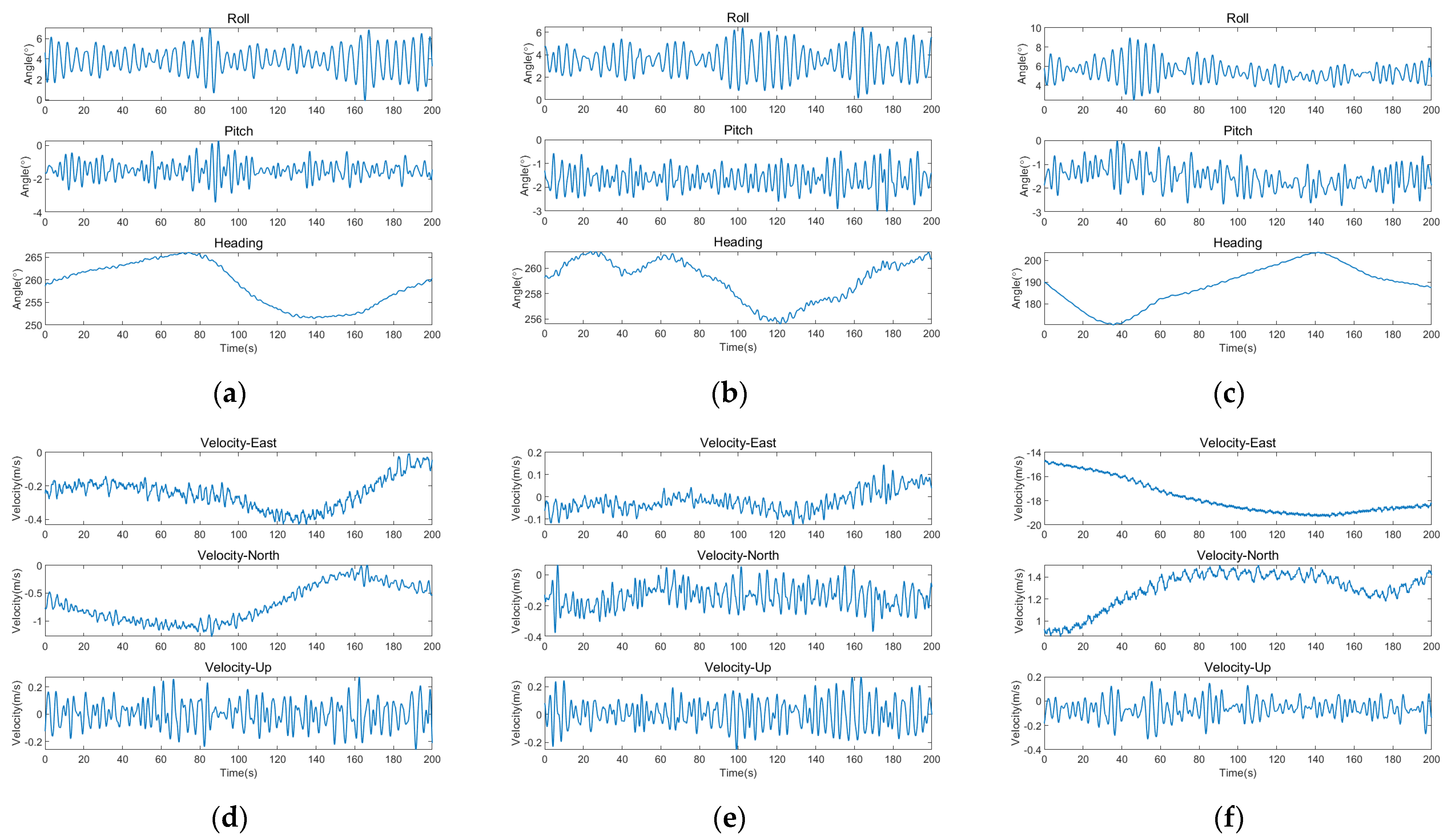
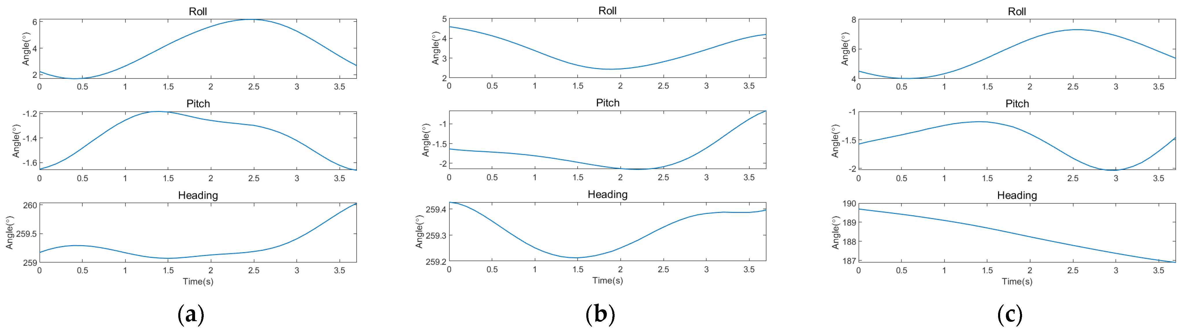
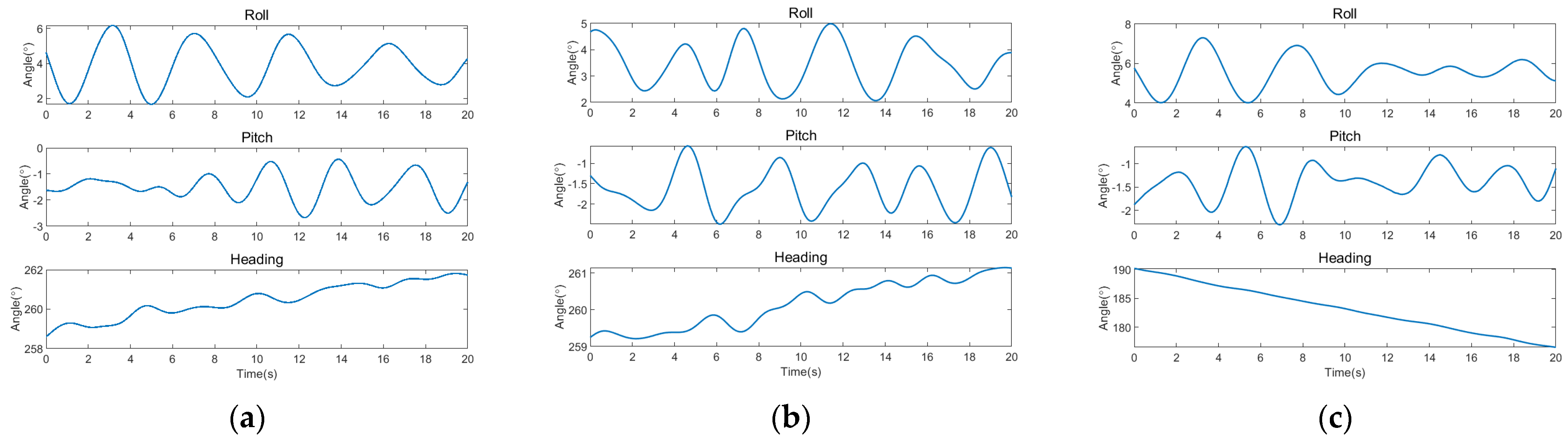
4.1.2. Measured Data
- (1)
- Set off from the harbor to experimental region;
- (2)
- Turned off the power and allowed the ship to drift along the current, then recorded the attitude data of the ship, this process lasted about 1.5 h;
- (3)
- Anchored the ship to the center of the anchorage, then recorded the attitude data of the ship, this process continued for 2 h;
- (4)
- Weighed anchor and drove the ship back-and-forth along a specific route, recorded the attitude data of the ship during this process, this step took about 40 min;
- (5)
- Back to the harbor.
4.2. Experiments Based on the Measured Attitude Data
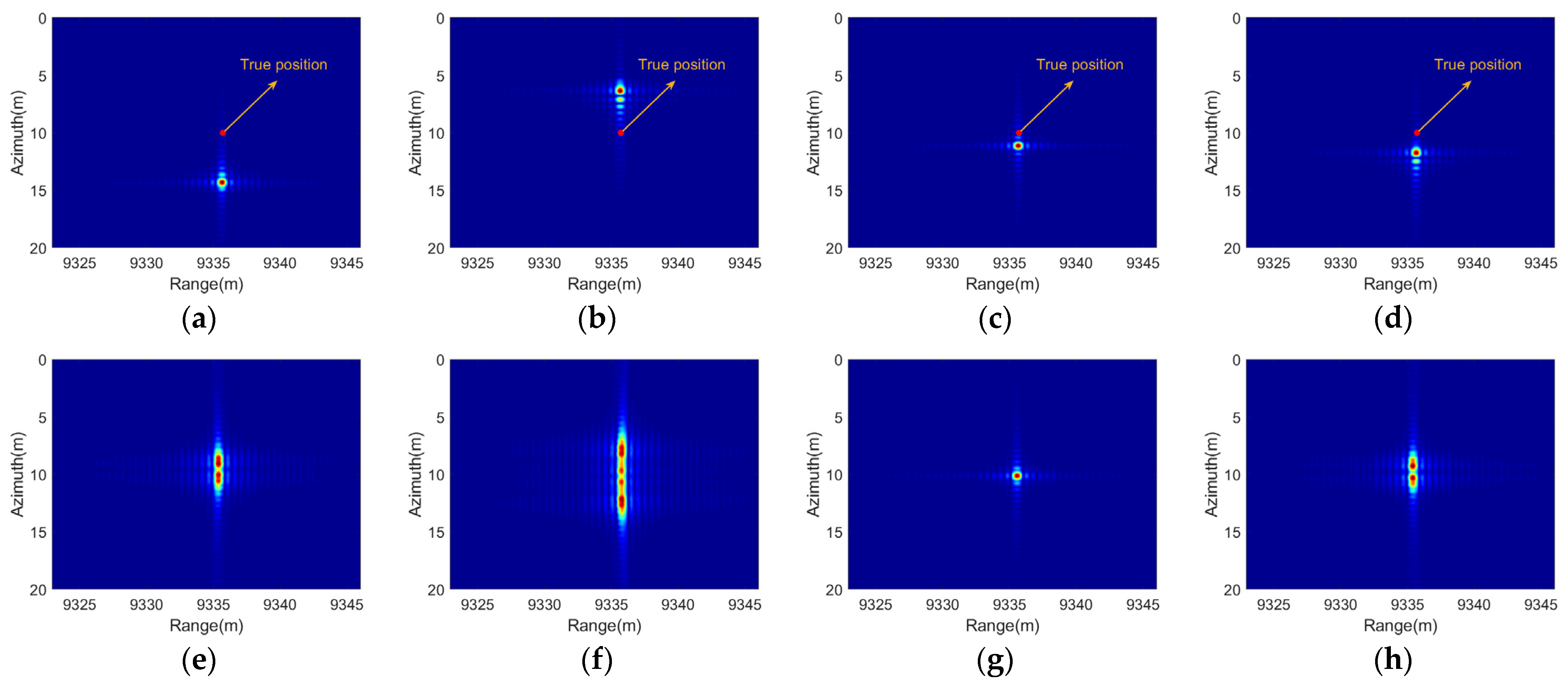
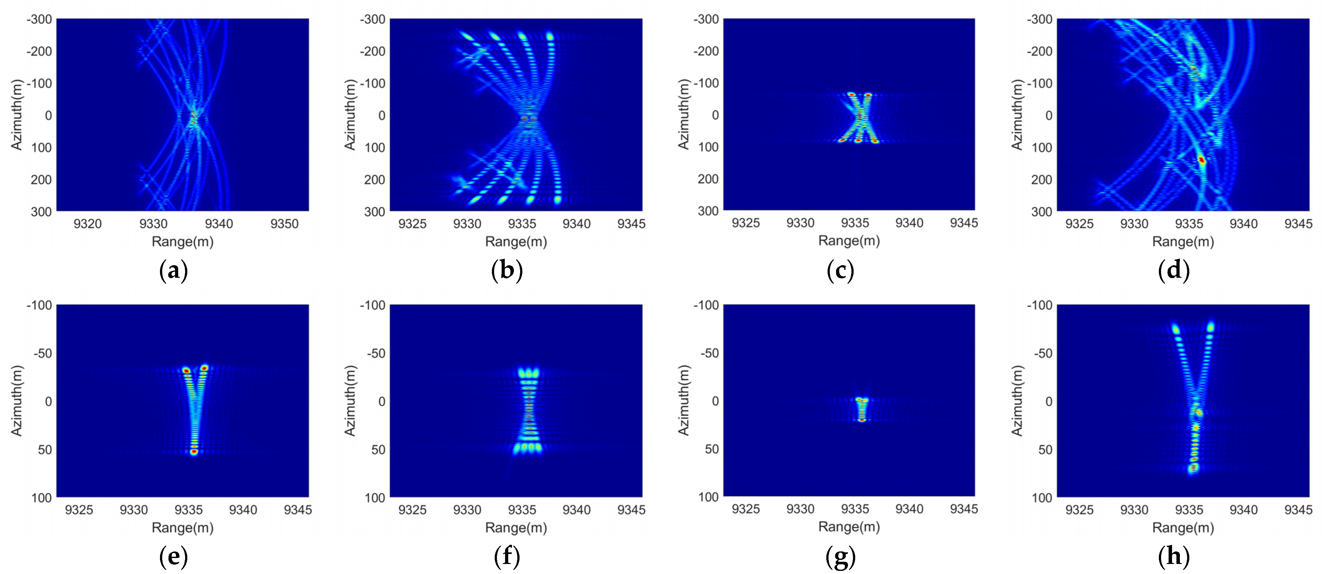
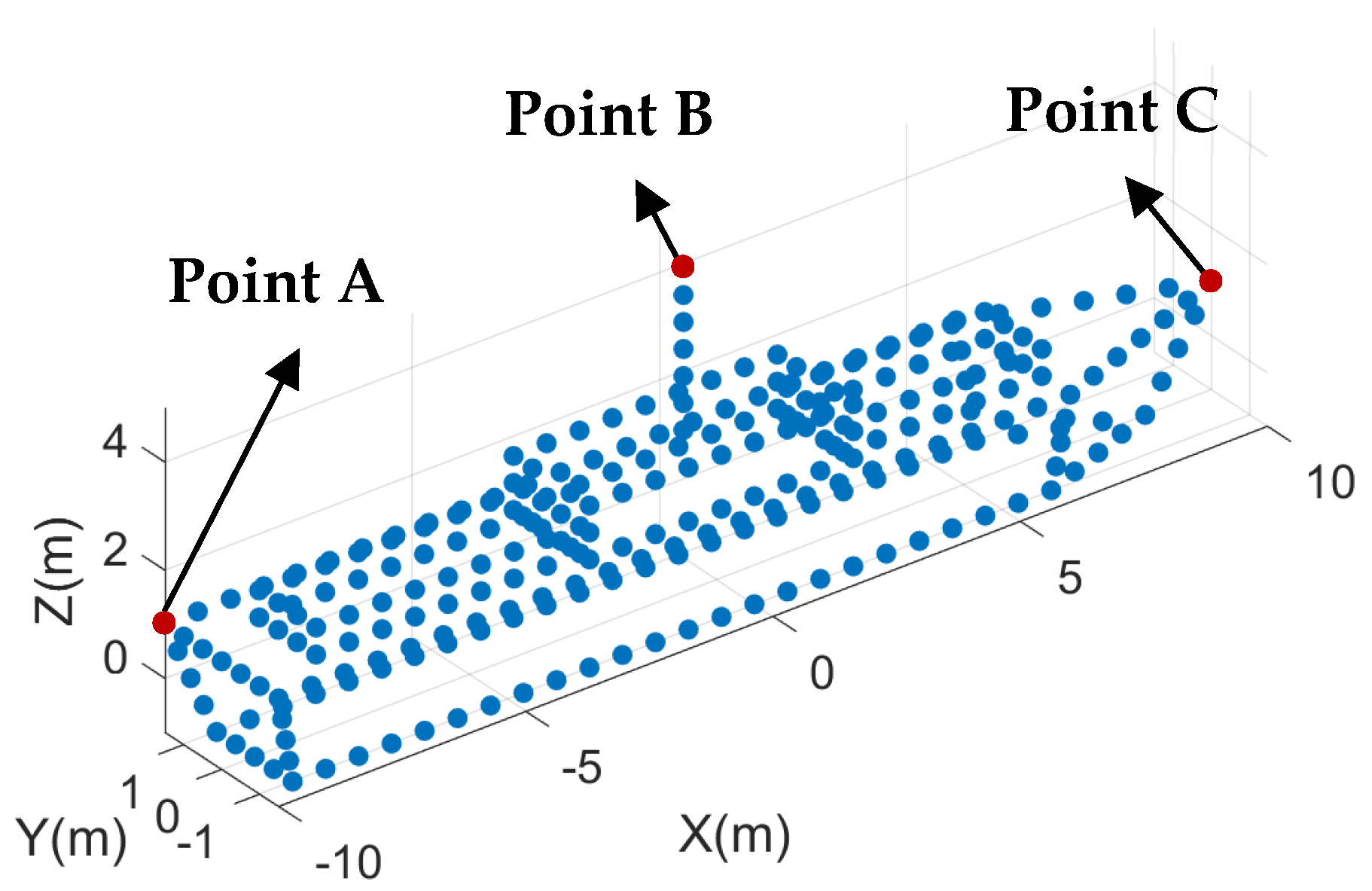
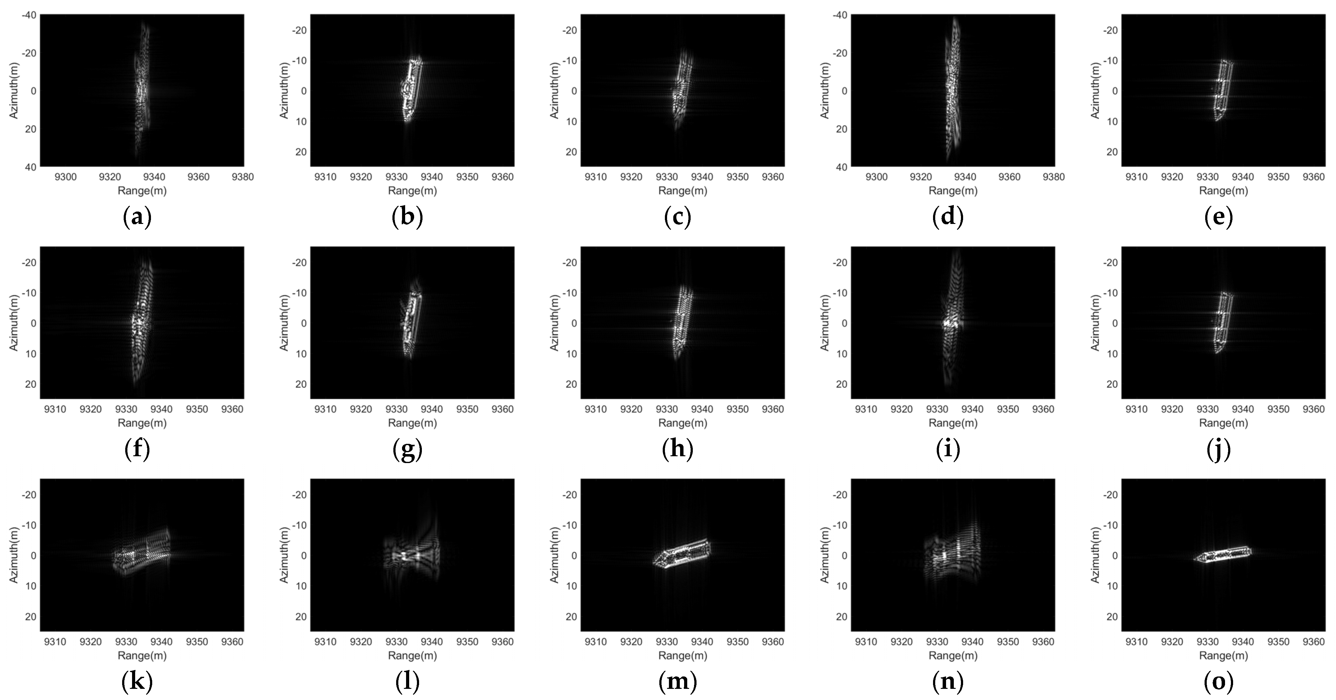
4.2.1. Focusing Results of the Oscillatory Ship
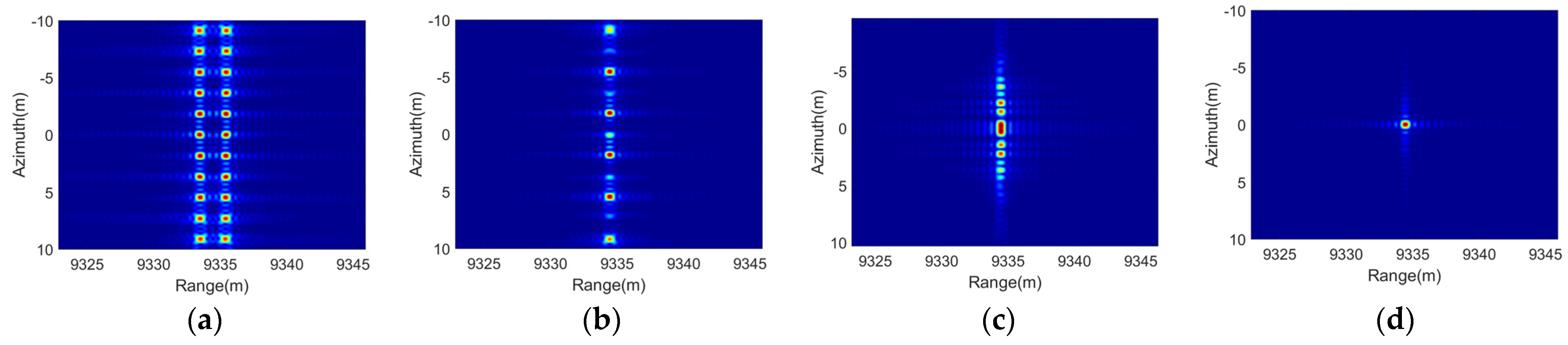
4.2.2. Phase Compensation Based on the Proposed Range Model
- (1)
- verifying the accuracy of the proposed range model for ship angular oscillation;
- (2)
- exploring the feasibility of phase compensation by fitting ship attitude angles with multi-frequency oscillation model.
5. Conclusions
Author Contributions
Funding
Acknowledgments
Conflicts of Interest
Appendix A. The Specific Derivation Result of Range Distortion When Roll, Pitch, and Yaw Motion All Exist
Appendix B. The Range Distortion and micro-Doppler Introduced by Pitch and Yaw
References
- Cumming, I.; Wong, F. Digital Processing of Synthetic Aperture Radar Data: Algorithms and Implementation; Artech House: Boston, MA, USA, 2005; pp. 113–168. [Google Scholar]
- Vessel Motion Calculator. Available online: https://calqlata.com/productpages/00059-help.html (accessed on 16 February 2021).
- Yao, G.; Xie, J.; Huang, W. Ocean Surface Cross Section for Bistatic HF Radar Incorporating a Six DOF Oscillation Motion Model. Remote Sens. 2019, 11, 2738. [Google Scholar] [CrossRef]
- Yao, G.; Xie, J.; Huang, W. HF Radar Ocean Surface Cross Section for the Case of Floating Platform Incorporating a Six-DOF Oscillation Motion Model. IEEE J. Ocean. Eng. 2021, 46, 156–171. [Google Scholar] [CrossRef]
- Ouchi, K.; Iehara, M.; Morimura, K.; Kumano, S.; Takami, I. Nonuniform azimuth image shift observed in the Radarsat images of ships in motion. IEEE Trans. Geosci. Remote Sens. 2002, 40, 2188–2195. [Google Scholar] [CrossRef]
- Doerry, A. Ship Dynamics for Maritime ISAR Imaging; No. SAND2008-1020; Sandia National Laboratories: Albuquerque, NM, USA, 2008. [Google Scholar]
- Li, X.; Deng, B.; Qin, Y.; Wang, H.; Li, Y. The influence of target micromotion on SAR and GMTI. IEEE Trans. Geosci. Remote Sens. 2011, 49, 2738–2751. [Google Scholar] [CrossRef]
- Liu, P.; Jin, Y. A study of ship rotation effects on SAR image. IEEE Trans. Geosci. Remote Sens. 2017, 55, 3132–3144. [Google Scholar] [CrossRef]
- Liu, W.; Sun, G.; Xia, X.; Fu, J.; Xing, M.; Bao, Z. Focusing Challenges of Ships with Oscillatory Motions and Long Coherent Processing Interval. IEEE Trans. Geosci. Remote Sens. 2020. [Google Scholar] [CrossRef]
- Biondi, F. COSMO-SkyMed Staring Spotlight SAR Data for Micro-Motion and Inclination Angle Estimation of Ships by Pixel Tracking and Convex Optimization. Remote Sens. 2019, 11, 766. [Google Scholar]
- Biondi, F.; Addabbo, P.; Orlando, D.; Clemente, C. Micro-Motion Estimation of Maritime Targets Using Pixel Tracking in Cosmo-Skymed Synthetic Aperture Radar Data—An Operative Assessment. Remote Sens. 2019, 11, 1637. [Google Scholar] [CrossRef]
- Xu, G.; Xing, M.; Xia, X.; Zhang, L.; Chen, Q.; Bao, Z. 3D Geometry and Motion Estimations of Maneuvering Targets for Interferometric ISAR With Sparse Aperture. IEEE Trans. Image Process. 2016, 25, 2005–2020. [Google Scholar] [CrossRef]
- Wang, F.; Xu, F.; Jin, Y. 3-D information of a space target retrieved from a sequence of high-resolution 2-D ISAR images. In Proceedings of the 2016 IEEE International Geoscience and Remote Sensing Symposium, Beijing, China, 10–15 July 2016; pp. 5000–5002. [Google Scholar]
- Ruegg, M.; Meier, E.; Nuesch, D. Vibration and rotation in millimeter-wave SAR. IEEE Trans. Geosci. Remote Sens. 2007, 45, 293–304. [Google Scholar] [CrossRef]
- Zhang, Y.; Sun, J.; Lei, P.; Hong, W. SAR-based paired echo focusing and suppression of vibrating targets. IEEE Trans. Geosci. Remote Sens. 2014, 52, 7593–7605. [Google Scholar] [CrossRef]
- Liu, Y.; Zhu, D.; Li, X.; Zhuang, Z. Micromotion characteristic acquisition based on wideband radar phase. IEEE Trans. Geosci. Remote Sens. 2013, 52, 3650–3657. [Google Scholar] [CrossRef]
- Zhu, M.; Zhou, X.; Zang, B.; Yang, B.; Xing, M. Micro-Doppler Feature Extraction of Inverse Synthetic Aperture Imaging Laser Radar Using Singular-Spectrum Analysis. Sensors 2018, 18, 3303. [Google Scholar] [CrossRef] [PubMed]
- Ubeyli, E.D.; Güler, I. Spectral analysis of internal carotid arterial Doppler signals using FFT, AR, MA, and ARMA methods. Comput. Biol. Med. 2003, 34, 293–306. [Google Scholar] [CrossRef]
- Margarit, G.; Mallorqui, J.; Rius, J.; Sanz-Marcos, J. On the usage of GRECOSAR, an orbital polarimetric SAR simulator of complex targets, to vessel classification studies. IEEE Trans. Geosci. Remote Sens. 2006, 44, 3517–3526. [Google Scholar] [CrossRef]
- Margarit, G.; Mallorqui, J.; Fortuny-Guasch, J.; Lopez-Martinez, C. Phenomenological vessel scattering study based on simulated inverse SAR imagery. IEEE Trans. Geosci. Remote Sens. 2009, 47, 1212–1223. [Google Scholar] [CrossRef]
- Zhao, Y.; Zhang, M.; Zhao, Y.; Geng, X. A bistatic SAR image intensity model for the composite ship–ocean scene. IEEE Trans. Geosci. Remote Sens. 2015, 53, 4250–4258. [Google Scholar] [CrossRef]
- Huo, W.; Huang, Y.; Pei, J.; Zhang, Y.; Yang, J. A New SAR Image Simulation Method for Sea-Ship Scene. In Proceedings of the IEEE 2018 International Geoscience and Remote Sensing Symposium, Valencia, Spain, 22–27 July 2018; pp. 721–724. [Google Scholar]
- Cochin, C.; Pouliguen, P.; Delahaye, B.; Le Hellard, D.; Gosselin, P.; Aubineau, F. MOCEM-An ‘all in one’ tool to simulate SAR image. In Proceedings of the 7th European Conference on Synthetic Aperture Radar, Friedrichshafen, Germany, 2–5 June 2008; pp. 1–4. [Google Scholar]
- Cochin, C.; Louvigne, J.C.; Fabbri, R.; Le Barbu, C.; Knapskog, A.O.; Ødegaard, N. Radar simulation of ship at sea using MOCEM V4 and comparison to acquisitions. In Proceedings of the 2014 International Radar Conference, Lille, France, 13–17 October 2014; pp. 1–6. [Google Scholar]
- Das, S.; Shiraishi, S.; Das, S. Mathematical modeling of sway, roll and yaw motions: Order-wise analysis to determine coupled characteristics and numerical simulation for restoring moment’s sensitivity analysis. Acta Mech. 2010, 213, 305–322. [Google Scholar] [CrossRef]
- Neves, M.; Rodríguez, C. A coupled non-linear mathematical model of parametric resonance of ships in head seas. Appl. Math. Model. 2009, 33, 2630–2645. [Google Scholar] [CrossRef]
- Abramowitz, M.; Stegun, I. Handbook of Mathematical Functions (Applied Mathematics Series 55); The National Bureau of Standards: Washington, DC, USA, 1964. [Google Scholar]
- Donald, R. High-Resolution Radar, 2nd ed.; Artech House: Boston, MA, USA, 1995; pp. 408–411. [Google Scholar]
- Wang, L. Study on Key Technologies of Inverse Synthetic Aperture Radar Imaging. Ph.D. Thesis, Nanjing University of Aeronautics and Astronautics, Nanjing, China, 2006. [Google Scholar]
- Han, X.; Liu, Q.; Yang, W.; Guo, J.; Song, Y. The Effect of Amplitude and Phase Distortion on the Quality of One-dimensional High Resolution Range Profile. In Proceedings of the 2019 IEEE International Conference on Signal, Information and Data Processing, Chongqing, China, 11–13 December 2019; pp. 1–5. [Google Scholar]
- Barber, B. Some effects of target vibration on SAR images. In Proceedings of the 7th European Conference on Synthetic Aperture Radar, Friedrichshafen, Germany, 2–5 June 2008; pp. 1–4. [Google Scholar]
- Zhang, C. Synthetic Aperture Radar: Principle, System Analysis and Application; Science Press: Beijing, China, 1989; pp. 163–178. [Google Scholar]
- Hu, G.; Xiang, J.; Wang, F. Limitations of cubic phase error on SAR azimuth resolution. Acta Electron. Sin. 2005, 33, 2366–2369. [Google Scholar]
- Yan, X.; Chen, J.; Nies, H.; Loffeld, O. Analytical Approximation Model for Quadratic Phase Error Introduced by Orbit Determination Errors in Real-Time Spaceborne SAR Imaging. Remote Sens. 2019, 11, 1663. [Google Scholar] [CrossRef]


| Symbols | The Meaning of Symbol |
|---|---|
| O-XYZ | The ship-fixed coordinate system |
| o′-x′y′z′ | The interim space coordinate system |
| o-xyz | The fixed space coordinate system |
| The coordinate changes caused by the ship’s surge, sway, and heave | |
| The amplitude of the ship’s surge, sway, and heave | |
| The angular frequency of the ship’s surge, sway, and heave | |
| The initial phase of the ship’s surge, sway, and heave | |
| The amplitude, angular frequency, and initial phase of a linearly oscillating target along an axis of the space | |
| The roll angle, pitch angle, and yaw angle of the ship | |
| The amplitude of the ship’s roll, pitch, and yaw | |
| The angular frequency of ship’s roll, pitch, and yaw | |
| The initial phase of the ship’s roll, pitch, and yaw | |
| The height of the radar platform (airplane) | |
| The velocity of the radar platform | |
| The velocity of the ship | |
| Heading angle, the angle between ship’s sailing direction and x-axis | |
| Radar observation angle, the angle between the RLOS 1 projection direction and the platform moving direction | |
| The angle between the projection of linear oscillation axis and y-axis | |
| Grazing angle, the angle between the RLOS direction and the sea level | |
| The angle between the linear oscillation axis and the sea level |
| Serial Number | Motion Name | Description |
|---|---|---|
| 1 | Surge | The linear oscillation of a ship along its longitudinal axis. |
| 2 | Sway | The linear oscillation of a ship along its transverse axis. |
| 3 | Heave | The linear oscillation of a ship along its vertical axis. |
| 4 | Roll | The angular oscillation of a ship around its longitudinal axis. |
| 5 | Pitch | The angular oscillation of a ship around its transverse axis. |
| 6 | Yaw | The angular oscillation of a ship around its vertical axis. |
| Ship Type | Motion Type | Double Amplitude (deg) | Average Period (sec) |
|---|---|---|---|
| Destroyer | Roll | 38.4 | 12.2 |
| Pitch | 3.4 | 6.7 | |
| Yaw | 3.8 | 14.2 | |
| Carrier | Roll | 5.0 | 26.4 |
| Pitch | 0.9 | 11.2 | |
| Yaw | 1.33 | 33.0 |
| Symbol | Parameter | Values |
|---|---|---|
| Center Frequency | 5.4 GHz | |
| Pulse Repetition Frequency (PRF) | 420 Hz | |
| Signal Bandwidth | 300 MHz | |
| Platform Height | 6 km | |
| Grazing Angle | 40° | |
| Squint Angle | 0° | |
| Platform Velocity | 140 m/s | |
| Antenna Length | 1 m | |
| CPI | 3.73 s |
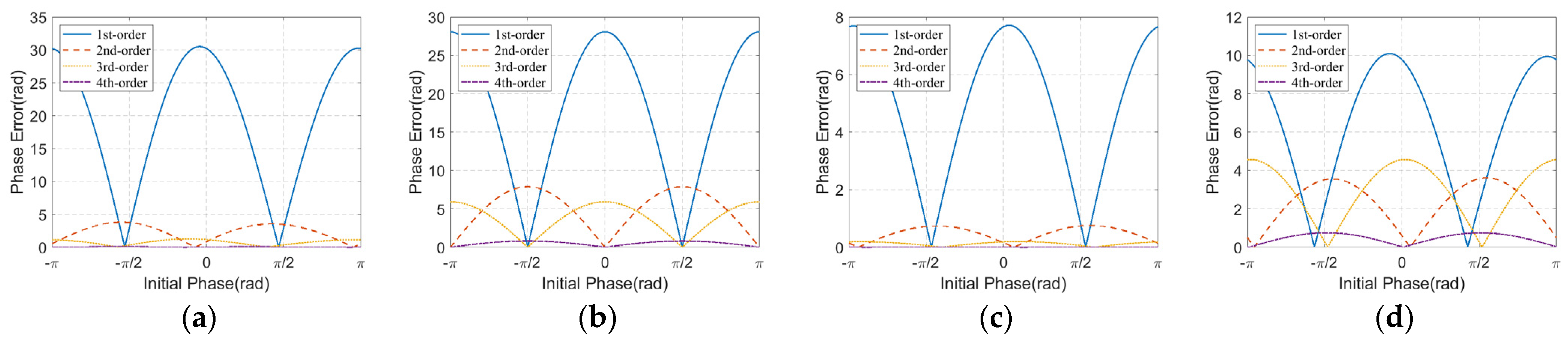
| Phase Error Order | Effects on SAR Azimuth Images |
|---|---|
| 1 | Peak displacement |
| 2 | Defocus of impulse response, decrease of peak amplitude |
| 3 | Unbalanced sidelobes, peak displacement, and amplitude decrease |
| 4 | Symmetrical increase of sidelobe, decrease of peak amplitude |
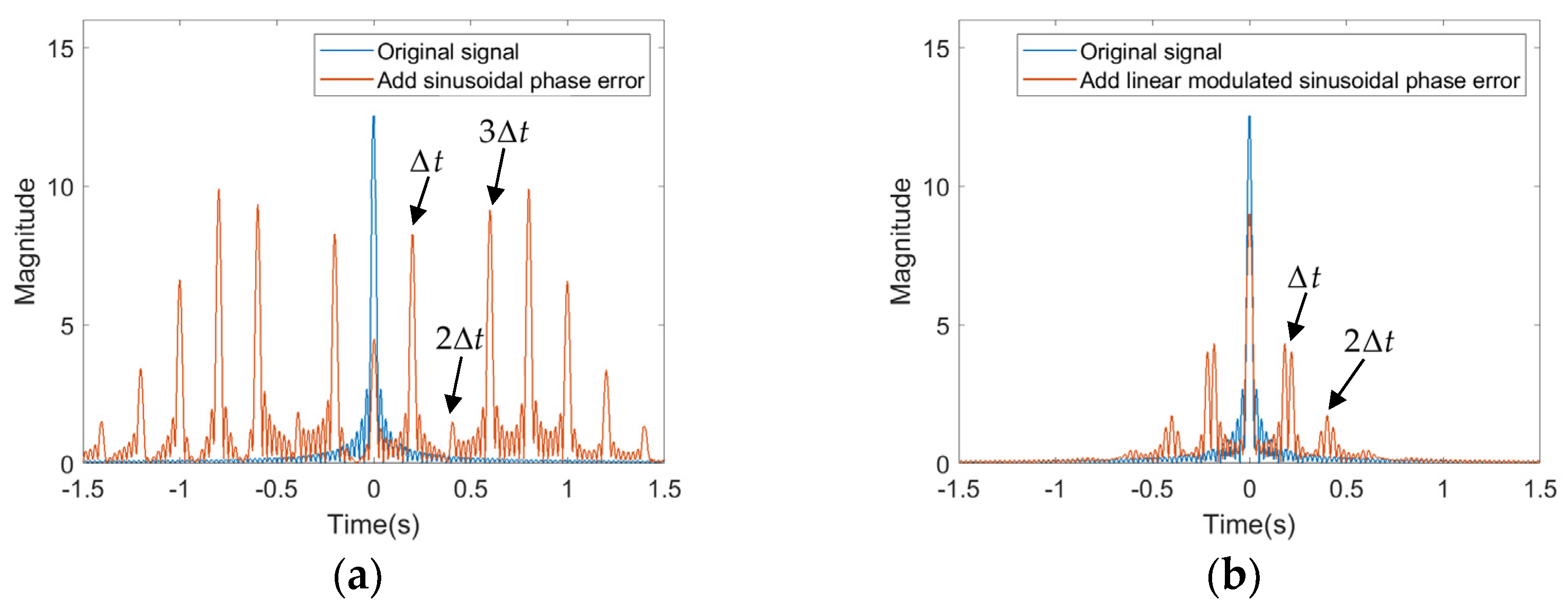
| Higher-order | Paired echoes, ghost images |
| Data | Center Position | Parameter | Value |
|---|---|---|---|
| 28-12-2019 08:14 (local time) | 37°39.815N 121°29.812E | Wind speed | 4.8 m/s |
| Wind direction | 211.2° | ||
| Wave height | 0.7 m | ||
| 28-12-2019 14:14 (local time) | 37°40.395N 121°31.293E | Wind speed | 4.0 m/s |
| Wind direction | 209.0° | ||
| Wave height | 0.5 m |
| Ship State | Variation Range (deg) | Standard Deviation (deg) | ||||
|---|---|---|---|---|---|---|
| Roll | Pitch | Yaw | Roll | Pitch | Yaw | |
| Unanchored | 7.14 | 3.66 | 14.59 | 1.23 | 0.49 | 4.84 |
| Anchored | 6.30 | 2.63 | 5.71 | 1.22 | 0.45 | 1.64 |
| Navigating | 6.53 | 2.71 | 33.39 | 0.99 | 0.48 | 9.36 |
Publisher’s Note: MDPI stays neutral with regard to jurisdictional claims in published maps and institutional affiliations. |
© 2021 by the authors. Licensee MDPI, Basel, Switzerland. This article is an open access article distributed under the terms and conditions of the Creative Commons Attribution (CC BY) license (https://creativecommons.org/licenses/by/4.0/).
Share and Cite
Zhou, B.; Qi, X.; Zhang, J.; Zhang, H. Effect of 6-DOF Oscillation of Ship Target on SAR Imaging. Remote Sens. 2021, 13, 1821. https://doi.org/10.3390/rs13091821
Zhou B, Qi X, Zhang J, Zhang H. Effect of 6-DOF Oscillation of Ship Target on SAR Imaging. Remote Sensing. 2021; 13(9):1821. https://doi.org/10.3390/rs13091821
Chicago/Turabian StyleZhou, Binbin, Xiangyang Qi, Jiahuan Zhang, and Heng Zhang. 2021. "Effect of 6-DOF Oscillation of Ship Target on SAR Imaging" Remote Sensing 13, no. 9: 1821. https://doi.org/10.3390/rs13091821
APA StyleZhou, B., Qi, X., Zhang, J., & Zhang, H. (2021). Effect of 6-DOF Oscillation of Ship Target on SAR Imaging. Remote Sensing, 13(9), 1821. https://doi.org/10.3390/rs13091821