RSIMS: Large-Scale Heterogeneous Remote Sensing Images Management System

Abstract

With the remarkable development and progress of earth-observation techniques, remote sensing data keep growing rapidly and their volume has reached exabyte scale. However, it’s still a big challenge to manage and process such huge amounts of remote sensing data with complex and diverse structures. This paper designs and realizes a distributed storage system for large-scale remote sensing data storage, access, and retrieval, called RSIMS (remote sensing images management system), which is composed of three sub-modules: RSIAPI, RSIMeta, RSIData. Structured text metadata of different remote sensing images are all stored in RSIMeta based on a set of uniform models, and then indexed by the distributed multi-level Hilbert grids for high spatiotemporal retrieval performance. Unstructured binary image files are stored in RSIData, which provides large scalable storage capacity and efficient GDAL (Geospatial Data Abstraction Library) compatible I/O interfaces. Popular GIS software and tools (e.g., QGIS, ArcGIS, rasterio) can access data stored in RSIData directly. RSIAPI provides users a set of uniform interfaces for data access and retrieval, hiding the complex inner structures of RSIMS. The test results show that RSIMS can store and manage large amounts of remote sensing images from various sources with high and stable performance, and is easy to deploy and use.

1. Introduction

Since the first photograph of Earth was captured from outer space by German V2 rocket on 24 October 1946 [1], hundreds of earth observation satellites have been launched and volumes of remote sensing data keep growing explosively. According to the definition of Gartner, remote sensing data have become a new kind of typical big data with three typical features, namely high-volume, high-velocity, and high-variety [2].

From the aspect of high-volume and high-velocity, lots of institutions have archived petabyte-scale of remote sensing data and kept growing rapidly. For example, DigitalGlobe has accumulated more than 90PB remote sensing imagery back to 1999 and increases by 70TB per day [3]. The volume of remote sensing data in ECMWF (European Centre for Medium-Range Weather Forecasts) has reached 100PB with an annual growth rate of about 45% [4]. From 2007 to 2018, the volume of remote sensing data archived in CCRSDA (China Center for Resources Satellite Data and Application) has increased from 0.18PB to 35PB [5].

In terms of high-variety, we can see that remote sensing data from different satellites have many differences, such as spatial range, spectral range, pixel resolution, revisit period, etc. Moreover, different images from different sources are stored with different structures [6]. Due to these differences, lots of remote sensing data from different sources are stored independently, just like isolated data islands, making it hard to make full usage of these data.

Besides the above three features, “high-value” is another feature of big remote sensing data: rich information contained in remote sensing data can’t only help us learn about the Earth more comprehensively, but also play a very import role in environment protection, natural hazard forecast, agricultural development, etc. [7,8,9].

Faced with these challenges of big remote sensing data, the traditional way that process data with standalone software on ordinary PC is impractical. Even on HPC with high performance and large capacity, there exist many limitations on data sharing, capacity scalability, etc. Nowadays, the distributed storage system has been proved instrumental in the effort to dealing with big remote sensing data storage and access.

Distributed storage system can integrate multiple commodity physical servers into a virtual single high-capacity server from the user’s point of view. Compared with traditional standalone storage systems, distributed storage system can provide large and scalable storage space, and is very easy and efficient for data sharing and access. Moreover, unlike a normal standalone filesystem, it can also provide security mechanisms to prevent unauthorized data access or unexpected data corruption caused by server failures.

Popular free and open-source distributed data storage systems include Lustre(2003) [10], HDFS(2005) [11], GlusterFS(2005) [12], MooseFS(2008) [13], CEPH(2010) [14], Alluxio (2013) [15], SeaweedFS(2015) [16], etc. Lots of researchers have tried to manage remote sensing data in the above storage systems. Ma et al. adopted Lustre in the dynamic DAG task scheduling for remote sensing data parallel process [17]. Kou et al. explored remote sensing image processing methods based on HDFS [18], and similar work include [19,20]. MooseFS is used by gscloud (one of the most popular remote sensing data providers in China) to store various kinds of remote sensing data.

Besides the above open-source distributed storage systems, Google Earth Engine took Colossus, the successor to the Google File System, as the remote sensing data storage system [21]. NASA has migrated Landsat 8 images to AWS distributed object storage system, which can be accessed via Amazon S3 [22].

Although these popular distributed storage systems can provide large scalable capacity and high I/O performance, there are some limitations for these storage systems to manage large-scale remote sensing images because they just regard remote sensing images as big unstructured binary files, ignoring their specific data structures and spatiotemporal features. HDFS, for example, was designed and optimized for large file (gigabytes to terabytes in size) batch processing. Internally, files are split into one or more data blocks of a pre-determined size (default 128 MB). However, lots of remote sensing image band files are less than 200 MB, e.g., Landsat 8 image band files are about 100 MB. Indeed, HDFS put more emphasis on high throughput rather than low latency, which is not suitable for real-time interactive data analysis. Moreover, HDFS expects that data process programs should run on the node where the data were located, which increases the burden of data nodes and limits the program development and deployment. HDFS follows a master-slave architecture, where all the metadata (data blocks locations, data nodes information, etc.) are stored in the master node (NameNode). The architecture has SPOFs (single point of failure) and limits the expansion of storage space.

Besides the system architecture and internal storage structure, most of above systems provide different distinct interfaces, which requires rewriting the related programs if remote sensing data are migrated into these storage systems.

Considering the specific features of remote sensing data and limitations of current storage systems, we proposed the remote sensing images management system (RSIMS), a new distributed storage system for large-scale remote sensing data storage, access and retrieval. In addition to excellent data compatibility and capacity scalability, RSIMS provides efficient spatiotemporal retrieval interfaces based on the distributed spatial index, which is built with global multi-level Hilbert grids. Test results with 14,187,101 remote sensing images show that RSIMS can retrieve millions of remote sensing images intersected with a very large geospatial region within less than 10 seconds. Besides metadata management, RSIMS provides two GDAL-compatible interfaces, which allows popular tools and software access the remote sensing image files in RSIMS directly.

RSIMS is designed for remote sensing data owners to provide data access and retrieval service for authorized users. From the perspective of users, RSIMS is a storage software deployed on multiple remote servers. Large amounts of remote sensing data are uploaded into RSIMS by administrators and then accessed by common users remotely.

The remainder of this paper is structured as follows. Section 2 describes RSIMS in detail, including the system architecture, the data structures and easy-to-use interfaces design. Section 3 evaluates the performance of RSIMS. Section 4 discusses the results of test. Section 5 makes a summary about the main work of this paper and the performance of RSIMS.

2. Materials and Methods

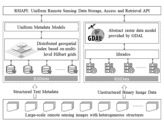
2.1. The System Architecture of RSIMS

As illustrated in Figure 1, RSIMS adopts a modular and layered architecture. The top layer is RSIAPI which hides the complex and diverse inner storage schemas and provides users a set of uniform interfaces for remote sensing images storage, access and retrieval. The bottom layer is divided into two relatively independent modules: RSIMeta and RSIData. RSIMeta, as shown in the right part of Figure 1, employs the reliable and efficient PostgreSQL database cluster to store the structured metadata of remote sensing images and then index these images with the distributed spatial index built based on multi-level Hilbert grids. RSIData, as shown in the left part of Figure 1, stores the remote sensing image files in the form of objects in CEPH, which is a distributed object storage system with high I/O performance and good capacity scalability, and then provides users two types of GDAL compatible I/O interfaces.

The following content will be divided further into three parts to introduce RSIMS. The first part introduces the details of distributed spatial index building and multi-source heterogeneous remote sensing images integration which are key to the performance of RSIMS. The second part introduces the details of remote sensing image files storage and GDAL compatible interfaces design. The last part introduces the usage of RSIAPI.

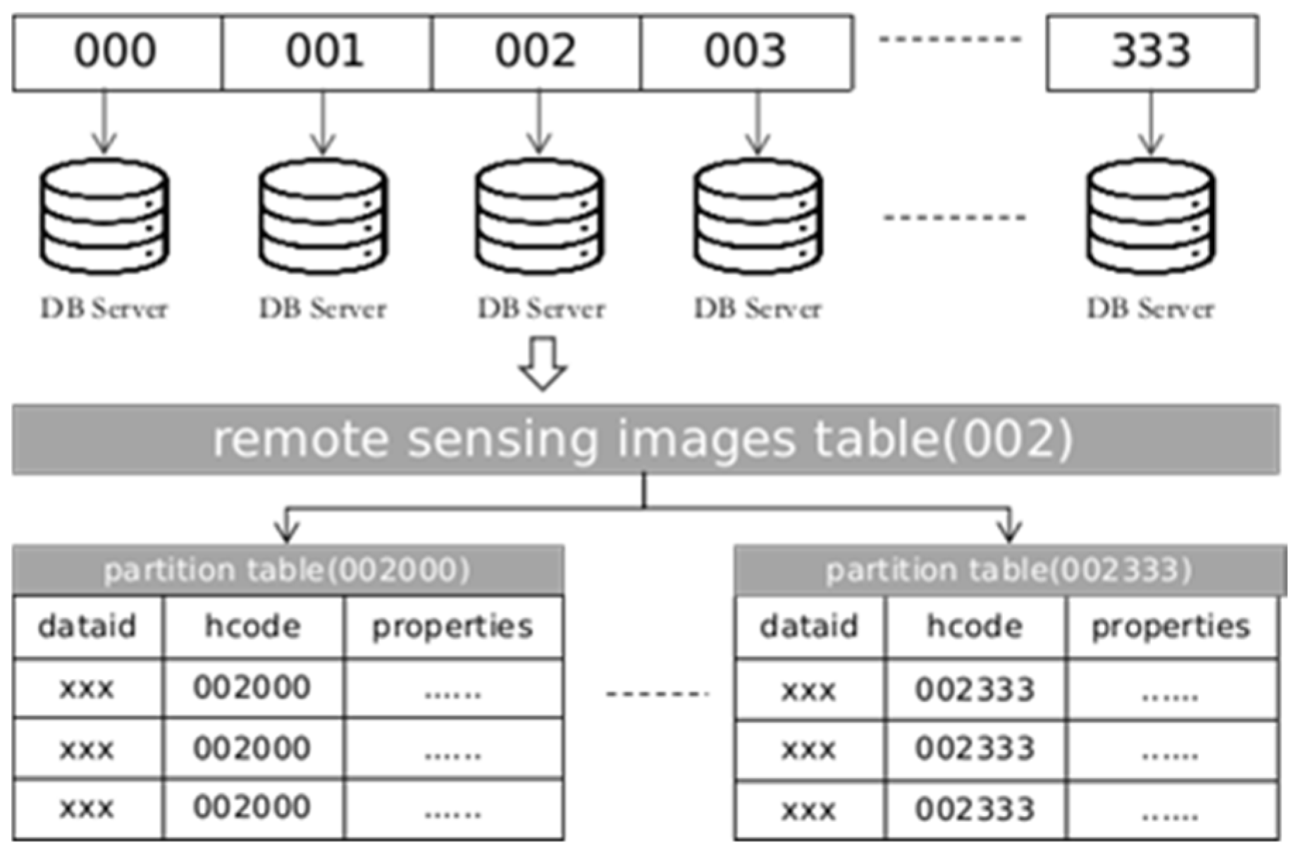
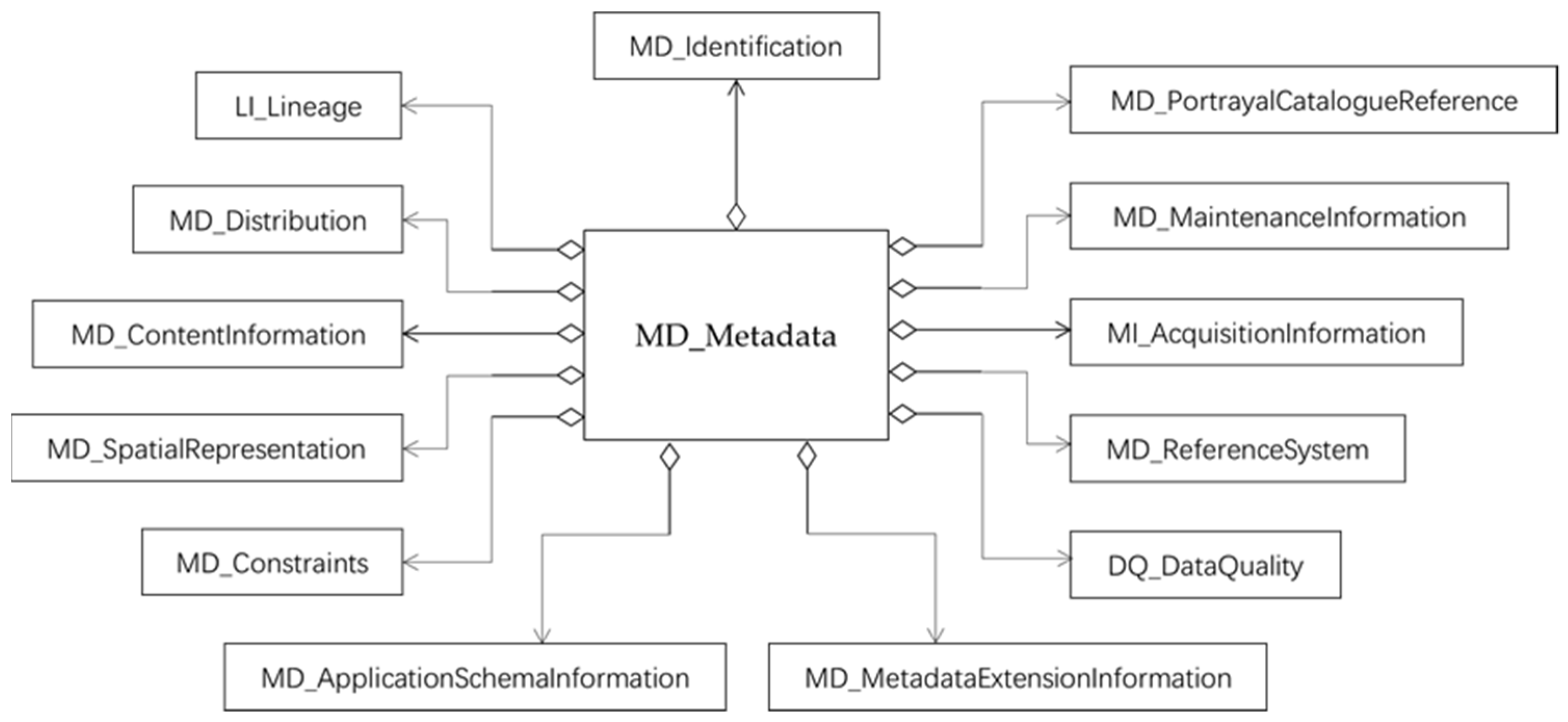
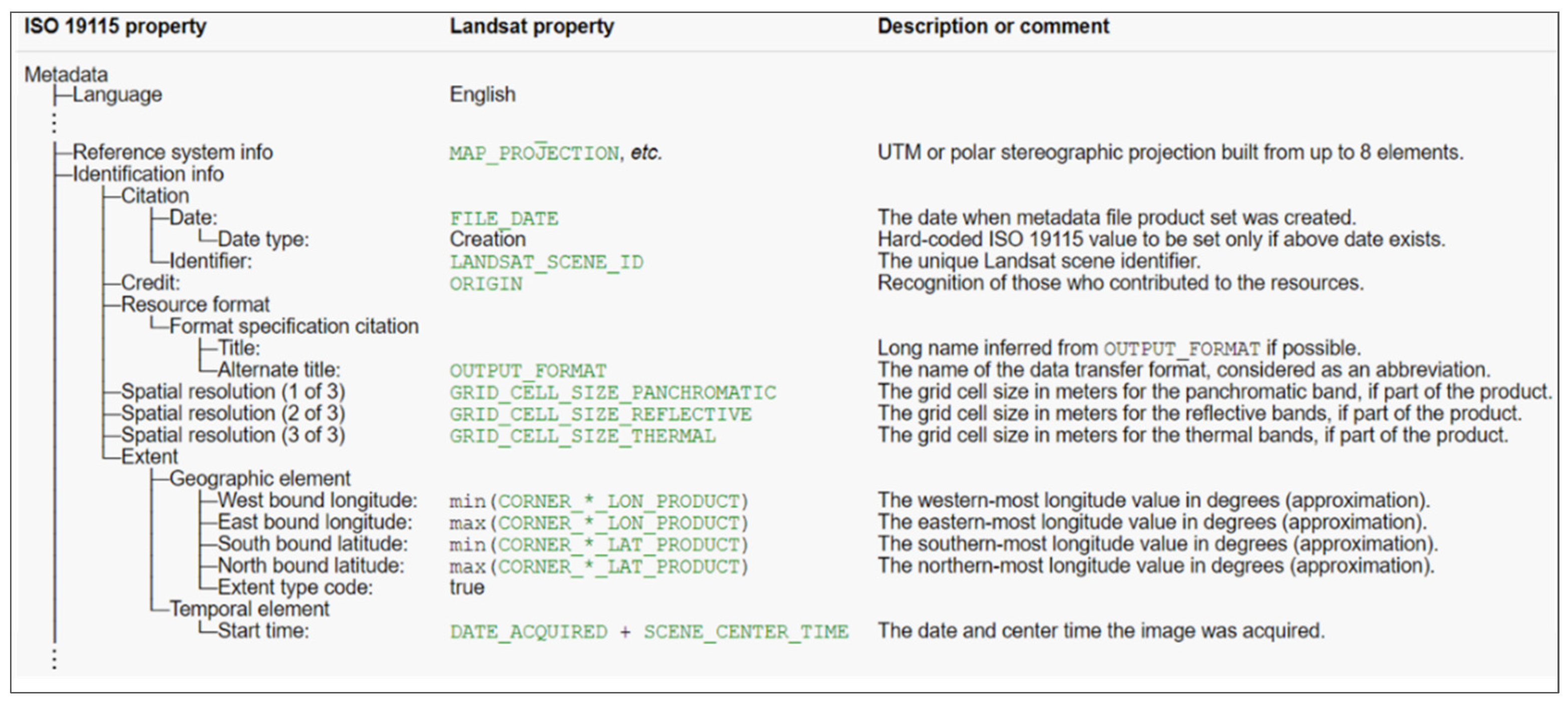
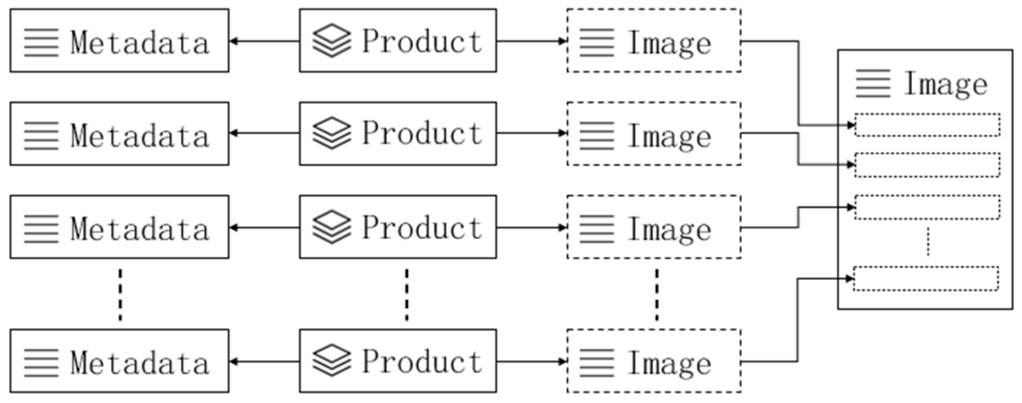
2.2. RSIMeta: Metadata Management of Large-Scale Images with Heterogeneous Structures

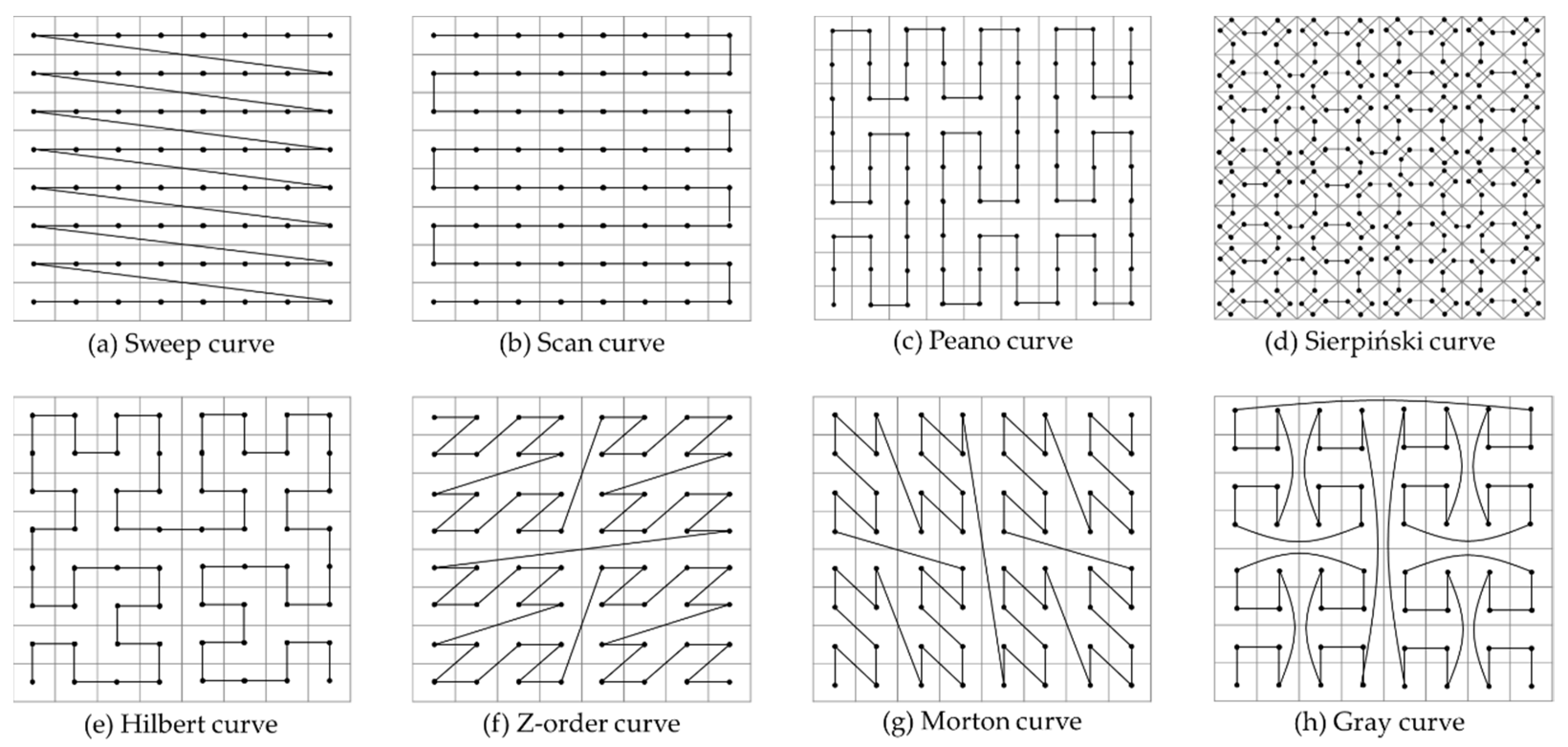
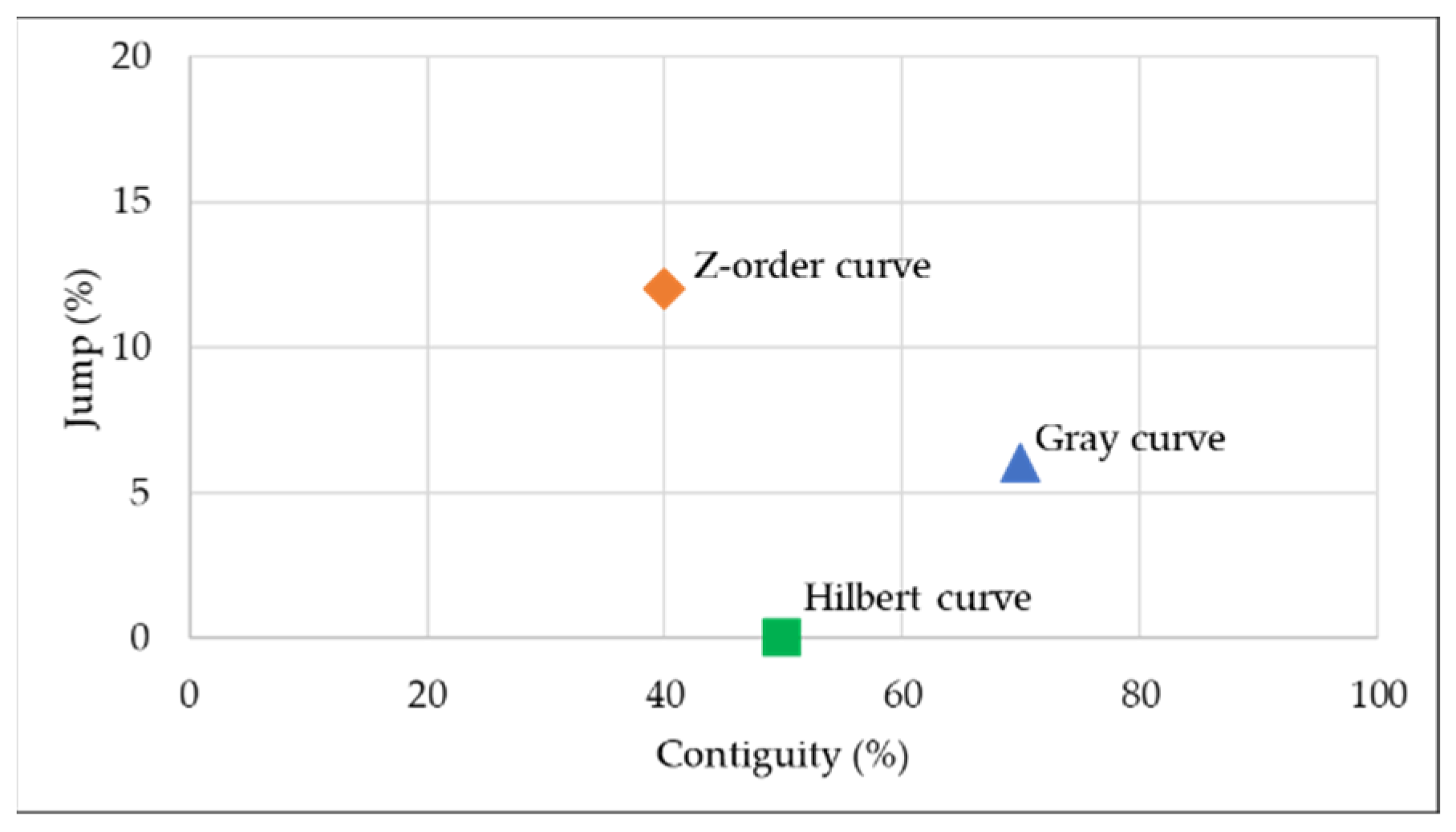
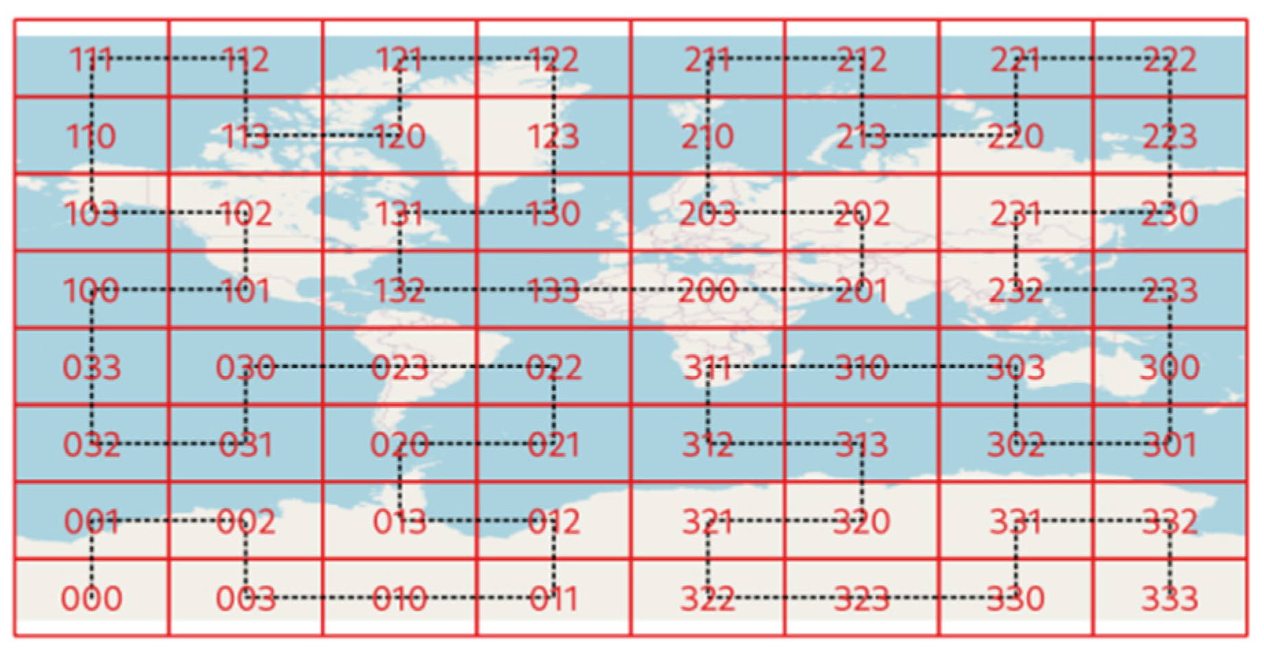
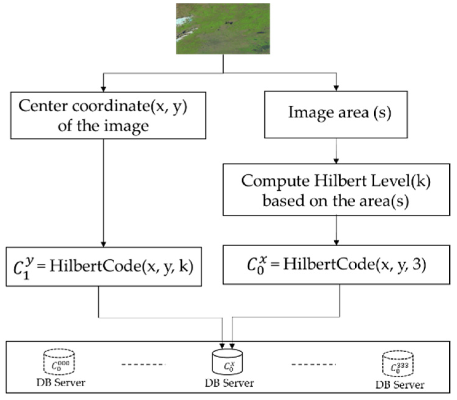
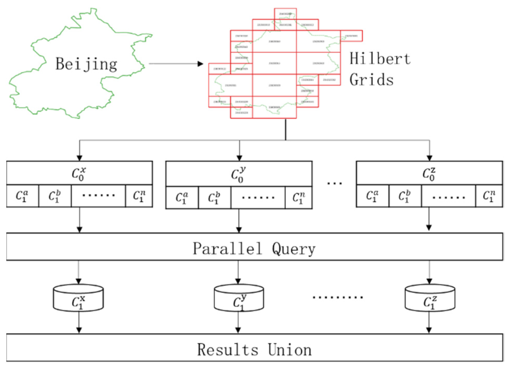
2.2.1. Distributed Spatial Index Based on Multi-Level Hilbert Grids

One of the most significant differences between remote sensing data and other types of common data is its complex and diverse attributes, such as date acquired, spatial location, pixel size, cloud coverage, etc. Attributes other than spatial location are all stored with the basic data types, such as integer, string, datetime, etc. Data retrieval based on these normal attributes have been optimized very well. However, geospatial query based on polygonal region is still relatively slow due to the high time complexity, which is a bottleneck for efficient remote sensing images retrieval.

Building spatial index is an efficient way to improve the retrieval performance. Traditional spatial index, e.g., R-Tree [23], is inappropriate for geospatial query with irregular-shaped polygon regions in the distributed storage systems. To support efficient geospatial query of large amounts of remote sensing images stored in RDMS cluster, the paper designed a distributed spatial index based on the space-filling curve.

Space-filling curve (SFC) gives a way of linear mapping from multi-dimensional space to one-dimensional space, which makes it possible to apply the optimized techniques designed for one-dimensional space to multi-dimensional space. Compared to the traditional spatial index, SFC provides a simpler but more effective way to index large amounts of geographical objects stored in distributed storage systems. Since Giuseppe Peano described the first SFC in 1890 [24], numerous kinds of SFCs with different shapes have been discovered. SFCs have been widely used by lots of applications for better performance, such as multi-attribute hashing [25,26,27], task scheduling [28,29], image compression [30], and file storage [31]. Figure 2 shows eight typical SFCs.

The major difference of these SFCs is the order they traverse these points in the multi-dimensional space. Different traversal orders determine how a SFC can preserve the locality of points from the multi-dimensional space in the mapped one-dimensional space, which is a key criterion to measure the quality of an SFC.

Sweep curve and scan curve just preserve the locality in a single direction, but in the other direction, the distance of adjacent points is very long and would increase as the data volume grow. Remote sensing images are usually retrieved based on spatial planar regions, which requires that locality of two directions should be preserved as much as possible. So, sweep curve and scan curve are not appropriate for remote sensing images organization and retrieval.

The Peano curve is similar to the Hilbert curve. The Hilbert curve is designed based on the same idea as the Peano curve [32]. The difference between them is that the Peano curve is constructed recursively by subdividing the square into nine smaller squares, while the Hilbert curve is constructed recursively by subdividing the square into four smaller squares. For most GIS applications (e.g., TMS protocol, image pyramids used in GEE), the latter way is more efficient and easier to use.

Unlike other SFCs, Sierpiński curve [33] is constructed based on isosceles right triangles instead of squares and has excellent symmetrical property, which has been used in TSP [34], parallel computing [35], etc. However, almost all the remote sensing images are generated and organized based on squares instead of triangles, so the Sierpiński curve is also not appropriate to index remote sensing images.

After filtering out the sweep curve, scan curve, Peano curve, and Sierpiński curve based on the unique requirements of remote sensing applications, there are four candidate SFCs. Z-order curve and Morton curve are identical other than direction, and the difference can be ignored for remote sensing images geospatial metadata. So, we would further compare Hilbert curve, Z-order curve and Gray curve to select the optimal SFC for large amounts of remote sensing images indexing.

To quantify the locality-preserving property of a SFC, Mohamed Mokbel [36] proposed a description vector composed of the percentages of five segment types: jump, contiguity, reverse, forward, and still. If the distance of two points connected by a segment in SFC is equal to one in the origin multi-dimensional space, the segment connecting the points is a contiguity segment. Otherwise, if the distance is greater than one, it is a jump segment; If the distance is equal to zero, it is a still segment. If the direction from a point to another point doesn’t change after mapped, the segment connecting the points is a forward segment, otherwise it’s a reverse segment. Based on the above definition, jump and contiguity are the key factors for geospatial query performance of remote sensing images. The other three factors are important for applications dependent on the data access order. The jump and contiguity percentage comparisons of the Hilbert curve, Gray curve, and Z-order curve are shown as Figure 3.

From Figure 3, we can find that the Hilbert curve and Gray curve are better than Z-order curve due to the lower jump and higher contiguity. Besides the above methods, Bongki Moon et al. [37] measured the locality-preserving property with the number of clusters required by a query region of any arbitrary shape. With closed-form formulas and experiments, Hilbert curve was proven to be superior with better clustering; To compare Scan curve, Z-order curve, Gray curve and Hilbert curve, H V Jagadzsh [38] constructed several test cases to evaluate the performance of file blocks fetching with different SFCs, and the final results showed that Hilbert curve outperformed other SFCs in all the test cases.

Based on the above comparative analysis, Hilbert curve was adopted by RSIMeta due to its better locality-preserving property and recursive structure of multi-level squares. Based on Hilbert curve, we designed a distributed spatial index for remote sensing metadata storage and retrieval, which can be used to select quickly images intersected with a very large geographical area from billions of remote sensing images.

2.2.2. Remote Sensing Images Index and Retrieval Based on Hilbert Curve

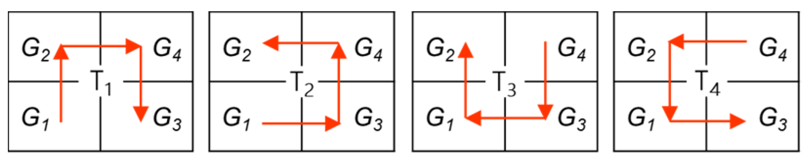
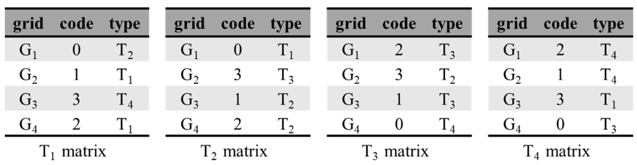
Based on Hilbert curve, we first divide the global world (−180, −90, 180, 90) into multi-level grids from 0 to 32. The level 0 grid is the biggest grid covering the whole world. The size of the grid in Level k is $\left(360/2^k , 180/2^k \right)$. To distribute remote sensing images across different database servers, we adopt the level 3 Hilbert grids as the basic reference grid system, shown as Figure 4. All the remote sensing images intersecting with the same Hilbert grid are stored in the same database.

The black dotted line in Figure 4. is the path along which the Hilbert curve connect all the grids. These grids are encoded from 000 to 333 expressed with quaternary system, and all the remote sensing images are encoded with the level 3 Hilbert codes (denoted by $C_0$) based on their center coordinates. Remote sensing images encoded with different codes can be stored in different databases which would improve the capacity scalability and I/O concurrency.

The amount of remote sensing images in a single grid may still be too large. For better retrieval efficiency, the remote sensing image in a single grid is further encoded into a longer Hilbert code (denoted by $C_1$). After that, complex spatial intersection operation can be transformed into simple string code matching. The structure of two-tier distributed spatial index is shown as Figure 5.

The cost of Hilbert code computation is key to the efficiency of distributed spatial index building. To speed up the process, we implemented the Hilbert code calculating algorithm based on the state-transition matrix, which is described in detail below.

As shown in Figure 6, Hilbert curve have four types of basic shapes, which are encoded respectively as $T_1$, $T_2$, $T_3$, $T_4$. All Hilbert curves are constructed from these four basic shapes recursively. To describe the construction rules clearly, we encode the sub-grids respectively as $G_1$,$G_2$,$G_3$,$G_4$ based on their related locations.

Suppose that $T_p$ is the type of Hilbert curve that connecting four grids ($g_k^1$, $g_k^2$, $g_k^3$, $g_k^4$) in $leve{l}_k$, and $T_c$ is the type of Hilbert curve connecting four grids ($Grid{s}_{k-1}$) in $leve{l}_{k-1}$ which are generated by subdividing one of the above four grids. The rules of Hilbert curve construction are listed as below:

• $T_c$ is same as $T_p$ if $Grid{s}_{k-1}$ are generate from $g_k^2$ or $g_k^4$;
• $T_c$ is generated from rotating $T_p$ 90 degrees clockwise if $Grid{s}_{k-1}$ are generate from $g_k^1$;
• $T_c$ is generated from rotating $T_p$ 90 degrees counterclockwise if $Grid{s}_{k-1}$ are generate from $g_k^3$;

Based on the above rules, we can get the following curve-transition matrixes, shown as Figure 7. By looking up these matrixes directly, the time complexity of calculating the Hilbert code of sub-grid is O(1).

Based on the matrixes, Hilbert code computing algorithm is described as the following pseudo codes. The Hilbert code of a grid is computed recursively from higher level to lower level. Because the time complexity of every step is O(1), the total time complexity of Algorithm 1 is O(n).

Algorithm 1 Hilbert code computing

function HilbertCode(x, y, k){ ””” params: x: the longitude value of a point, −180 ≤ x ≤ 180 y: the latitude value of a point, −90 ≤ y ≤ 90 k: the level of Hilbert grids, 0 ≤ k ≤ 32 ””” hcode, htype = 0, T1 while k > 0:   m, n = HilbertGrid(k, x, y)   mb, nb = binary(m), binary(n)   mk, nk = mb & (2 ≪ k), nb & (2 ≪ k)   grid_idx= mk*2 + nk   ck = query_code(M[htype], grid_idx)   hcode = hcode ≪ 2 | ck   htype = query_type(M[htype], grid_idx)   k = k – 1 return hcode }

Auxiliary variables and functions are explained as follows:

• M = [T1 matrix, T2 matrix, T3 matrix, T4 matrix];
• function HilbertGrid(k, x, y): calculate the position of the grid in Cartesian coordinate system;
• function binary(m): convert decimal to binary;
• function query_code(matrix, grid): query the code from the curve-transition matrix of some type based on the identification of the grid;
• function query_type(matrix, grid): query the Hilbert curve shape type of level(k − 1) from the curve-transition matrix of some type based on the identification of the grid.

Considering that remote sensing images from different sources have different sizes, the second level (the param(k) in Algorithm 1) should be determined dynamically. The rule is that the expected Hilbert level should be the smallest one whose corresponding grids is larger than the average size of all remote sensing images from the same platform. Taking the Landsat for example, the average area of all Landsat images is about 4 × 104 km², so the second Hilbert level for Landsat images is 5.

The whole process can be illustrated with Figure 8. Remote sensing images of the same type are encoded into Hilbert codes ($C_0$) based on the basic 8*8 global grids for distributed storage, and then for optimized spatial intersection query, every single remote sensing image is further encoded into a longer Hilbert code ($C_1$), which is dynamically based on the image size.

To take advantage of the multi-level Hilbert grids storage structure, the spatial query region is also subdivided into multiple Hilbert grids for better retrieval performance. Finding a Hilbert grid which just contains the query area is simple and can reduce the query scope, but this way would include too many disjoint images, which still need lots of time to select the target images.

We designed another algorithm to subdivide the query area into Hilbert grids which are consistent with remote sensing datasets. After that, complex and slow spatial intersection computing can be transformed to simpler and faster string matching. The process includes two parts: one for calculating Hilbert grids coverage, and the other for Hilbert grids encoding. The steps of calculating Hilbert grids coverage are described as follows.

Suppose that S is the vector boundary of the remote sensing image, B is the bounding box of S, and G is the minimum set of grids covering B. The relationship of S (blue line zone), B (green line zone), and G (red line zone) is shown as Figure 9.

The steps are described as follows:

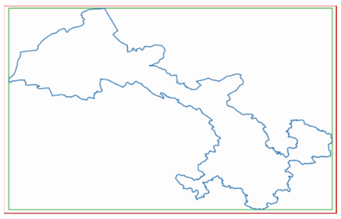
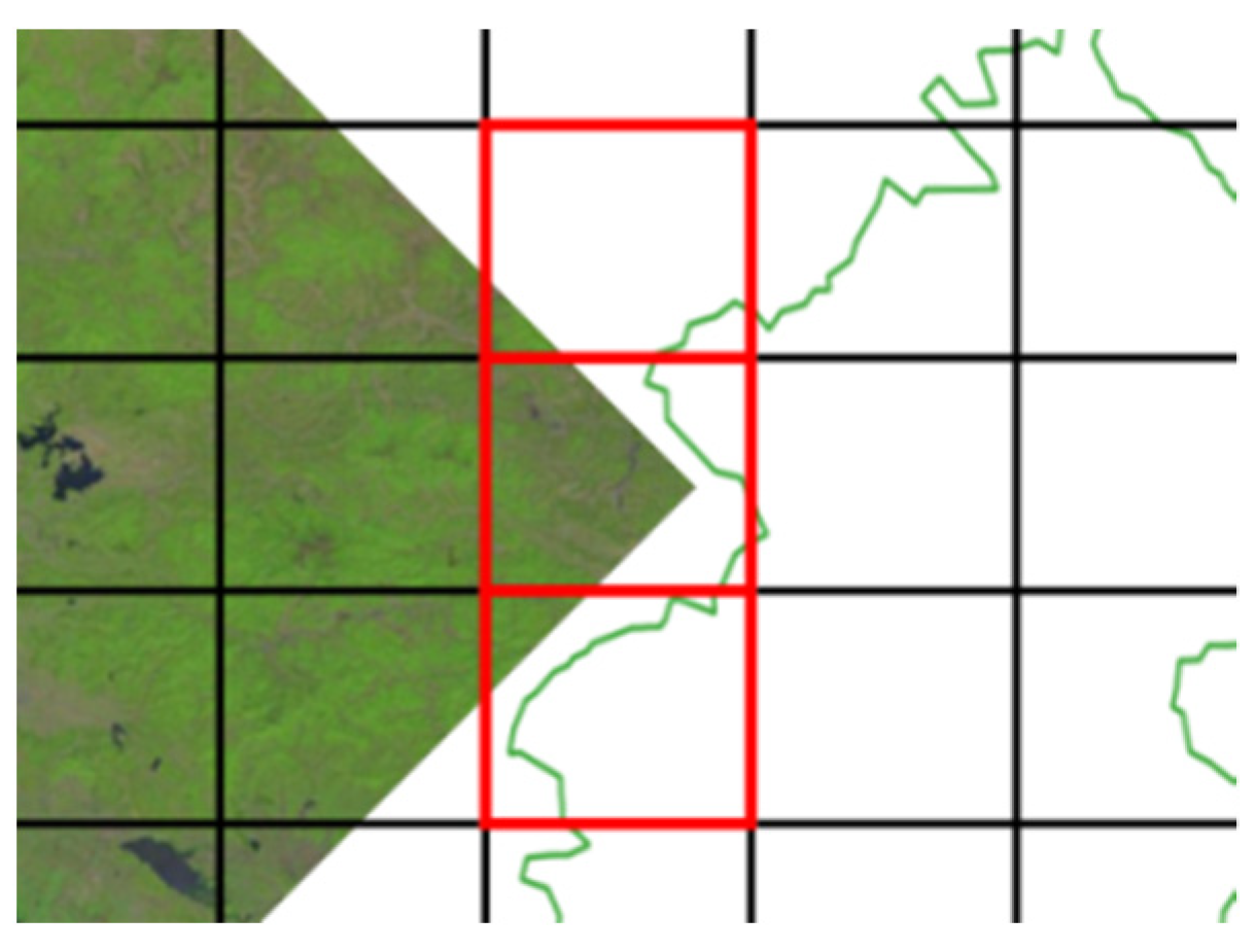
• Subdivide G into four sub-regions (represented by SG) of almost the same size;
• Iterate over SG, and evaluate the spatial relationship between each sub-region of SG and S. If the sub-region is contained in S, then put the sub-region in the list of results; if the sub-region intersects with S, then set the sub-region as a new G, and then return to step (1); if the sub-region and S are disjoint, then omit the sub-region.

Pseudo codes are show as Algorithm 2:

Algorithm 2 Hilbert grid coverage

GridRegions = [ ] function HilbertCoverage(region) { ext = GridExtent(region) if ext < GRID_EXT * 4:   GridRegions.push(ext)   return rgs = QuarterDivide(region) for rg in rgs:   if S.contains(rg):     GridRegions.push(rg)   if S.intersects(rg):     HilbertGrids(rg)

After processed by Algorithm 2, regions generated still can’t be used directly because some regions are not consecutive in the Hilbert code order and some smaller regions can be merged into a bigger one for better retrieval performance.

As shown in Figure 10, green grids are consistent with Hilbert multi-level grids and blue grids generate from Algorithm 2. From Figure 10, we can know that some blue grids can’t be encoded by Hilbert curve, so we design Algorithm 3 to subdivide-and-merge blue grids into green grids. Steps of divide-and-merge Hilbert girds are described as below:

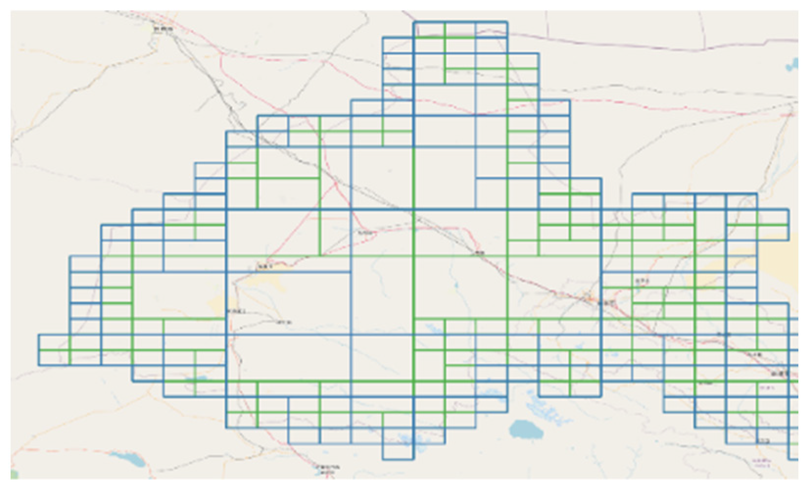
• Divide all the sub-regions into basic Hilbert grids and encode these grids.
• Sort these Hilbert codes into an ordered list and then split the list into successive segments.
• Iterate over these segments, and merge grids of each segment into a bigger Hilbert grid.

Note that only four adjacent grids connected by a basic Hilbert curve (one of Figure 6) can be merged. The process can be illustrated by Figure 11.

Pseudo codes are show as Algorithm 3:

Algorithm 3 Hilbert grid split-and-merge

LEVEL = k function HilbertGrids(regions) { hcodes = [ ] for reg in regions:   grids = HilbertSplit(reg)   for grid in grids:      x, y = GridCenter(grid)     code = HilbertCode(x, y, LEVEL)      hcodes.push(code) segments = HilbertSplit(hcodes) results = [ ] for seg in segments:   codes = HilbertMerge(seg)   results.merge(codes) return results

In summary, the whole process can be illustrated as Figure 12.

As shown in Figure 12, the query region is subdivided first into multi-level Hilbert grids based on the Algorithms 2, and then be sent to different database servers simultaneously for parallel geospatial query. Finally, all the results from the different database servers are collected and merged, and then return to the client.

Note that the purpose of Hilbert grids used in geospatial intersection query is to reduce the number of candidates drastically. Results retrieved with only Hilbert grids are inaccurate, which are illustrated by Figure 13. The green area in the right part of Figure 13 intersects with the red grid but not the left remote sensing image. However, the image covered by the red grids will be regarded as intersection with the green area, which is wrong obviously.

2.2.3. Multi-Source Heterogeneous Remote Sensing Images Integration

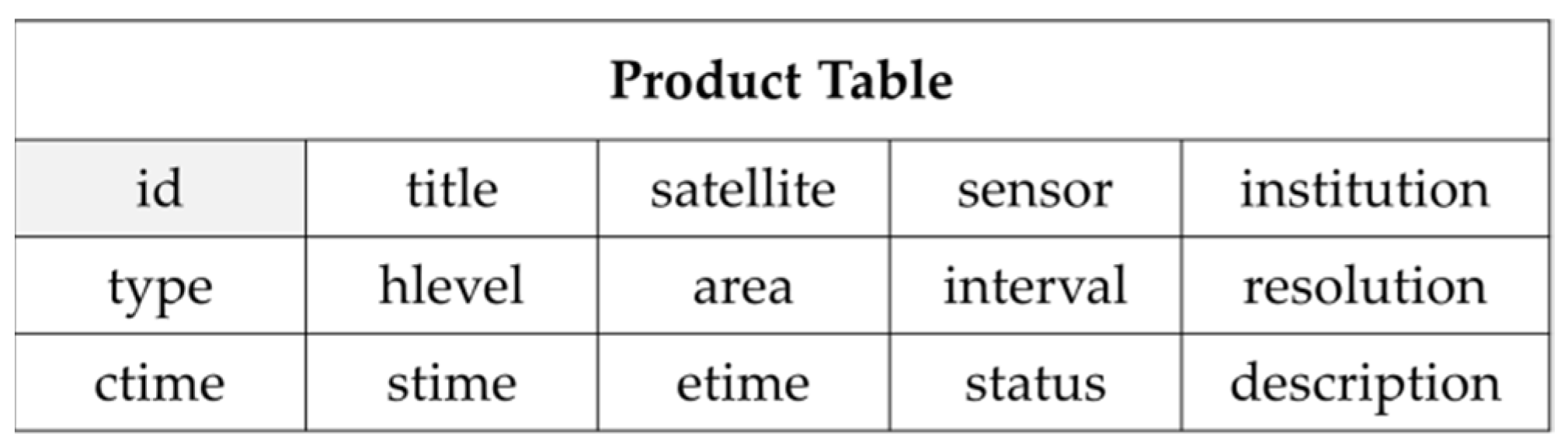
As mentioned in Section 1, challenges of big remote sensing data include not only the large data volumes, but also the wide variety of data structures. In the past decades, hundreds of remote sensing satellites have been launched into spaces. Remote sensing data from these platforms are processed by different organizations and then described with different metadata schemas. Since the early 1990s, lots of national, regional, and international geospatial information metadata standards with different terminologies, structures, and purposes have been developed and applied to different remote sensing products [39,40,41,42]. Ideally, large amounts of remote sensing data from different sources can complement each other to extract more comprehensive and accurate information about the earth. However, incompatible and isolated metadata standards make it hard to take full advantage of all these available data.

Faced with these issues, ISO/TC211, a technical committee of the International Organization for Standardization (ISO), proposed ISO 19115 standard [43] for geospatial metadata in 2003, and then added metadata elements and schemas for imagery and gridded geospatial datasets in the ISO 19115-2 standard [44], which was published in 2009. Now the latest related standard about remote sensing image metadata is “ISO 19115-2, Geographic Information-Metadata-Part 2: Extensions for acquisition and processing” [45] published in 2019, which extends ISO19115-1(2014) and ISO/TS 19115-3(2016). The overall metadata structure of ISO 19115-2 is shown as Figure 14.

ISO 19115 has been widely accepted for geospatial information metadata management and facilitate interoperability of remote sensing data from different sources. Taking Landsat as an example, the mapping from properties of a Landsat image to ISO 19115 metadata is shown as Figure 15.

However, there still exist some different standards which have been adopted by other metadata systems, such as DIF 10, ECHO 10. To support multiple metadata standards continuously, NASA designed Unified Metadata Model (UMM) [46], which provided a cross-walk for mapping between CMR-supported metadata standards based on seven profiles: UMM-C, UMM-G, UMM-S, UMM-var, UMM-Vis, UMM-T, and UMM-Common. These profiles include metadata about datasets, images, end-to-end services, analysis and visualization tools, etc.

Learning from the related experience and concepts of ISO 19115-2 and UMM, we designed a storage schema for remote sensing metadata with different data structures based on the distributed spatial index mentioned above. Just like "Collection" and "Granule" in ISO 19115-2 and UMM, we use "Product" and "Metadata" to store the information of the dataset and image separately. Product is used to store the description information about a dataset whose images are collected from the same source and processed with same methods. Metadata is used to store the detailed properties of the remote sensing image, and Metadata from different products may have different structures. Besides Product and Metadata, we designed another model, Image, which is used to store the common information of the images from different sources. Image is mainly used to improve the performance of large-scale heterogeneous remote sensing images retrieval.

Considering that Product, Image, and Metadata are all structured models, we store their data in the relational database instead of XML files. The overall storage schema of RSIMeta is shown as Figure 16.

In RSIMeta, every Product table has two associated tables: Image and Metadata. Metadata tables of different Products are distinct from each other, but the Image table is shared by all the Products. The distributed spatial index mentioned above is built on the Image table, which supports billions of image items efficient storage and retrieval. The structures of Product table and Image table are shown as Figure 17 and Figure 18 separately.

Some fields of the Product table are self-explained, such as id, title, institution, satellite, sensor, description, etc. Other fields are explained as below:

• “status”: a tag identifying whether the satellite and sensor are still working properly.
• “resolution”: a list including all the distinct resolutions of different bands.
• “type”: the type of the product.
• “hlevel”: the Hilbert level from 0 to 31 which is calculated based on the average image size of the product.
• “interval”: the interval between the time-sequence adjacent images at the same location.
• “area”: the average coverage area of images, whose unit is km².
• “ctime”: the time when the product is created in the table.
• “stime”: the time when the first scene of the product is generated.
• “etime”: the time when the last scene of the product is generated.

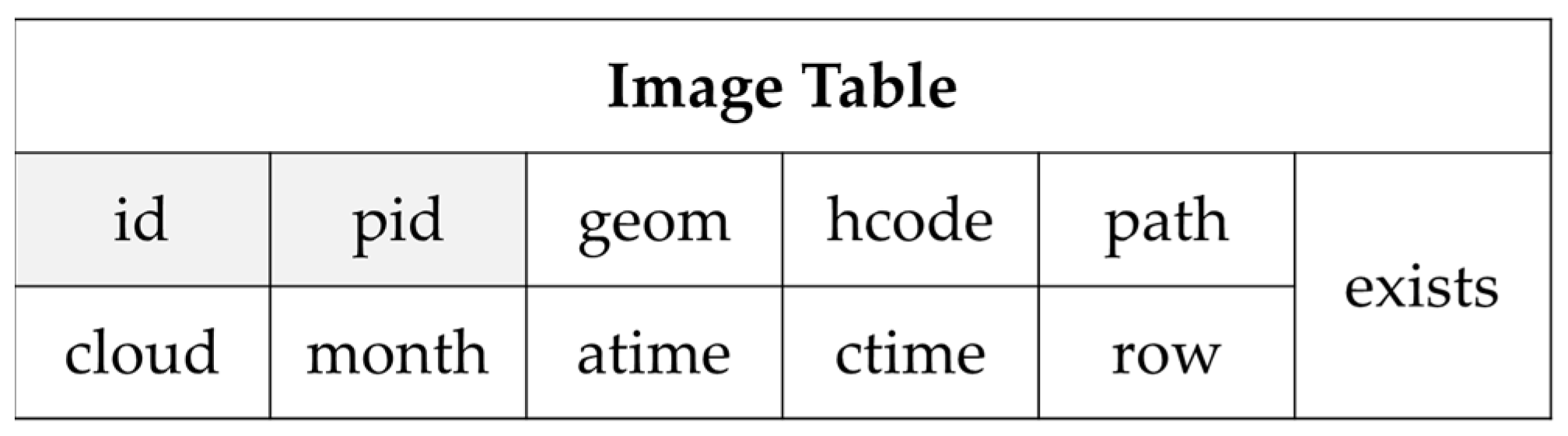
Fields of Image table are explained as below:

• “id”: the unique identification of the image which is defined by the data providers.
• “productid”: identification of the product including the image.
• “hcode”: the code of Hilbert grid calculated based on the image’s center coordinate and the Hilbert level from the corresponding product.
• “geom”: the spatial bounding box of the image whose type is Polygon or MultiPolygon.
• “cloud” is the proportion of the data which is covered by cloud.
• “month” is the month when the data is collected, which can be used to identify season.
• “atime”: the time when the image was acquired.
• “ctime”: the time when the image was stored in the table.

Unlike Image table designed for retrieval, Metadata tables are used to store the detailed information of an image, and Metadata tables of different products have different fields. Therefore, we wouldn’t introduce the detailed fields of different Metadata tables in the paper. The integration flow of remote sensing images from different sources are shown as Figure 19.

The above flow is divided into two steps:

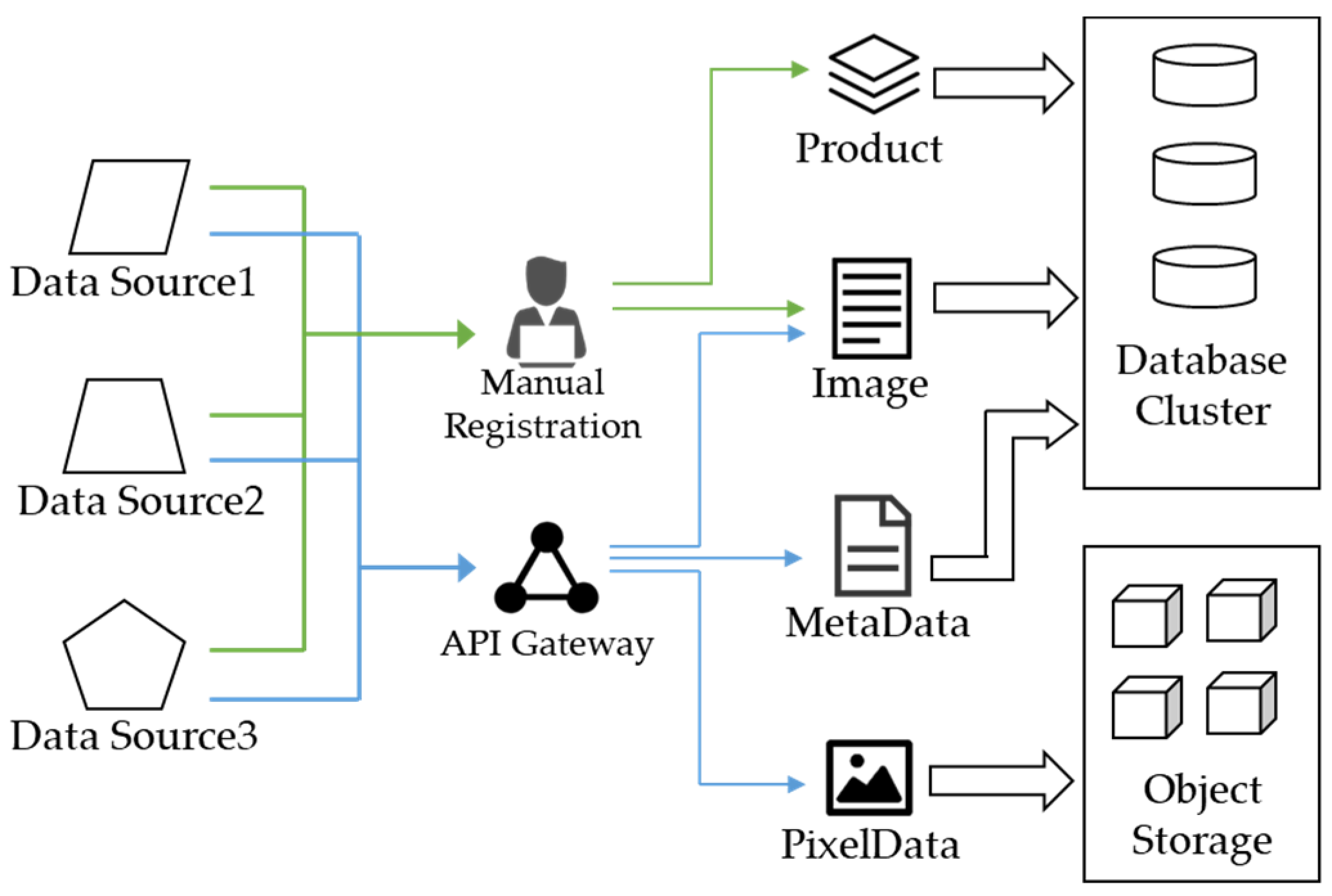
• Manual products registration, described with green lines;
• Data ingestion through API gateway, described with blue lines.

All the work in the first step is performed manually based on professional knowledge and experiences. Attributes and description of some remote sensing images need to be extracted and mapped to fields of the Product and Image table. After that, images of the dataset would be ingested into storage system through the API gateway according to the predefined storage schemas. The binary image files are stored in the distributed object-based storage system, which will be introduced in the next section.

To store remote sensing image metadata in above tables, RSIMeta adopts PostgreSQL to setup the relational database cluster. PostgreSQL is the world’s most advanced open-source relational database, and PostGIS, an open-source spatial extension, enables PostgreSQL to support lots of efficient spatial operations, and have many features rarely found in other spatial databases.

Some comparative studies [47,48] show that PostgreSQL outperforms other popular NOSQL databases in various data retrieval and analysis scenarios. However, this is still a controversial conclusion. To verify the performance of PostgreSQL, we performed some come comparative tests with MongoDB, and the result shows that PostgreSQL is a simpler but more efficient choice for remote sensing images.

Up to now, we have used RSIMS to integrate 180 products with about 100 million of remote sensing images and the number of images keep growing every day.

Table 1. Popular products in RSIMS.

Product	Start Time	Latest Time	Resolutions	Dimensions	HLevel	Size
Landsat 4 MSS	6 August 1982	15 October 1992	80 m	185 km × 185 km	6	341,759
Landsat 4 TM	22 August 1982	18 November 1993	30 m	185 km × 185 km	6	65,870
Landsat 5 MSS	4 March 1984	7 January 2013	80 m	185 km × 185 km	6	1,206,592
Landsat 5 TM	5 March 1984	5 May 2012	30 m	185 km × 185 km	6	4,553,146
Landsat 7 ETM	28 May 1999	30 July 2019	30 m	185 km × 185 km	6	4,281,514
Landsat 8 OLI/TIRS	18 March 2013	30 July 2019	30 m	185 km × 185 km	6	2,554,265
MODIS MCD12Q1 V6	1 January 2001	31 December 2019	500 m	1200 km × 1200 km	4	5983
MODIS MOD09A1 V6	24 February 2000	15 February 2021	500 m	1200 km × 1200 km	4	283,456
MODIS MYD09A1 V6	4 July 2002	2 February 2021	500 m	1200 km × 1200 km	4	251,623
MODIS MYD09GA V6	4 July 2002	24 February 2021	500 m	1200 km × 1200 km	4	2,173,235
MODIS MYD11A1 V6	4 July 2002	16 February 2021	1000 m	1200 km × 1200 km	4	2,142,872
Sentinel-1 SAR GRD	3 October 2014	24 February 2021	10 m	400 km × 400 km	5	41,915
Sentinel-2A MSI	28 March 2017	24 February 2021	10 m 20 m 30 m	290 km × 290 km	6	9,064,645

shows part of remote sensing products in RSIMS.

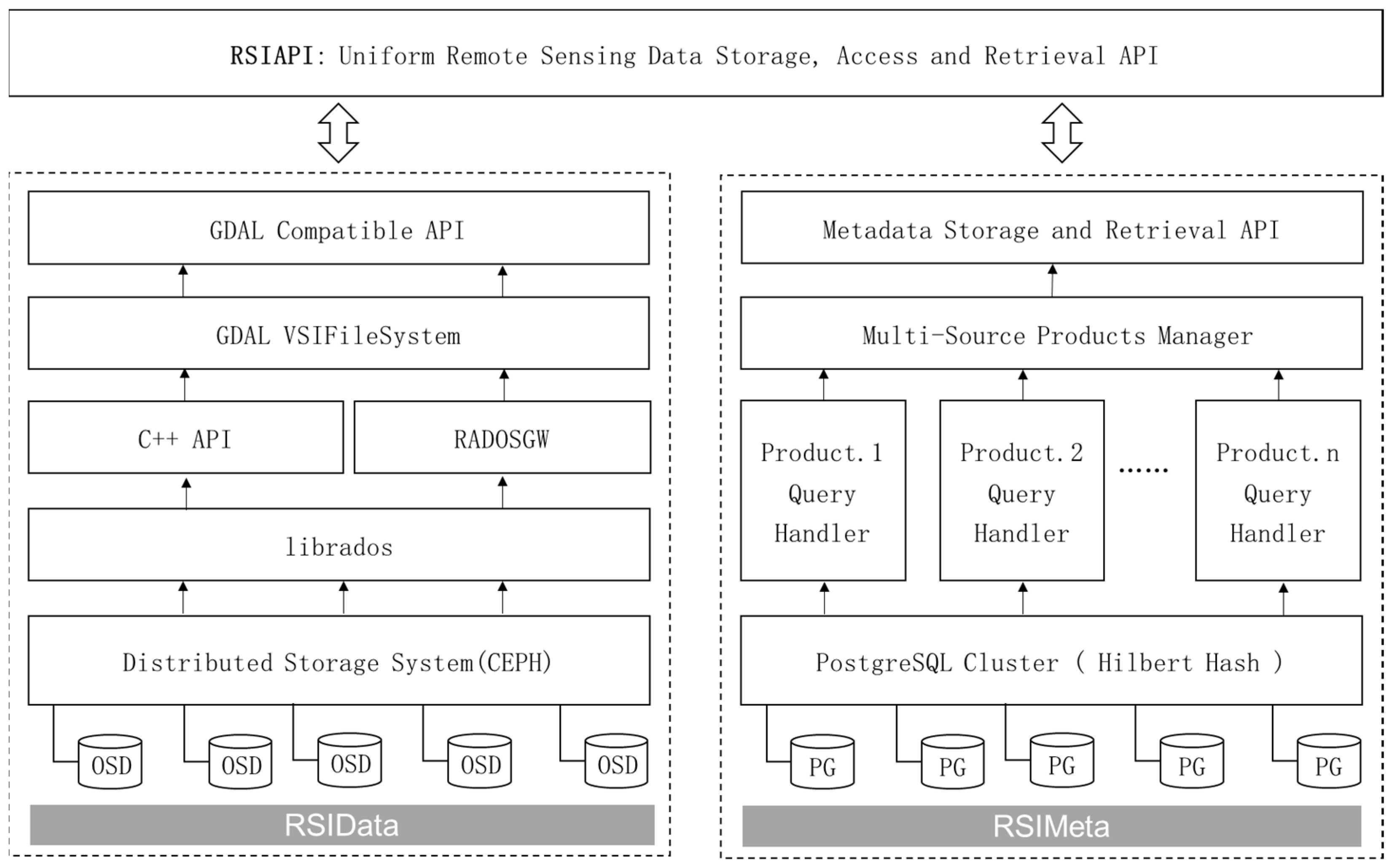
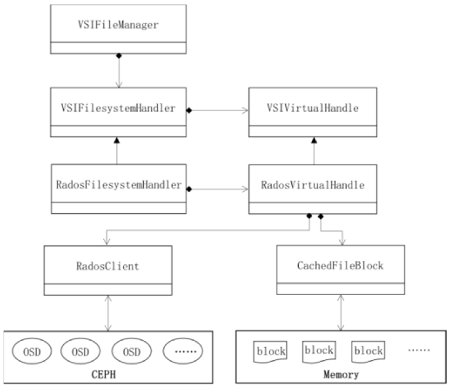
2.3. RSIData: Large-Scale Image Files Storage and GDAL-Compatible Interfaces Design

As introduced in above sections, the amount of remote sensing images is very huge and keeps growing rapidly. An ideal storage system for remote sensing image files should be reliable and scalable. Considering that most applications perform more read operations than write operations, the storage system should support highly concurrent read operations with high performance. Taking all these factors and comparing with different storage systems, we choose CEHP as the remote sensing image files storage system.

CEPH is a kind of distributed object storage system with extraordinary scalability, which can provide petabytes to exabytes storage space based on commodity hardware and intelligent daemons. Compared with other distributed storage systems, the storage location of object in CEPH is computed dynamically based on the CRUSH algorithm [49] rather than looking up tables, which enables the client to communicate with the storage nodes directly without a centralized node. Such a mechanism provides CEPH with high I/O concurrency and performance. Besides that, the CRUSH algorithm can balance the loads of all the storage nodes efficiently, and the loads can be rebalanced quickly if some storage nodes fail, which happens frequently in a very large cluster.

To store and access remote sensing images simply and efficiently, RSIData develops GDAL compatible interfaces on top of CEPH. GDAL (Geospatial Data Abstraction Library) is a translator library for raster and vector formats and provides lots of geospatial command line utilities. GDAL has long being developed for more than 20 years and have large user communities due to its rich features and detailed documents [50]. Based on the abstract raster and vector data models [51,52], GDAL supports over 140+ raster formats, and 80+ vector formats. Nowadays, lots of popular tools and software (ArcGIS, QGIS, rasterio, etc.) support data access through the GDAL library.

Based on the abstract raster data model of GDAL, RSIData provides two types of GDAL compatible interfaces: /vsis3/ and /vsirados/. From the view of geospatial applications, RSIData is abstracted into a virtual filesystem just like NTFS, EXT4, where remote sensing image files can be stored and accessed just like regular files via these interfaces. These interfaces are developed based on librados [53]. Librados is library that allows applications to communicate with CEPH directly using its native communication protocols, and allows users to implement their own customed interfaces.

/vsis3/ is designed for AWS S3 buckets, and has been integrated into the GDAL library. However, applications can access data stored in RSIData with /vsis3/ with the help of RADOSGW, which is an HTTP REST gateway for the RADOS object storage. /vsis3/ interfaces provide a kind of safe and controllable way for remote sensing data share on the Internet. Administrators can limit users to access only the remote sensing data products they have been granted related permissions.

/vsirados/ is another GDAL compatible interface which we implement for better I/O performance and compatibility. Just like /vsis3/, /vsirados/ is implemented based on GDAL virtual filesystem classes, whose inner detailed structure is shown as Figure 20.

VSIFileManager, VSIFilesystemHandler and VSIVirtualHandle are the key abstract classes provided by GDAL library. Storage system inheriting and implementing these classes can be accessed directly by GDAL library.

VSIFileManager is used for new virtual filesystems registration and management. VSIFilesystemHandler and VSIVirtualHandle are the abstract classes for a new virtual filesystem implementation; VSIFilesystemHandler is responsible for file attributes management and directory operations; VSIVirtualHandle is responsible for file data read and write. RadosFilesystemHandler and RadosVirtualHandle are the concrete classes implementing the corresponding abstract classes.

Converting the operations on virtual image file to the real image object in RSIData is implemented in RadosVirtualHandle. For better performance, we added a module, called CachedFileBlock, used for cache frequently visited data blocks in memory. These blocks are parts of remote sensing image files with fixed size. Every block is assigned a unique id generated from the image file and the offset. Considering the limit of memory space, these cached data blocks are regularly updated with the LRU algorithm.

2.4. RSIAPI: Uniform Python Interfaces for Images Storage, Access and Retrieval

The uniform APIs provided by RSIAPI hide the differences of remote sensing image with various structures, making it very simple and straightforward for data access and management. For data administrators, RSIAPI provides a set of management APIs, such as products registration, remote sensing images ingestion, metadata update, etc. For common data users, RSIAPI provides a set of uniform access APIs, such as remote sensing image retrieval, read, write, etc. These APIs are shown as

Table 2. Part of frequently-used APIs provided by RSIAPI.

Package	API	Description
product	Product(*args)	create a Product object from id, title or type
	count(hasfile = None)	return the number of images in the product, and can filter based on whether the image file exists
	filter(expression)	apply the expression to filter the images in the product and return a new Product object including the filtered images
	filterBounds(geometry)	return a new Product object including the images whose spatial area intersects with the geometry
	filterDate(stime, etime)	return a new Product object including the images whose acquisition time between stime and etime
	sort(field, ascending)	sort all images in the product
	first(num = 1)	return the top num Image objects in the images list of the product
	description()	return the detailed description of the product in XML format
image	Image(args)	create a Product object from id
	bands()	return the number of bands in the image
	read(band)	return data of corresponding band file in the type of NumPy Array
	resolution(band)	return the resolution of the image in the unit of meter
	size()	return width and length of the image, represented by the number of pixels
	crs()	return the projected coordinate system in the form of PROJ.4
	geometry(fmt = “GeoJSON”)	return the spatial area in the format of GeoJSON(default) or WKT
	s3path(band)	return the S3 path of image’s band file
	radospath(band)	return the vsirados path of image’s band file
	description()	return the detailed description of the image in XML format
utils	createProduct(**params)	create a new product. Keys of params are the fields of Product table.
	createImage(pid,**params)	create a new image. Keys of params are the fields of Image table.
	search(**params)	retrieve images based on the params. Keys of params are the fields of Image table.
	listProducts()	list all the products in RSIMS

Functions with “*args” or “**params” definitions allow users to pass a variable number of arguments. “**params” is used to pass keyword arguments, and “*args” is used to pass non-keyword arguments.

.

3. Results

In this section, we set up an experimental environment to evaluate the performance of RSIMS, and provided an example to show the usage of RSIMS from the perspective of users. As described in Section 2, RSIMS consists of three modules: RSIMeta, RSIData, and RSIAPI. In the follow-up experiments, we will first verify the spatiotemporal retrieval performance of RSIMeta, and then evaluate the I/O performance of RSIData under different access concurrency. Finally, we provide an example to show how to make a composite Landsat image of China mainland with RSIAPI.

3.1. Experimental Environment Setup

The experimental RSIMS consisted of eight virtual machines provided by a cloud platform. Servers behind the cloud platform are physical machines configured with 8 CPU cores (Intel Xeon E5), 320GB RAM and 80TB HDD. The deployment topology of the experimental RSIMS is shown as Figure 21.

All the virtual machines use Centos 8 operating systems and have the same hardware configuration: 8 CPU cores, 16 GB RAM and 200 GB HDD. These eight machines are located in the same LAN and connected with a Gigabit network.

PGA, PGB and PGC labeled in Figure 21 are used to deploy RSIMeta services. The database used by RSIMeta for metadata management is PostgreSQL V12.2, released on 13 February 2020. Other metadata management and access services are also deployed on these three servers. All the services on PGA, PGB, and PGC are peer to peer. Clients can connect to any one of them for metadata retrieval. As described in Section 2.2.1, 64 databases are distributed across servers based on the Hilbert grids. In this experimental environment, 22 databases with Hilbert codes from 000 to 111 locate in PGA; 21 databases with Hilbert codes from 112 to 222 locate in PGB; 21 databases with Hilbert codes from 223 to 333 locate in PGC. The distribution of these databases is shown as Figure 22.

CephA, CephB, CephC, CephD, and CephE are used to deploy RSIData services. In RSIData, CEPH V15.2.8 is used for the remote sensing image files storage. Other ancillary management and access services are deployed on CephA and CephB. CephA is the primary node, and CehpB serves as the backup node.

Note that this environment is just set up for ease of testing. A typical RSIMS needs dozens of normal virtual machines and high-performance physical machines. The virtual machines with normal configuration usually serve as RSIData servers and high-performance physical machines serve as RSMETA servers.

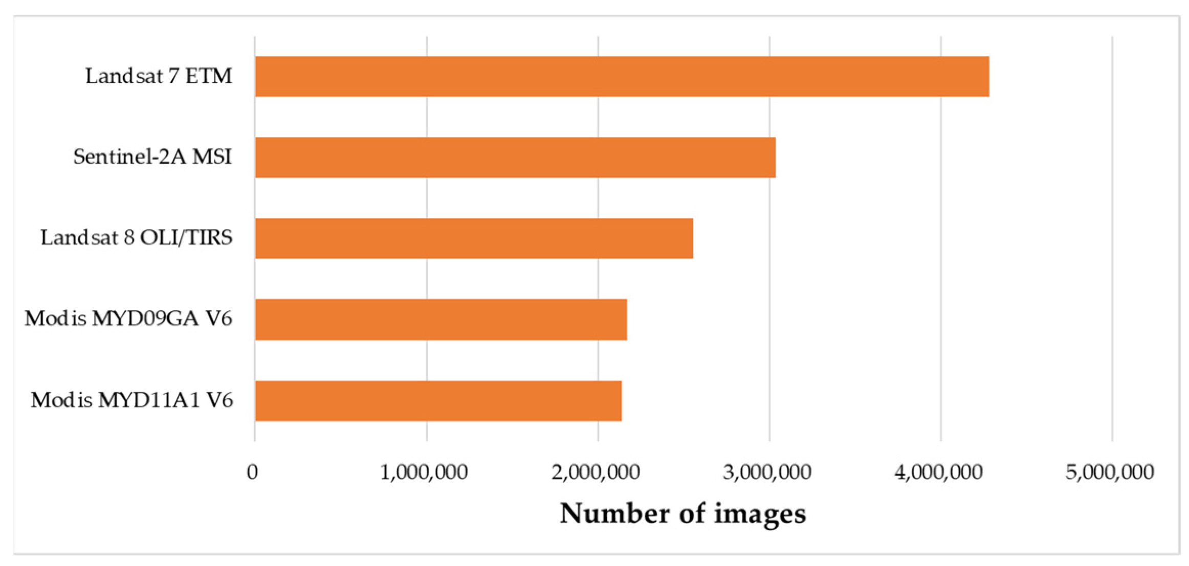
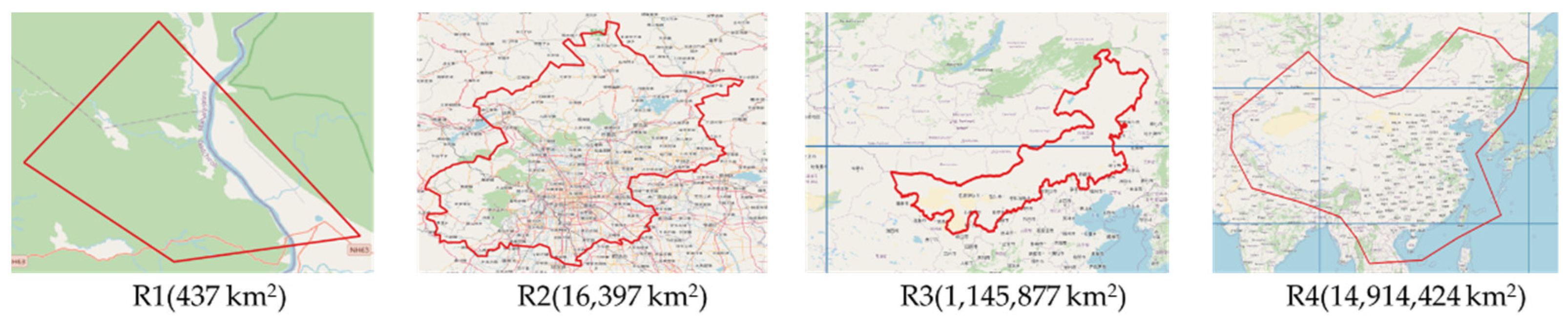
3.2. Experimental Datasets

In this test, we used 14,187,101 images from five datasets with heterogeneous structures. Their basic information has been described in Table 1. The number of images contained in different datasets is shown as Figure 23.

These datasets have been imported into the 64 databases in RSIMeta according to the storage models defined in Section 2.2.3. However, considering the limit of storage capacity provided by RSIData servers, we randomly selected 2000 image binary files and saved them in the RSIData, whose size was 241GB in total.

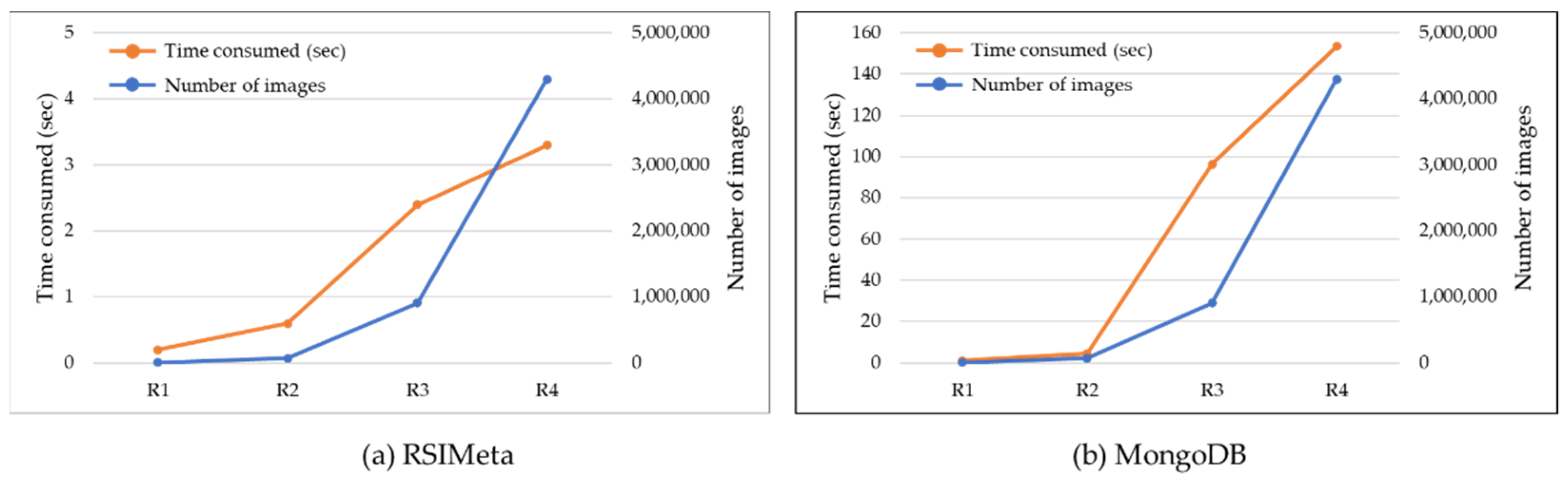
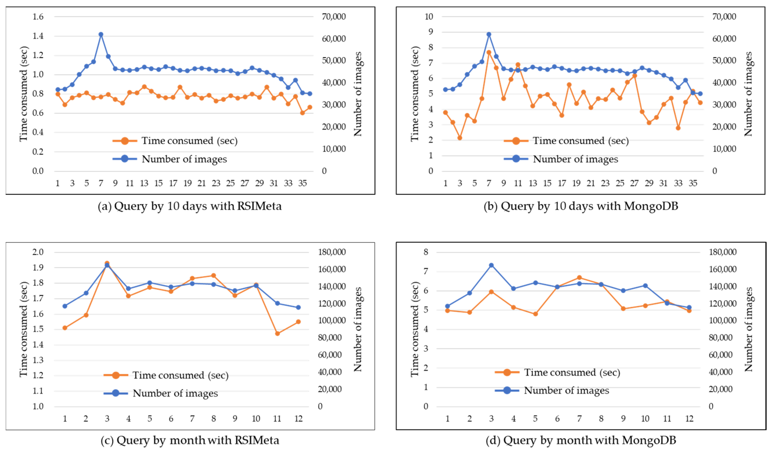
3.3. Spatiotemporal Retrieval Performance of RSIMeta

To verify the performance improved by the Hilbert index algorithm described in Section 2.2.2, we made a comparison of spatiotemporal retrieval performance of RSIMeta and MongoDB in different scenarios. MongoDB is chosen because it is a very popular distributed NOSQL database and provides lots of geospatial functionalities. In MongoDB, geospatial data are stored in the format of GeoJSON. To support efficient geospatial queries, MongoDB provides two types of indexes: 2d index for data stored as points on a two-dimensional plane and 2dsphere index for date stored as GeoJSON objects. A 2dsphere index can handle geospatial queries for inclusion, intersection and proximity with the spatiotemporal functionality: $geoIntersects, $geoWithin, $near and $nearSphere.

In this experiment, we deployed MongoDB (V4.4.2, released on 18 November 2020 by MongoDB, Inc. in New York, NY, USA) in the same servers with RSIMeta and used a sharding method to distribute metadata of images across PGA, PGB and PGC. The data imported into the MongoDB are same with the data from Image table in RSIMeta, and all the geospatial data in MongoDB are indexed with the 2dsphere index.

In order to compare the geospatial query performance, we chose four different polygon regions to perform geospatial intersection query on RSIMeta and MongoDB separately. The regions used in this experiment are shown in Figure 24, denoted by R1, R2, R3, R4.

These four regions locate in different positions and have different sizes. Areas of R1 and R2 regions are relatively small and contained in just a single Hilbert grid (Level 3). So, we can retrieve images intersected with R1 or R2 from a single database. Areas of R3 and R4 are relatively large and cover multiple Hilbert grids (Level 3). Images intersecting with R3 or R4 need to be fetched from multiple databases.

We performed geospatial intersection query on MongoDB and RSIMeta separately. Comparison of time consumed is shown as Figure 25.

From Figure 25, we can find that RSIMeta outperforms significantly MongoDB in the geospatial query scenario. When querying with R1 and R2 regions, the average time consumed by RSIMeta and MongoDB are 0.4 s and 2.8 s separately. When the query area increases from 437 km² to 14,914,424 km² and the number of target images increase from 5707 to 4,309,960, the time consumed by RSIMeta increase from 0.2 s to 3.3 s while the time consumed by MongoDB increase from 1.08 s to 153.5 s. The testing results show that geospatial query efficiency of RSIMeta is very high and stable.

Besides geospatial query, temporal query based on timestamp is another very frequent operation in remote sensing applications. So, the response time in temporal queries is also of very high importance for remote sensing images processing and analysis. Subsequently, we would compare the temporal query performance for RSIMeta versus MongoDB.

Considering that remote sensing images are acquired following a relatively fixed temporal pattern, we chose 1 January 2018~31 December 2018 as the query time window. All the five datasets used by the experiment contain images acquired in this year. Before performing query, we built BTree index on the "atime" field in RSIMeta and MongoDB separately. A comparison of temporal query time consumed is shown as Figure 26.

From the Figure 26, we can see that RSIMeta still outperforms MongoDB in all these temporal query scenarios:

-

The average time consumed of RSIMeta and MongoDB are 0.77 s and 4.64 s respectively when the time window is 10 days.

-

The average time consumed of RSIMeta and MongoDB are 1.7 s and 5.48 s respectively when the time window is a natural month.

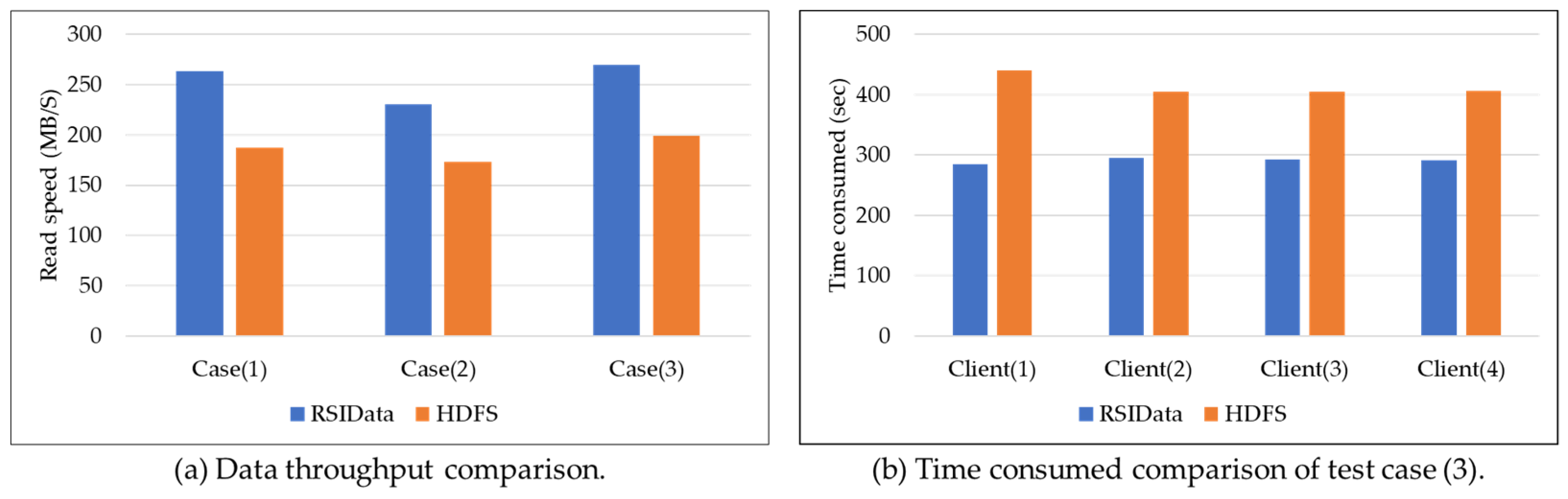
3.4. I/O Performance of RSIData

The main work of RSIData focuses on the efficient and compatible I/O interfaces for remote sensing image files storage and access. As described in Section 2.3, RSIData provides two types of I/O interfaces: /vsis3/ and /vsirados/. Both of them are compatible with GDAL interfaces. Besides that, /vsis3/ is designed to be compatible with AWS S3 for public access from the Internet. /vsirados/ is designed for high I/O performance. In this section, we construct three test cases to verify the I/O performance of RSIData via /vsirados/ interfaces. And another comprehensive example would be provided to show the usage of /vsis3/ in the next section.

To test I/O performance of RSIData, we chose HDFS for comparison. HDFS is a very popular distributed file system, which is not only used to store very large files but also be used as the storage backend for distributed computation systems, such as Hadoop, Spark, etc. Just like the comparison of RSIMeta and MongoDB in Section 3.3, we deployed RSIData and HDFS (V3.2.2, released on 9 January 2021 by the Apache Software Foundation in Wilmington, USA) on the same servers. All the 2000 remote sensing image binary files are imported into RSIData and HDFS separately. As the reference, the speed of copying a file with scp command from any one of these five servers to the client is about 280MB/s.

Considering that RSIData is designed to serve lots of users at the same time, it must be able to cope with mass concurrence access. So, we construct the following three test cases to evaluate its performance with different number of access.

(1) Single I/O process from one client server: Randomly select 100 image files and then read them one by one from RSIData and HDFS separately in the same order.

(2) Twenty concurrent I/O processes from one client server: Randomly select 1000 image files whose size are 20GB in total and then read them simultaneously with 20 processes in parallel.

(3) Eighty concurrent I/O processes from four different client servers: Every server has twenty processes, and all the 2000 image files stored in RSIData are divided into four groups randomly. These processes in different client servers read remote sensing image files in different groups in parallel.

To make the statistical data stable, all the above test cases were executed many times. The final test results are shown as Figure 27.

The right histogram (a) in Figure 27 shows the data throughput comparison between RSIData and HDFS when faced with different number of access. As shown by (a) in Figure 27. RSIData outperforms HDFS in all the test cases. Compared with HDFS, RSIData is closer to the upper limit of network bandwidth(280MB/S), and can transfer more data to clients in the same amount of time. Besides that, the speeds of both RSIData and HDFS don’t change dramatically when the number of access changes. In other words, the increase of access concurrency wouldn’t degrade the performance of RSIData and HDFS, which proves the excellent service stability of RSIData and HDFS.

The left histogram (b) in Figure 27 shows the response time comparison of clients connected to RSIData and HDFS in test case (3). From the histogram(b) in Figure 27, we can find that the response time of clients connected to RSIData are shorter than the clients of HDFS. However, response time of different clients connected to the same system (RSIData or HDFS) are very close. Given the stable performance of RSIData faced with different access concurrency, we can conclude that the response time of clients have negative correlation with the workload of RSIData.

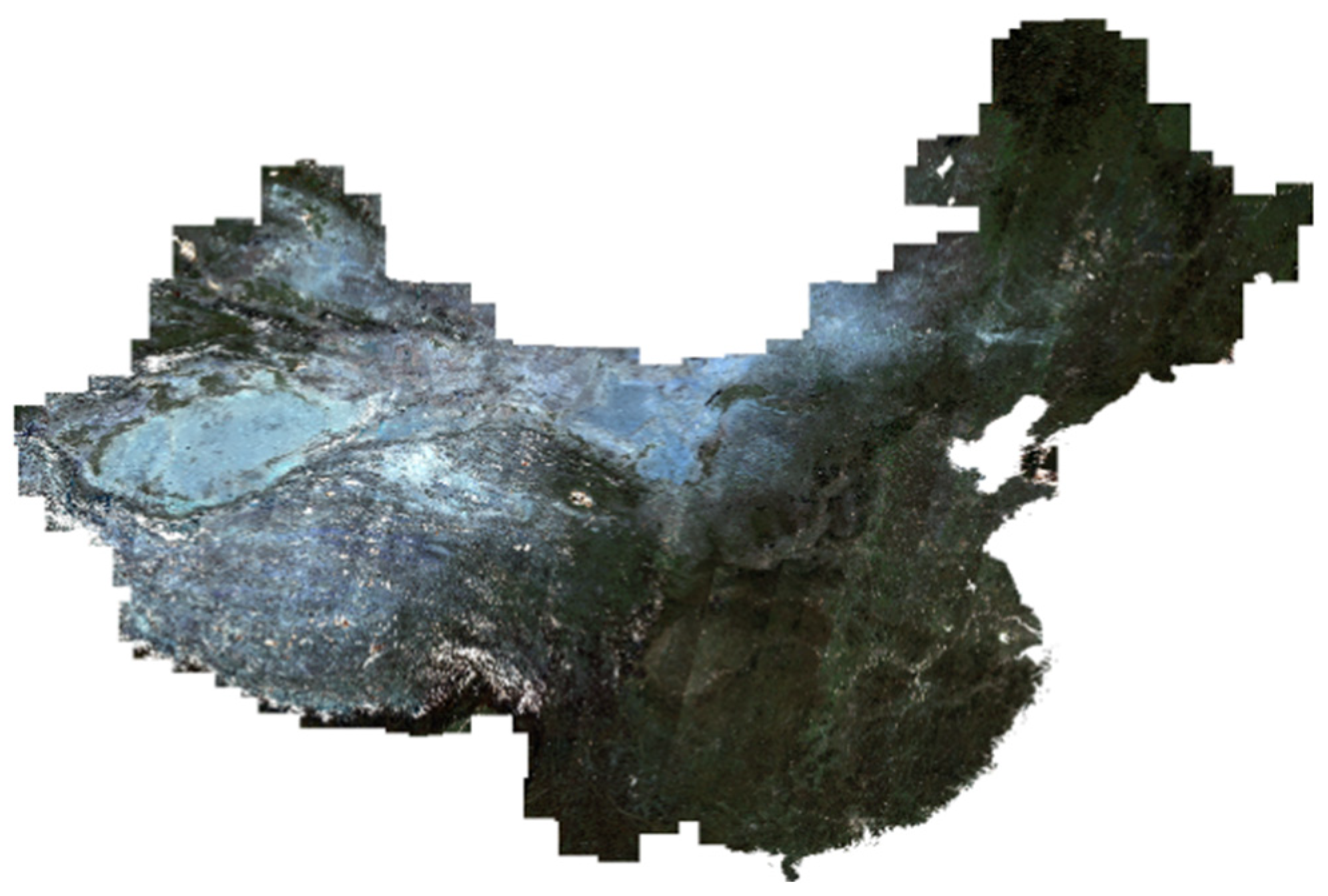
3.5. Example: Make a Composite Landsat Image of China Mainland

In this section, we will provide a comprehensive example to show the basic usage of RSIMS. In this example, we will use Landsat 8 images from 1 May 2019 to 1 October 2019 to make an RGB image covering the mainland of China. The illustrative program is written with Python3, as shown below.

import boto3 import rasterio from rsims import Product from multiprocessing import Pool from rasterio.session import AWSSession session = boto3.Session(aws_access_key_id=access_key, aws_secret_access_key=secret_key) china_image_path = ‘/vsis3/landsat/2019/china.tiff’ with open(“china.geojson”) as f:   geom = f.read() def landsat_moasic(img):   with rasterio.Env(AWSSession(session), **AWS_Options) as env:     with rasterio.open(‘/vsis3/landsat/’+img.b3, ‘r’) as ds:       _b3 = ds.read(1)     with rasterio.open(‘/vsis3/landsat/’+img.b4, ‘r’) as ds:       _b4 = ds.read(1)     with rasterio.open(‘/vsis3/landsat/’+img.b5, ‘r’) as ds:       _b5 = ds.read(1)   landsat_rgb_moasic(china_image_path, _b3, _b4, _b5) prdt = Product( satellite = “landsat”, sensor = “oli/tirs”, type = “c01_t1_sr” ) images = prdt.filterBounds(geom).filterDate(“2019-05-01”, “2019-10-01”) with Pool(processes = 20) as pool:   for img in images:     pool.apply_async(landsat_moasic, (img,))

The first part of the program is used to find the matching images based on the interfaces provided by RSIAPI. These images are retrieved from RSIMeta and then represented by Python3 objects (denoted by Image) whose attributes are constructed from the corresponding item stored in the Image table. Other distinct attributes are dynamically loaded from the corresponding Metadata table. In this example, the search results include 3869 Landsat 8 images intersected with the mainland of China from 1 May 2019 to 1 October 2019, and the total size of these image files is about 460GB.

Bands of the remote sensing image are stored as individual files in the RSIData, and the relative access paths of these image band files are stored as the band attributes of Image objects. As described in above sections, RSIData provides two types of GDAL compatible access methods: /vsirados/ and /vsis3/. The absolute path is composed of the type identification and the relative access path. Take band4 of the image LC08_L1TP_021246_20180413_20180417_01_T1 as the example, its relative path is “/landsat/LC08_L1TP_021246_20180413_20180417_01_T1_B4.TIF”. The corresponding standard S3(Simple Storage Service) path is “/vsis3/landsat/LC08_L1TP_021246_20180413_20180417_01_T1_B4.TIF” and the other type of path is “/vsirados/landsat/LC08_L1TP_021246_20180413_20180417_01_T1_B4.TIF”. In order to speed up the mosaic, we read and process the 3869 images simultaneously with 20 processes. The composite image is shown as Figure 28.

4. Discussion

In the above experiment, we evaluated performance of RSIMS with remote sensing images from different sources, including 14,187,101 image metadata and 2000 image files. The experimental results show the high and stable performance of RSIMS in large amounts of remote sensing images spatial-temporal retrieval and binary files read.

4.1. Spatial-Temporal Retrieval Performance of RSIMS

Metadata of remote sensing images are managed by the RSIMeta module of RSIMS. According to the set of uniform storage models described in Section 2.2.3, all the metadata in RSIMeta are stored in the relational database cluster, which not only provides lots of mature tools for data integration and analysis, but also allows customized optimization based on the data features. In order to improve the spatial-temporal retrieval performance of RSIMeta, we designed a distributed spatial index based on Hilbert curve.

To verify the performance of RSIMeta, we compared it with the MongoDB cluster based on the metadata of 14,187,101 remote sensing images. The experiment results show that RSIMeta is more efficient for large amounts of remote sensing images storage and retrieval. Even deployed in a small cluster with only three virtual machines, it can retrieve millions of remote sensing images intersected with a very large polygon region within less than 10 seconds.

The gain in geospatial query performance of RSIMeta is mainly achieved by three factors: (1) Before performing query, these query regions are subdivided into multi-level Hilbert grids based on the Algorithm 2 described in Section 2.2. These grids are encoded with simple short strings, which are first used to filter lots of images quickly before performing complex geospatial query; (2) These discrete Hilbert codes enable parallel query, and all the involved RSIMeta servers can search the target images simultaneously; (3) Hilbert’s better locality-preserving behavior keeps most of images intersected with a continuous area in the same server, avoiding retrieving data across servers as much as possible. Besides that, the spatial index used by MongoDB is Geohash, which is built based on Z-order curve [54]. Geohash is another public domain geocoding system, and is mainly used to encode the point data to a short string to improve the efficiency of POIs retrieval in a rectangle area.

Take R4 region in Figure 24 as the example, it is divided into 126 grids based on Algorithm 2 before performing geospatial intersection query. These grids filter 8,841,375 images quickly by simple string code matching, and then leave 5,345,726 candidate images for next complex geospatial intersection query. Besides that, R4 covers five big Hilbert grids (201, 202, 230, 231, 232), so the images intersected with R4 clients are saved in five different databases. Based on this information, the client can perform geospatial query simultaneously with five parallel threads. Moreover, three of these five grids locate in the same server (PGC), and most of target images can be retrieved from the same server, reducing the overhead of network communication.

High temporal query performance of RSIMeta benefits from the bottom PostgreSQL cluster. After decades of continuous development and improvement, PostgreSQL has been a very professional database for relational data management. Compared to MongoDB, RSIMeta built on PostgreSQL cluster performs better in temporal query, as shown in Figure 26. Besides that, from the changing trend of (a) and (c) in Figure 26, we can find that time consumed of temporal query in RSIMeta partly depend on the number of target images, whose relationship is positive correlation. However, this positive correlation is not conspicuous in MongoDB. Based on this property, we can distribute data in RSIMeta on more database servers to reduce the data volume in a single database to achieve better retrieval performance.

In a summary, RSIMeta is more suitable than MongoDB for remote sensing image metadata retrieval due to its better spatiotemporal performance.

4.2. Binary Remote Sensing Image Files I/O Performance

Besides the metadata, the other part of remote sensing images are the pixel data stored in binary files. These data are managed in the form of object by the RSIData of RSIMS. The bottom distributed object storage system, CEPH, provides RSIData with excellent capacity scalability and reliability. On top of CEPH, we designed and implemented two I/O interfaces for compatibility with GDAL interfaces and better I/O performance. To verify the I/O performance of RSIData, we compared it with HDFS under different number of concurrent read clients. The results show that RSIData and HDFS are both stable when faced with high concurrent access, but the data transferring speed of RSIData is faster than HDFS.

The I/O performance improvement of RSIData is achieved by two factors: (1) The CRUSH algorithm adopted by CEHP in RSIData can keep large amounts of remote sensing files well balanced across the servers. Based on the algorithm, clients can locate the data address quickly and then read data from the corresponding server directly, which can make full usage of the bandwidth resources of different servers; (2) Some information and data blocks of frequently accessed remote sensing files are cached in the client server with the CachedFileBlock module described in Section 2.3, which reduces the network overload and saves a lot of time.

4.3. Future Work

Work of this paper focus on uniform metadata storage models design, spatial-temporal retrieval performance optimization and GDAL compatible I/O interfaces development. However, some parts of RSIMS still needs to be improved further. The process of different remote sensing image metadata integration is performed manually based on personal knowledge and experience, which can’t ensure that the metadata with different structures can be correctly imported into RSIMeta. To solve the problem, we would conduct more research on the metadata formats and standards of different remote sensing images, and try to make the integration process more automatic. Considering that read operations of remote sensing applications are more frequent than write operations, so we perform more optimizations on data access than data write. In subsequent work, we would optimize write and update operations for better performance. Besides that, I/O interfaces would be extended further to provide better support for remote sensing applications, such as reading data by geospatial regions, exporting raster files to images, etc. Combining with popular distributed computing systems (e.g., Spark, Hadoop) to achieve better process and analysis efficiency is another important research direction.

5. Conclusions

With the rapid development of remote sensing technology, remote sensing data keep growing explosively, and play a more and more important role in environmental protection, economic development, etc. However, managing such huge amounts of remote sensing data is still a big challenge. Besides the large volume, big remote sensing data have many specific features, such as multi-scale, high-dimension, spatiotemporal pattern, etc. Moreover, metadata of remote sensing images from different sources vary greatly. Traditional storage systems are inappropriate to be used directly for big remote sensing data management.

Faced with these challenges, we designed and implemented the remote sensing image management system (RSIMS), a new distributed remote sensing data storage system. RSIMS adopts a modular and layered architecture, which is composed of RSIAPI, RSIMeta and RSIData modules. Structured text metadata and unstructured binary file data of remote sensing images are managed by RSIMeta and RSIData separately. RSIMeta stores all the metadata extracted from different remote sensing images according to the uniform storage models, and then builds a distributed spatial index based on Hilbert curve for better spatiotemporal retrieval performance. Up to now, RSIMeta has integrated about 100 million remote sensing images and can retrieve millions of remote sensing images intersected with a large geospatial region within 10 seconds; RSIData is a distributed remote sensing image file storage system with large scalable capacity and high I/O performance. In order to be compatible with GDAL programs, RSIData provides two types of I/O interfaces, which can be used to access remote sensing image files directly stored in RSIData by most of popular related tools and software. On top of them, RSIAPI provides a set of uniform Python APIs for remote sensing applications, hiding the complex inner storage structures from the users. Finally, comparative experiments prove the high and stable performance of RSIMS for large-scale remote sensing image storage, access, and retrieval.

Some work has been left for the future due to a lack of time. First, we would conduct more research on remote sensing data formats and standards, and then improve the metadata models to make the data integration process more automatic and accurate. Besides that, we would continue to extend and optimize I/O interfaces of RSIMS to provide better support for remote sensing applications and combine with popular distributed computing systems to achieve better process ana analysis efficiency.

References

1. Remote Sensing: Introduction and History. Available online: https://earthobservatory.nasa.gov/features/RemoteSensing (accessed on 23 April 2021).
2. Big Data. Available online: http://www.gartner.com/it-glossary/big-data (accessed on 1 February 2021).
3. DigitalGlobe Satellite and Product Overview. Available online: https://calval.cr.usgs.gov/apps/sites/default/files/jacie/DigitalGlobeOverview_JACIE_9_19_17.pdf (accessed on 1 February 2021).
4. Grawinkel, M.; Nagel, L.; Padua, F.; Masker, M.; Brinkmann, A.; Sorth, L. Analysis of the ECMWF storage landscape. In Proceedings of the 13th USENIX Conference on File and Storage Technologies, Santa Clara, CA, USA, 15–19 February 2015; p. 83. [Google Scholar]
5. Guo, C.-l.; Zhao, Y. Research on Application of Blockchain Technology in Field of Spatial Information Intelligent Perception. Comput. Sci. 2020, 47, 354–358, 362. [Google Scholar]
6. Fan, J.; Yan, J.; Ma, Y.; Wang, L. Big Data Integration in Remote Sensing across a Distributed Metadata-Based Spatial Infrastructure. Remote Sens. 2018, 10, 7. [Google Scholar] [CrossRef] [Green Version]
7. Hansen, M.C.; Potapov, P.V.; Moore, R.; Hancher, M.; Turubanova, S.A.; Tyukavina, A.; Thau, D.; Stehman, S.V.; Goetz, S.J.; Loveland, T.R.; et al. High-Resolution Global Maps of 21st-Century Forest Cover Change. Science 2013, 342, 850–853. [Google Scholar] [CrossRef] [PubMed] [Green Version]
8. Gibson, R.; Danaher, T.; Hehir, W.; Collins, L. A remote sensing approach to mapping fire severity in south-eastern Australia using sentinel 2 and random forest. Remote Sens. Environ. 2020, 240, 111702. [Google Scholar] [CrossRef]
9. Weiss, M.; Jacob, F.; Duveiller, G. Remote sensing for agricultural applications: A meta-review. Remote Sens. Environ. 2020, 236, 111402. [Google Scholar] [CrossRef]
10. Wang, F.; Oral, S.; Shipman, G.; Drokin, O.; Wang, T.; Huang, I. Understanding Lustre Filesystem Internals; Technical Paper; Oak Ridge National Laboratory, National Center for Computational Sciences: Oak Ridge, TN, USA, 2009. [Google Scholar]
11. Ghemawat, S.; Gobioff, H.; Leung, S.-T. The Google file system. In Proceedings of the 19th ACM Symposium on Operating Systems Principles, Bolton Landing, NY, USA, 19–22 October 2003. [Google Scholar]
12. Dana, P.; Silviu, P.; Marian, N.; Marc, F.; Daniela, Z.; Radu, C.; Adrian, D. Earth observation data processing in distributed systems. Informatica 2010, 34, 463–476. [Google Scholar]
13. Qiao, X. The distributed file system about moose fs and application. Inspur 2009, 5, 9–10. [Google Scholar]
14. Weil, S.A.; Brandt, S.A.; Miller, E.L.; Long, D.D.E.; Maltzahn, C. Ceph: A scalable, high-performance distributed file system. In Proceedings of the 7th Symposium on Operating Systems Design and Implementation, Seattle, WA, USA, 6–8 November 2006. [Google Scholar]
15. Li, H.; Ghodsi, A.; Zaharia, M.; Shenker, S.; Stoica, I. Tachyon: Reliable, memory speed storage for cluster computing frameworks. In Proceedings of the ACM Symposium on Cloud Computing, Seattle, WA, USA, 3–5 November 2014. [Google Scholar]
16. Beaver, D.; Kumar, S.; Li, H.C.; Sobel, J.; Vajgel, P. Finding a needle in Haystack: Facebook’s photo storage. In Proceedings of the Usenix Conference on Operating Systems Design & Implementation, Vancouver, ON, Canada, 4–6 October 2010. [Google Scholar]
17. Ma, Y.; Wang, L.; Zomaya, A.; Chen, D.; Ranjan, R. Task-tree based large-scale mosaicking for massive remote sensed imageries with dynamic DAG scheduling. IEEE Trans. Parallel Distrib. Syst. 2014, 25, 2126–2137. [Google Scholar] [CrossRef]
18. Kou, W.; Yang, X.; Liang, C.; Xie, C.; Gan, S. HDFS enabled storage and management of remote sensing data. In Proceedings of the 2016 2nd IEEE International Conference on Computer and Communications (ICCC 2016), Chengdu, China, 14–17 October 2016; pp. 80–84. [Google Scholar]
19. Wang, P.; Wang, J.; Chen, Y.; Ni, G. Rapid processing of remote sensing images based on cloud computing. Future Gener. Comput. Syst. 2013, 29, 1963–1968. [Google Scholar] [CrossRef]
20. Almeer, M.H. Cloud Hadoop Map Reduce for Remote Sensing Image Analysis. J. Emerg. Trends Comput. Inf. Sci. 2014, 4, 637–644. [Google Scholar]
21. Gorelick, N.; Hancher, M.; Dixon, M.; Ilyushchenko, S.; Thau, D.; Moore, R. Google Earth Engine: Planetary-scale geospatial analysis for everyone. Remote Sens. Environ. 2017, 202, 18–27. [Google Scholar] [CrossRef]
22. Earth on AWS. Available online: https://aws.amazon.com/earth (accessed on 1 February 2021).
23. R-tree. Available online: https://en.wikipedia.org/wiki/R-tree (accessed on 1 February 2021).
24. Peano, G. Sur une courbe, qui remplit toute une aire plane. In Arbeiten zur Analysis und zur Mathematischen Logik; Springer: Vienna, Austria, 1990. [Google Scholar]
25. March, V.; Yong, M.T. Multi-Attribute Range Queries on Read-Only DHT. In Proceedings of the 15th International Conference on Computer Communications and Networks (ICCCN), Arlington, VA, USA, 9–11 October 2006. [Google Scholar]
26. Huang, Y.-K. Indexing and querying moving objects with uncertain speed and direction in spatiotemporal databases. J. Geogr. Syst. 2014, 16, 139–160. [Google Scholar] [CrossRef]
27. Zhang, R.; Qi, J.; Stradling, M.; Huang, J. Towards a painless index for spatial objects. ACM Trans. Database Syst. 2014, 39, 1–42. [Google Scholar] [CrossRef]
28. Nivarti, G.V.; Salehi, M.M.; Bushe, W.K. A mesh partitioning algorithm for preserving spatial locality in arbitrary geometries. J. Comput. Phys. 2015, 281, 352–364. [Google Scholar] [CrossRef]
29. Xia, X.; Liang, Q. A GPU-accelerated smoothed particle hydrodynamics (SPH) model for the shallow water equations. Environ. Model. Softw. 2016, 75, 28–43. [Google Scholar] [CrossRef]
30. Herrero, R.; Ingle, V.K. Space-filling curves applied to compression of ultraspectral images. Signal Image Video Process. 2015, 9, 1249–1257. [Google Scholar] [CrossRef]
31. Wang, L.; Ma, Y.; Zomaya, A.Y.; Ranjan, R.; Chen, D. A parallel file system with application-aware data layout policies for massive remote sensing image processing in digital earth. IEEE Trans. Parallel Distrib. Syst. 2015, 26, 1497–1508. [Google Scholar] [CrossRef]
32. Hilbert, D. Über die stetige Abbildung einer Linie auf ein Flächenstück. Mathematische Annalen 1891, 38, 459–460. [Google Scholar] [CrossRef] [Green Version]
33. Weisstein, E.W. Sierpiński Curve. Available online: https://en.wikipedia.org/wiki/MathWorld (accessed on 5 April 2021).
34. Avdoshin, S.M.; Beresneva, E.N. The Metric Travelling Salesman Problem: The Experiment on Pareto-optimal Algorithms. Proc. ISP RAS 2017, 29, 123–138. [Google Scholar] [CrossRef] [Green Version]
35. Meister, O.; Rahnema, K.; Bader, M. Parallel memory-efficient adaptive mesh refinement on structured triangular meshes with billions of grid cells. ACM Trans. Math. Software 2016, 43, 1–27. [Google Scholar] [CrossRef]
36. Mokbel, M.F.; Aref, W.G.; Kamel, I. Analysis of Multi-Dimensional Space-Filling Curves. GeoInformatica 2003, 7, 179–209. [Google Scholar] [CrossRef]
37. Moon, B.; Jagadish, H.; Faloutsos, C.; Saltz, J.H. Analysis of the Clustering Properties of Hilbert Space-filling Curve. IEEE Trans. Knowl. Data Eng. 2001, 13, 124–141. [Google Scholar] [CrossRef] [Green Version]
38. Jagadish, H.V. Linear clustering of objects with multiple attributes. In Proceedings of the 1990 ACM SIGMOD International Conference on Management of data, Atlantic City, NJ, USA, 23–25 May 1990. [Google Scholar]
39. ANZLIC. ANZLIC Working Group on Metadata: Core Metadata Elements; Australia and New Zealand Land Information Council: Sydney, Australia, 1995. [Google Scholar]
40. FGDC. FGDC-STD-001-1998—Content Standard for Digital Geographic Metadata; Federal Geographic Data Committee: Washington, DC, USA, 1998; p. 78. [Google Scholar]
41. Moellering, H.; Aalders, H.; Crane, A. World Spatial Metadata Standards; Elsevier Ltd.: London, UK, 2005; p. 689. [Google Scholar]
42. Brodeur, J.; Coetzee, S.; Danko, D.; Garcia, S.; Hjelmager, J. Geographic information metadata—an outlook from the international standardization perspective. ISPRS Int. J. Geo. Inf. 2019, 8, 280. [Google Scholar] [CrossRef] [Green Version]
43. ISO/TC 211. ISO19115:2003. Geographic Information—Metadata; International Organization for Standardization: Geneva, Switzerland, 2003. [Google Scholar]
44. ISO/TC 211. ISO19115-2:2009. Geographic Information—Metadata—Part 2: Extensions for Imagery and Gridded Data; International Organization for Standardization: Geneva, Switzerland, 2009. [Google Scholar]
45. ISO/TC 211. ISO19115-2:2019. Geographic Information—Metadata—Part 2: Extensions for Acquisition and Processing; International Organization for Standardization: Geneva, Switzerland, 2019. [Google Scholar]
46. Unified Metadata Model (UMM). Available online: https://earthdata.nasa.gov/eosdis/science-system-description/eosdis-components/cmr/umm (accessed on 7 April 2021).
47. van der Veen, J.S.; Sipke, J.; van der Waaij, B.; Meijer, R.J. Sensor data storage performance: SQL or NoSQL, physical or virtual. In Proceedings of the 5th IEEE International Conference on Cloud Computing, Honololu, HI, USA, 24–29 June 2012. [Google Scholar]
48. Makris, A.; Tserpes, K.; Spiliopoulos, G.; Anagnostopoulos, D. Performance Evaluation of MongoDB and PostgreSQL for Spatio-temporal Data. In Proceedings of the EDBT/ICDT 2019 Joint Conference on CEUR-WS.org, Lisbon, Portugal, 26 March 2019. [Google Scholar]
49. Weil, S.A.; Brandt, S.A.; Miller, E.L.; Maltzahn, C. CRUSH: Controlled, Scalable, Decentralized Placement of Replicated Data. In Proceedings of the 2006 ACM/IEEE Conference on Supercomputing, Tampa, FL, USA, 11–17 November 2006. [Google Scholar]
50. Coverity Scan: GDAL. Available online: https://scan.coverity.com/projects/gdal (accessed on 1 February 2021).
51. Raster Data Model. Available online: https://gdal.org/user/raster_data_model.html (accessed on 1 February 2021).
52. Vector Data Model. Available online: https://gdal.org/user/vector_data_model.html (accessed on 1 February 2021).
53. Introduction to Librados. Available online: https://docs.ceph.com/en/latest/rados/api/librados-intro (accessed on 7 April 2021).
54. 2nd Index Internals. Available online: https://docs.mongodb.com/manual/core/geospatial-indexes (accessed on 7 April 2021).
Figure 1. The overall architecture of RSIMS.
Remotesensing 13 01815 g001
Figure 2. Typical space-filling curves.
Remotesensing 13 01815 g002
Figure 3. Jump and Contiguity percentages comparison of Hilbert curve, Gray curve and Z-order curve.
Remotesensing 13 01815 g003
Figure 4. Basic global Hilbert grids.
Remotesensing 13 01815 g004
Figure 5. Structure of two-tier distributed spatial index.
Remotesensing 13 01815 g005
Figure 6. Basic shapes of Hilbert curve.
Remotesensing 13 01815 g006
Figure 7. Transition matrixes for Hilbert curves.
Remotesensing 13 01815 g007
Figure 8. Remote sensing image encoding and storage.
Remotesensing 13 01815 g008
Figure 9. Relationship of S, B and G.
Remotesensing 13 01815 g009
Figure 10. Grids generated from Algorithm 2 are not consistent with standard Hilbert grids.
Remotesensing 13 01815 g010
Figure 11. Process of grids merges according to Hilbert curve.
Remotesensing 13 01815 g011
Figure 12. Remote sensing images parallel query based on Hilbert grids.
Remotesensing 13 01815 g012
Figure 13. Problems of spatial query based on Hilbert grids.
Remotesensing 13 01815 g013
Figure 14. Overall metadata structure of ISO 19115-2.
Remotesensing 13 01815 g014
Figure 15. Mapping from Landsat property to ISO 19115 property.
Remotesensing 13 01815 g015
Figure 16. Overall storage schema of RSIMeta.
Remotesensing 13 01815 g016
Figure 17. Structure of Product table.
Remotesensing 13 01815 g017
Figure 18. Structure of Image table.
Remotesensing 13 01815 g018
Figure 19. The flow of multi-source heterogeneous remote sensing images integration.
Remotesensing 13 01815 g019
Figure 20. Detailed structure of /vsirados/ implementation.
Remotesensing 13 01815 g020
Figure 21. Deployment topology of the experimental RSIMS.
Remotesensing 13 01815 g021
Figure 22. Databases distribution based on Hilbert grids.
Remotesensing 13 01815 g022
Figure 23. Number of remote sensing images from different sources.
Remotesensing 13 01815 g023
Figure 24. Query regions with different sizes.
Remotesensing 13 01815 g024
Figure 25. Comparison of geospatial time consumed based on R1, R2, R3 and R4.
Remotesensing 13 01815 g025
Figure 26. Comparison of temporal query time consumed based on different time windows. Time windows of (a,b) are 10 days; Time windows of (c,d) is the natural months (from January to December).
Remotesensing 13 01815 g026
Figure 27. Performance comparison of RSIData and HDFS.
Remotesensing 13 01815 g027
Figure 28. The composite Landsat image of China mainland.
Remotesensing 13 01815 g028