Article

Study on Radar Echo-Filling in an Occlusion Area by a Deep Learning Algorithm

1
School of Atmospheric Sciences, Chengdu University of Information Technology, Chengdu 610225, China
2
State Key Lab of Severe Weather, Chinese Academy of Meteorological Sciences, Beijing 100081, China
*
Author to whom correspondence should be addressed.
Remote Sens. 2021, 13(9), 1779; https://doi.org/10.3390/rs13091779
Submission received: 18 March 2021 / Revised: 28 April 2021 / Accepted: 29 April 2021 / Published: 2 May 2021

Abstract

:
Radar beam blockage is an important error source that affects the quality of weather radar data. An echo-filling network (EFnet) is proposed based on a deep learning algorithm to correct the echo intensity under the occlusion area in the Nanjing S-band new-generation weather radar (CINRAD/SA). The training dataset is constructed by the labels, which are the echo intensity at the 0.5° elevation in the unblocked area, and by the input features, which are the intensity in the cube including multiple elevations and gates corresponding to the location of bottom labels. Two loss functions are applied to compile the network: one is the common mean square error (MSE), and the other is a self-defined loss function that increases the weight of strong echoes. Considering that the radar beam broadens with distance and height, the 0.5° elevation scan is divided into six range bands every 25 km to train different models. The models are evaluated by three indicators: explained variance (EVar), mean absolute error (MAE), and correlation coefficient (CC). Two cases are demonstrated to compare the effect of the echo-filling model by different loss functions. The results suggest that EFnet can effectively correct the echo reflectivity and improve the data quality in the occlusion area, and there are better results for strong echoes when the self-defined loss function is used.

1. Introduction

Weather radar is an important means of cloud precipitation physics research and precipitation monitoring and early warning. It is widely used in meteorological operational observations and research. Radar detection capability is affected not only by the radar hardware parameters but also by the topography and tall buildings around the radar station [1]. Terrain blockage results in a radar observation blind area, which causes a reduction in the radar beam power and further influences the multiradar mosaic and other radar secondary products, such as quantitative precipitation estimation (QPE), which depends on echo intensity [2,3]. Therefore, blocking correction is important to improve the accuracy of quantitative detection of weather radar.
At present, many beneficial studies have been performed on radar beam blocking. For example, beam blockage correction is based on a high-precision digital elevation model (DEM). The DEM is a kind of terrain model that expresses the spatial distribution of ground elevation. The DEM-based beam blockage correction method was based on the equations of radar beam propagation in a standard atmosphere proposed by Battan [4]. Some scholars correct reflectivity bias over the blockage zone by calculating the power loss of beam shielding in a standard atmosphere [5,6,7]. According to the occlusion rate calculated by the DEM, a filling method using the average value of gates is proposed, which can correct the echo data in the azimuth of a small blocking coefficient using the adjacent plan position indicator (PPI) in real time [8]. A correction method of partial beam blockage is discussed according to the valid data area calculated by the DEM in the constant altitude plan position indicator (CAPPI) [9]. Shakti et al. [10] proposed a modified DEM method by means of simply calculating the power loss of the received signal because of ground clutter, hardware calibration errors, etc. However, the above DEM-based beam blockage correction methods are mainly based on standard atmospheric conditions, which are not suitable for blockage correction of super-refraction. Furthermore, the emergence of new buildings and trees causes additional beam blocking, which makes it difficult to update DEM data in time. Therefore, some echo correction models that do not rely on DEMs have been addressed recently. Gou et al. [11] proposed a blocking region identification algorithm based on the echo probability features and not dependence on DEM, in which the partial occlusion echoes are removed first and then corrected with multiradar mosaic data to eliminate the discontinuity of echo. According to the spatial correlation in adjacent azimuths, the echo data in adjacent radial and upper elevations are used for occlusion correction and linear interpolation is performed for partial occlusion or complete occlusion in a small area [12].
In addition, the vertical profiles of reflectivity (VPR) are utilized in beam blockage correction [13,14]. The mesoscale VPR retrieved by rainfall data within 70 km and by radar reflectivity are performed to correct the blockage, and the correction scheme is verified by comparing radar QPE with gauge measurements [15]. An optimal match method is suggested on the basis of the echo uniformity to calculate the VPR in different areas. The VPR in the occlusion area is matched with the average VPR in multiple nonocclusion areas, and these average VPRs are further matched with rain gauges to obtain the optimal reflectivity, which is utilized to fill the blocking echo corresponding to the gauges [16]. There are other VPR correction methods according to the occlusion orientation and degree calculated by the DEM. Andrieu et al. [17] and Creutin et al. [18] divided radar volume scan data into blocked and unblocked areas by means of the DEM and corrected the reflectivity in the blocked area with VPR generated from the unblocked areas. The echoes in low-elevation, completely blocked areas are filled by the data in high-elevation, unblocked areas using the statistical analysis of VPR, and the filling effect is evaluated by contrasting the reflectivity factor and radar QPE values before and after filling [19]. However, most of the above VPR technology is focused on large-scale precipitation processes dominated by stratiform clouds, the VPR correction method has its shortage since there are poor relationship between upper and lower reflectivity in an isolated convective storm with uneven internal distribution.
In recent years, artificial intelligence (AI) has been developing rapidly. In contrast to the traditional meteorological analysis method, deep learning, as the main AI algorithm, has an obvious advantage in dealing with nonlinear problems. Many studies have been performed with deep learning in the meteorological field, such as cloudage nowcasting [20], cloud-type classification [21], tropical cyclone intensity estimation [22], etc. Moreover, weather radar is a major means to examine the intensity of precipitation and distribution of weather systems, and combining it with a deep learning algorithm to process it will effectively improve rain nowcasting [23]. Recurrent neural networks (RNNs) are employed to capture spatiotemporal correlations from radar echo spatiotemporal sequences to obtain extrapolation vectors and to further predict the development and movement of radar echoes [24,25]. Tran et al. [26] presented an investigation into the problem of 3D radar echo extrapolation in precipitation nowcasting with recent AI advances and computer vision technology. Two neural network-based architectures, namely, a radar mosaic-based convolutional neural network (RMCNN) and a radar mosaic-based multilayer perceptron (RMMLP), are proposed to estimate typhoon rainfall [27]. Bouget et al. [28] trained a deep learning model on a fusion of rainfall radar images and wind velocity produced by a weather forecast model to determine whether using other meteorological parameters such as wind would improve forecasts.
The paper is organized as follows. In Section 2 of this paper, the construction steps of the training dataset are introduced in detail, which include data sources, preprocessing, and range splitting skills. In Section 3, an echo-filling network (EFnet) is proposed, which includes model network architecture design, self-defined loss function improvement, and hyperparameter setting. Six models are built by means of a training dataset and EFnet network. Two cases are tested to verify the filling models in Section 4. Finally, a summary and discussion of radar applications based on deep learning algorithms are presented in Section 5.

2. Construction of the Training Dataset

2.1. Data Sources

The radar data are observed with the Nanjing S-band new-generation Doppler weather radar (CINRAD/SA). The radar operates with a spatial resolution of 1 km × 1°, and maximum detection range of 460 km, and it works with the volume scan mode of VCP21, which is performed every 6 min and 9 elevation layers (0.5°, 1.5°, 2.5°, 3.5°, 4.5°, 6.0°, 10.0°, 15.0°, and 19.5°). As shown in Figure 1, due to the influence of the surrounding geographical environment, there is serious terrain blockage in azimuths from 132° to 137° and from 220° to 233° in the 0.5° elevation. The maximum blockage rate is larger than 0.75, and beam occlusion disappears with radar antenna lifting.

2.2. Data Preprocessing

Data cleaning is a key process to ensure model accuracy and effectiveness before the training dataset is constructed. The quality control of radar base data is implemented to eliminate the pollution of ground clutter and other non-meteorological echoes [29,30]. Some thresholds which include echo intensity, radial velocity, and the vertical gradient of echo intensity are used to reduce the misjudgment of the meteorological echo [31]. The deep learning training dataset consists of labels and feature data. The labels are the conclusion that needs to be obtained, in which are the echo intensity at 0.5° elevation, and the feature data are the evidence for correction, in which are the intensity at the upper elevation corresponding to the location of labels. Therefore, atmospheric refraction should be considered when the ranges at different elevation angles are calculated.
In the ideal state, the electromagnetic wave propagates along a straight line. However, the propagation path is curved because of the uneven distribution of the refractive index in the atmosphere, which is the results of variation in temperature, pressure, and humidity with the height (Figure 2). To simplify the calculation, an equivalent earth radius is applied to support radar beam propagation as a straight line [32]. The relationship between the equivalent earth radius R′ and atmospheric refractive index n is:
R = R 1 + R d n d h ,
where R is the radius of earth (R = 6371 km) and h is the height of the radar beam from the ground. In the standard atmosphere, dn/dh is taken as −4 × 10⁻⁸ m−1, and Equation (1) is simplified as R′ ≈ 4/3 R. Therefore, the number of radial gates corresponding to each scan layer can be calculated as:
G = ( R + h 0 ) sin α r cos ( α + β ) ,
where G is the gate number, h0 is the antenna height from the ground, α is the equivalent geocentric angle (α = 4/3 a, where a is the geocentric angle), β is the elevation angle, and r is the radial resolution (r = 1 km). Through Equation (2), the reflectivity values at 0.5° elevation can be obtained as labels, and N × 3 × 3 values within 3 radials, 3 gates, and N scan layers corresponding to the location of labels are outputted as features of the training dataset.
The reflectivity value is set to −20 dBZ when it is less than the radar detection sensitivity of −5 dBZ. If the value of the tag is −20 dBZ, this gate is not outputted into the training dataset. On the other hand, the data are also not appended to the dataset when all feature values are −20 dBZ. Then, the data are normalized into [0,1] by the min-max standardization method:
y = y min max min ,
where y and y′ are the true and normalized values, respectively; the value of min is set to −20 dBZ, and the value of max is set to 70 dBZ.

2.3. Building the Training Dataset

Considering that the radar beam broadens with distance and altitude, only data within 150 km are built as models. The range in 0.5° elevation is divided into six sections each 25 km, i.e., from 1 to 25, 25 to 50, 50 to 75, 75 to 100, 100 to 125, and 125 to 150 km. It can be seen from Figure 1 that the unblocked areas include azimuths from 0° to 90° and 300° to 360° in the Nanjing radar, so the two nonocclusion areas are selected to construct a training dataset of deep learning, where the echo reflectivity at 0.5° elevation is taken as the labels, the reflectivity of N × 3 × 3 points consisting of 3 radials, 3 gates, and N scan layers are the input features, and N equals to 7, 6, 5, 4, 3, or 2 according to the distance of the section to the radar.
A total of 114 volume scan data from April to July, 2012–2017, was selected, which is the rainy season in Nanjing. The data sizes in the six sections are listed in Table 1, which are split into a training set and a test set of 80% and 20% to build and test the echo-filling models, respectively.

3. Building the Echo-Filling Model

3.1. Model Network Architecture Design

Deep learning is also called a multilayer neural network. Its basic architecture includes an input layer, multiple hidden layers, and an output layer. Activation functions are invented to solve the problem of gradient disappearance or explosion caused by too many hidden layers. The common activation functions include the sigmoid function, tanh, softmax, and ReLU. By means of the activation function, hidden layers, and nodes in each hidden layer, the neural network can fit a very complex nonlinear model and can describe a more detailed mapping relationship.
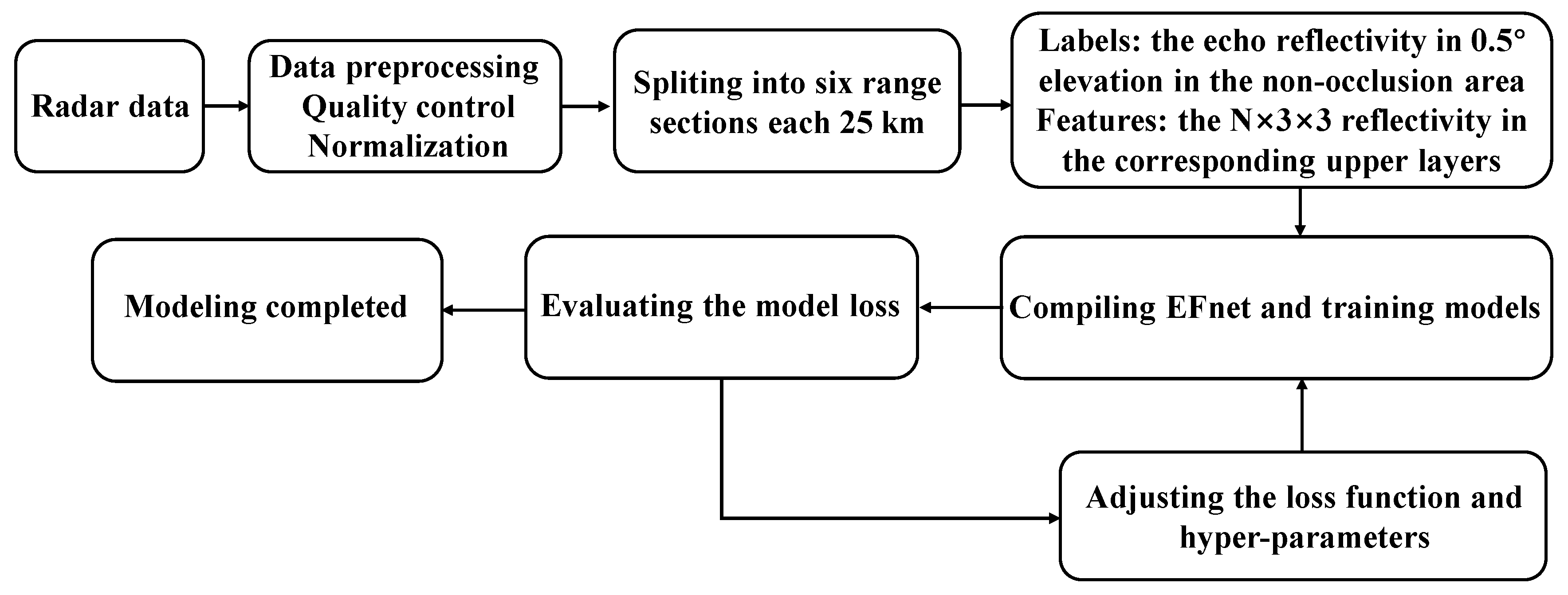
Considering fitting speed and effect, an EFnet is designed with three linear hidden layers after many tests. To avoid overfitting and enhance the generalization ability of the model, a dropout layer is added in each hidden layer, in which 20% of neurons are randomly discarded in each linear layer during forward propagation. The active functions select ReLU and sigmoid. The architecture of EFnet is shown in Figure 3 and the modeling flow chart is shown in Figure 4.

3.2. Self-Defined Loss Function

In the process of model training, the error E between the prediction and true value is calculated with the loss function, and then, the weight coefficient wj,k at each node in each hidden layer is adjusted through the optimizer during back propagation (Equation (4)).
( w j , k ) n e w = ( w j , k ) o l d μ E w j , k ,
where wj,k are the weight coefficients at the kth node in the jth hidden layer and μ is the learning rate.
In essence, training a deep learning model minimizes a loss function whose value indicates how far away from perfection is a given dataset. For the regression problem, the mean square error (MSE, Equation (5)) is often used as the loss function:
M S E = 1 n i = 1 n ( y p r e d y t r u e ) 2 ,
where ypred is the predicted value and ytrue is the true value.
For weather forecasting and analysis, a strong echo is more instructive to disaster weather events. However, the points of strong echo are generally fewer than those of weak echo. In the dataset of the six sections, the proportion of strong echo (>40 dBZ) from near to far are 11.9%, 9.8%, 6.3%, 3.7%, 4.6%, and 4.3%, respectively. Additionally, the model accuracy will depend on weak echo with the training process when MSE is used as the loss function. Therefore, a self-defined loss function is proposed by increasing the weight of the strong echo and weak echo, which can improve the filling effect to the strong echo and reduce the accumulated error of the weak echo (Equation (6)).
E = w 1 n i = 1 n ( y p r e d y t r u e ) 2 ,
where w equals [10, 5, 2, 5, 8, 10], which is a vector with different weight coefficients for different intervals of normalized echo reflectivity [0.1, 0.2, 0.3, 0.4, 0.5, 0.6].

3.3. Model Hyperparameters Setting and Training

Hyperparameters that cannot be adjusted automatically during the training process have an obvious influence on model accuracy, which includes the learning rate, optimizer, and the number of nodes of the input layer, output layer, hidden layer, iteration epochs, etc.
According to the features in each range section explained in Section 2.3, the node number of the input layer in each range section from near to far can be calculated as 63, 54, 45, 36, 27, and 18. Since echo correction is a regression problem that predicts the reflectivity at 0.5° elevation, the node number of the output layer is one.
Accounting for the convergence speed and loss error, through many experiments, the hyperparameters in EFnet are set as follows: learning rate 0.01; iteration epochs 100; Adam gradient descent optimizer; number of hidden layers 3; and nodes in the three hidden layers as 258, 128, and 64.
Three evaluation indicators, i.e., explained variance (EVar), mean absolute error (MAE), and correlation coefficient (CC), are adopted to evaluate the accuracy of echo-filling (Equations (7)–(9)):
E V a r = 1 var ( y p r e d y t r u e ) var ( y t r u e )
M A E = 1 n i = 1 n ( | y t r u e y p r e d | )
C C = i = 1 n ( y t r u e y ¯ t r u e ) ( y p r e d y ¯ p r e d ) i = 1 n ( y t r u e y ¯ t r u e ) 2 i = 1 n ( y p r e d y ¯ p r e d ) 2 .
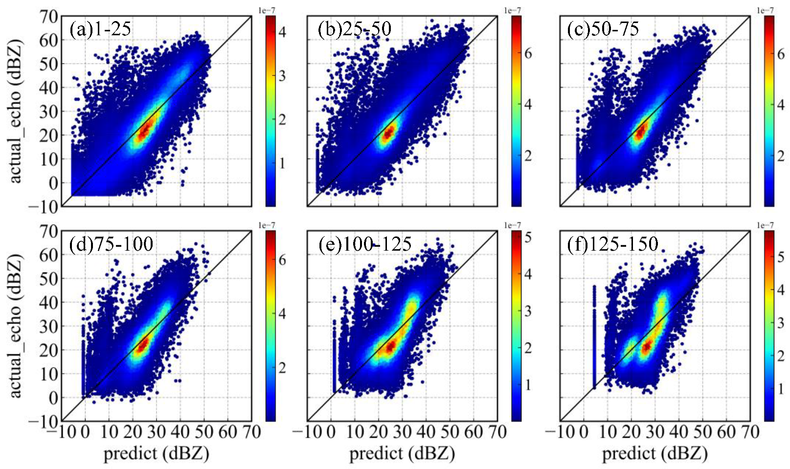
Figure 5 shows the six scatter plots of actual and predicted echo reflectivity with the test dataset of each section, where the loss function of MSE is used in the training process. The red line is a linear trend line of scattered points. The color mark represents the Gaussian kernel density estimation of the scatter point (Equations (10) and (11)). The larger the value is, the denser the scatter point.
f ^ s ( x ) = 1 n i = 1 n K s ( x x i ) = 1 n s i = 1 n K ( x x i s )
K ( x ) = 1 2 π exp ( 1 2 x 2 ) ,
where xi are sample points, s > 0 is a smoothing parameter called the bandwidth or window, K(x) is the kernel function, and it is a Gaussian curve. As shown in Figure 5, owing to the radar beam broadens with distance and altitude, the error in the long-distance section is larger than that in the close-distance section. In general, the six range section models perform well using the test set except for the section from 125 to 150 km, and most of the points are on the diagonal.
Table 2 lists the values of three evaluation indicators when models are compiled with the MSE as the loss function. The values of EVar in the models of sections from 1 to 75 km are above 0.85, and the others are all above 0.80. The MAEs are all 3–4 dB. For CCs, the values are all above 0.90 except for 0.88 in the section from 125 to 150 km. Therefore, all six echo-filling models using the MSE as the loss function have good performance and high accuracy.
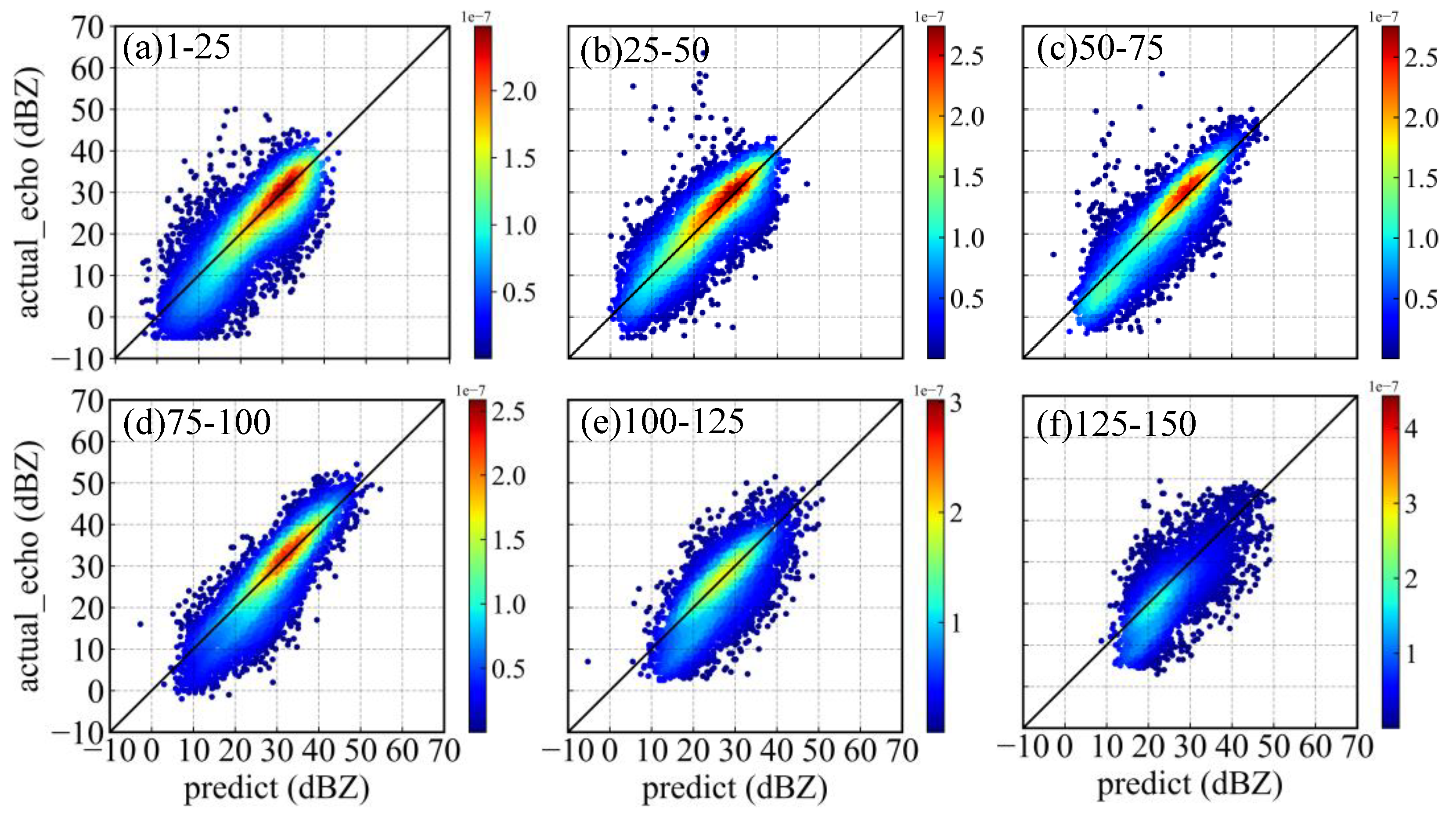
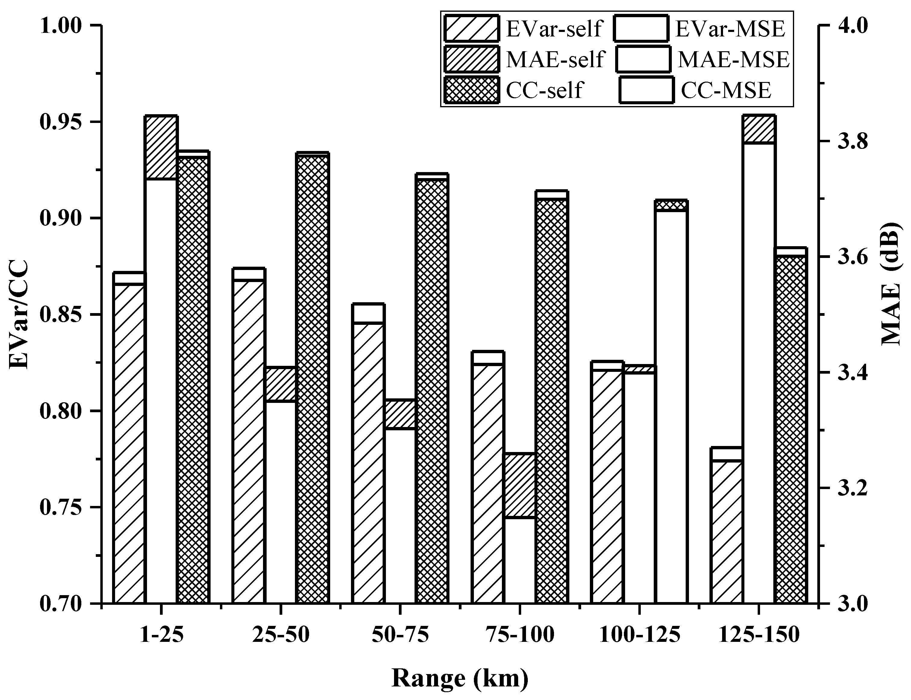
In Figure 5, the predicted strong echo is slightly lower than the measured value. Therefore, a self-defined loss function is proposed in Section 3.2 to improve the model fitting effect in the strong echo region. Figure 6 shows the scatter plot corresponding to Figure 5 but using the self-defined loss function, in which the strong echo points have been obviously improved. The values of the evaluation indicator are listed in Table 3, and a column chart of the comparison between Table 2 and Table 3 is shown in Figure 7. The performance of model compiled with the self-defined loss function is slightly worse than that with MSE, in which the average value of MAE increases by 0.0646 and EVar and CC decrease by 0.0067 and 0.0019, respectively, and it is mainly because the model with self-defined loss function highlights the strong echoes more but the proportion of strong echo is relatively small in the test dataset.

3.4. Comparing with Multivariable Linear Regression Models

In order to verify the advantages of deep learning algorithm, six multivariable linear regression models are established based on the same dataset as the EFnet but only N × 1 point are used as feature data instead of N × 3 × 3 points. Figure 8 shows the six scatter plots of actual and fitting echo reflectivity with the test dataset, it is obviously that the fitting effect with linear models are obviously worse than that with EFnet.

4. Case Study

Two volume scan data points observed with Nanjing CINRAD/SA radar are selected to verify the six models in different sections, which are trained and tested in Section 3. One of them demonstrated in Section 4.1 is dominated by the weak echoes at 0002 UTC on 2 July 2017, and the other in Section 4.2 is dominated by strong echoes at 1008 UTC on 3 July 2012. The outputs of the model are evaluated with the true value of reflectivity in the unblocked fan-shaped area, which is bounded by red lines in Figure 9 and Figure 13.

4.1. Weak Echoes-Dominated Case

The weak echoes-dominated volume data are arranged in the input format of the models and put into the models, and then, the predicted values of reflectivity in each section of 0.5° elevation are outputted by means of the model fitting. Figure 9 shows the plan position indicator (PPI) images of reflectivity at 0.5° elevation, where Figure 9a shows the raw observed image and Figure 9b,c shows prediction images by means of models that are compiled with the MSE and the self-defined loss function, respectively. Table 4 lists the evaluation results of models with two loss functions in the nonocclusion fan-shaped area, which are bounded by red lines in Figure 9.
As shown in Figure 9a, the case is dominated by weak echoes in which most echo intensity is less than 40 dBZ, and there is obvious terrain blockage in the third quadrant, which is marked with an ellipse of a red line in which the echoes are obviously weak and even disappear completely. Both the models with the MSE and the self-defined loss function can fill the echoes in the occlusion area well and effectively improve the echo structure to make it more accurate. Furthermore, the strong echoes area marked with the blue ellipse is more consistent between the raw data and the prediction with the self-defined loss function (Figure 9c) than with the MSE (Figure 9b). In other words, the model with the self-defined loss function is better than that with the MSE in fitting strong echoes.
In order to demonstrate the filling effect more clearly, three radial profiles at the blocked azimuth 215° in Figure 9 are shown in Figure 10, in which image (a) is the raw data and (b) and (c) are the corrected data with the MSE and the self-defined loss function, respectively. Both the models can correct the 0.5° occlusion well and make the vertical structure of cloud more complete. In the strong echoes area (red ellipse area), the filling echoes with the self-defined loss function are stronger than that with the MSE, which realizes the purpose of highlighting the strong echo.
The values of the model evaluation indicator for the case are listed in Table 4. The EVars of the two models are all above 0.85, the MAEs are approximately 4 dB, and the CCs are above 0.9 and even greater than 0.97 when using the self-defined loss function in the range from 25 to 50 km, which illustrates the effectiveness of the models quantitatively. Comparing the values in Table 4, the performance of model compiled with the self-defined loss function is slightly better than that with MSE, in which the average value of EVar increases by 0.0111, MAE and CC decrease by 0.2356 and 0.0087, respectively, and it is mainly because the proportion of strong echoes in the case is higher than that in the test dataset.
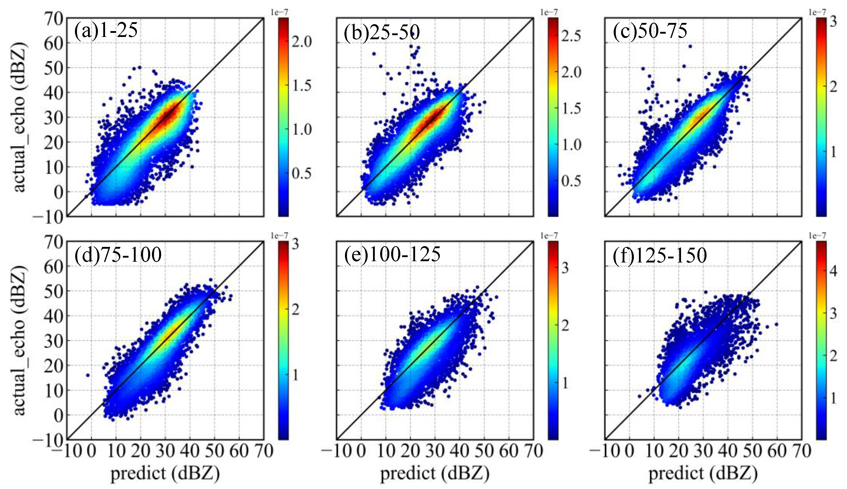
Figure 11 and Figure 12 show the scatter plots of the predicted and true reflectivity in the unblocked area in each section model compiled with the MSE and the self-defined loss function, respectively. Most of the points are near the diagonal, which illustrates that the models perform well.

4.2. Strong Echoes-Dominated Case

The strong echoes-dominated volume data are reshaped into the input format of each range section model, and then the values of reflectivity at 0.5° elevation are fitted by means of the models. Figure 13 shows the PPI images corresponding to Figure 9 except for the strong echoes. Similarly, Table 5 lists the evaluation indicators in the nonocclusion fan-shaped area bounded by red lines in Figure 13.
As shown in Figure 13, the shapes of the strong echo marked with the blue ellipse are basically consistent among the three PPIs, and the consistency between Figure 13a,c is better, which further illustrates that the self-defined loss function performs better on strong echo fitting. The points number of strong echo (>40 dBZ) in Figure 11 are counted. There are 1807 points (3.37%) in the actual PPI (Figure 13a), 1740 points (3.24%) in the PPI predicted with the MSE loss function model (Figure 13b) and 1841 points (3.43%) with the self-defined loss function model (Figure 13c), and the proportion of strong echo with the self-defined loss function is closer to that of raw observation.
In order to further verify the performance in strong echo area with the self-defined loss function, three radial profiles at the unblocked azimuth 48° in Figure 13 are plotted in Figure 14. As shown in the red ellipse area in the 0.5° elevation, comparing with the raw data (a), the strong echoes with the self-defined loss function (c) are more consistent than that with the MSE (b), which demonstrate that the model with the self-defined loss function is better than that with the MSE for fitting strong echoes.
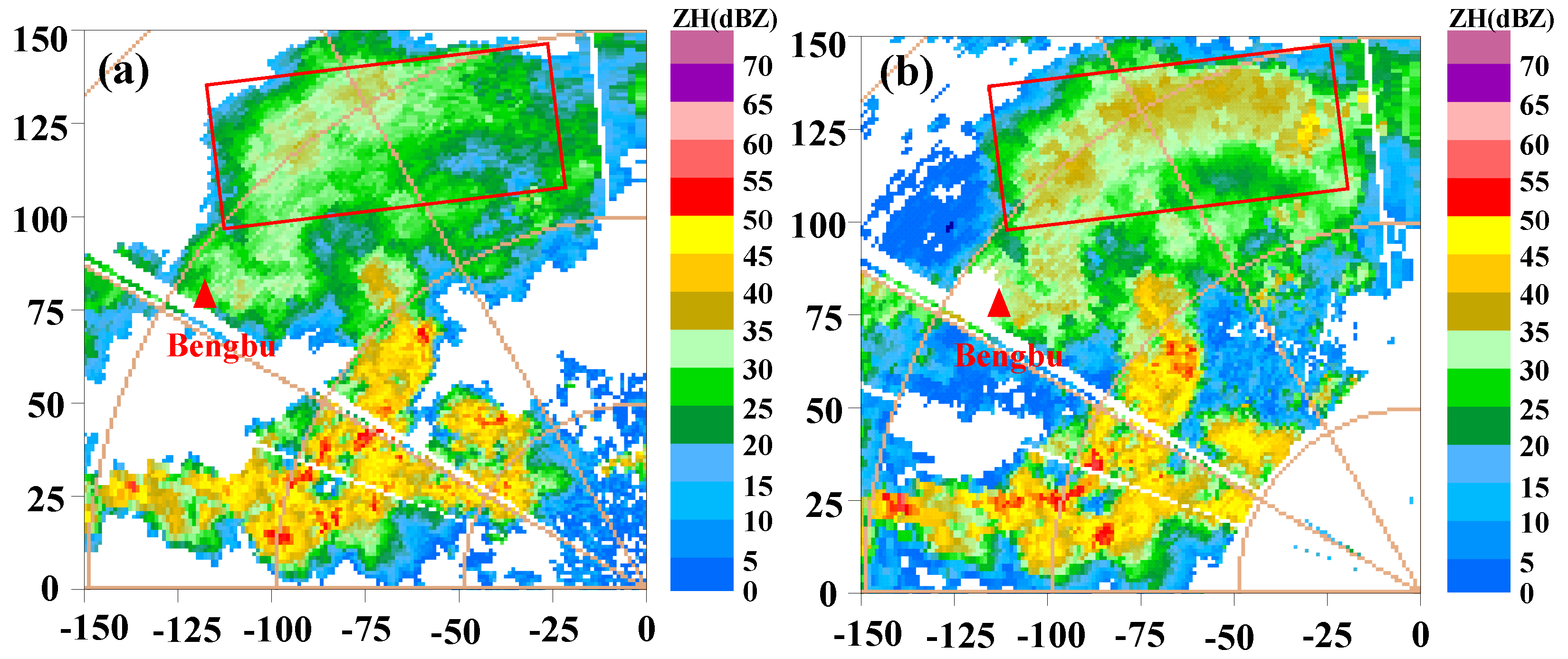
However, for weak echoes in the northwest direction beyond 100 km, the reflectivity estimated by the model is obviously stronger than that measured by the Nanjing radar. It is well known that the beam broadens and the echo intensity weakens with increasing distance from the radar. To compare filling effect, the reflectivity observed simultaneously with the Bengbu SA radar, which is located at Nanjing SA radar azimuth 303.5° and distance of 142.5 km (the red triangle in Figure 15), is interpolated to the gates of the Nanjing radar (Figure 15). It can be seen from the area marked with a rectangle of red lines in Figure 15 that the weak echoes observed with the Bengbu radar are obviously stronger than those observed with the Nanjing radar because of the distance. On the other hand, the echo predicted by the model is affected by the melting layer in far distance, so this strong echo area may be due to the insufficient melting layer data collected in the training dataset, which causes strong fitting results.
In Table 5, the EVars are all above 0.92 except for the models of the first range section from 1 to 25 km, the MAEs are less than 4.5 dB, and the CCs are greater than 0.96 except for the first section, which further verifies the effectiveness and stability of the deep learning algorithm applied to the echo correction. Comparing the values of the model evaluation indicator compiled with the self-defined loss function and MSE in Table 5, the average value of MAE decreases 0.1085 and EVar and CC increase 0.0023 and 0.0017, respectively, which suggests that the models with the self-defined loss function perform better.

5. Discussion

An EFnet based on a deep learning algorithm is used to fill and correct the radar reflectivity in the occlusion area at the 0.5° elevation angle, and a self-defined loss function is proposed to improve the model fitting in strong echoes. The training dataset is constructed with the data in unblocked areas in the Nanjing SA radar; six echo-filling models are built according to the range, and three indicators are utilized to evaluate the models. Whether from the subjective impression of the PPI images or from the quantitative analysis of the indicator tables, the results show that the low-level occlusion reflectivity has been corrected very well. This shows that deep learning has broad prospects in weather radar applications.
In the process of model training, data preprocessing, namely, data quality control and normalization, is a critical step. Other superparameter settings, such as the loss function, optimizer, number of hidden layers, nodes, and iteration epochs, also have a significant impact on the fitting effect to models, which needs to be adjusted and tested repeatedly.
Although the number of training datasets in this paper reaches approximately 200,000, it is still relatively small. In practical applications, the number of radar volume scan data can be greatly increased to make the training dataset reach more than several million, and the models will achieve a better fitting effect. In addition, more data of stable precipitation echo should be added into the training datasets to further improve the influence of melting layer.
When multiple elevation angles are blocked, the echo-filling model can be similarly established using deep learning. Compared with using only a single parameter of the reflectivity factor as input, the polarimetric parameters can be added as input features into the training data with the polarization upgrading of weather radar, which will effectively improve the effect of echo correction, and the polarization parameters can also be corrected by a similar deep learning network. In addition, some features, such as terrain, underlying surface information, and weather background, can also be applied to construct a multimodal model, which is a popular method for deep learning training at present. These means can achieve refined, intellectualized, and automatic echo correction for radar beam blockage.

Author Contributions

Conceptualization, X.Y. and Z.H.; methodology, Z.H.; software, B.L.; validation, J.Z., B.L. and Y.Z.; formal analysis, J.Z.; investigation, B.L.; resources, J.Z.; data curation, Y.Z.; writing—original draft preparation, X.Y.; writing—review and editing, X.Y. and Z.H.; visualization, X.Y.; supervision, Z.H.; project administration, Z.H.; funding acquisition, Z.H. All authors have read and agreed to the published version of the manuscript.

Funding

This research was funded by the “Key-Area Research and Development Program of Guangdong Province (2020B1111200001)”, the “Key project of monitoring, early warning and prevention of major natural disasters of China (2019YFC1510304)”, and the “Scientific Research Projects of Weather Modification in Northwest China (RYSY201905)”.

Data Availability Statement

The data presented in this study are available on request from the corresponding author.

Acknowledgments

The authors would like to sincerely thanks Fen Xu of Nanjing Joint Institute for Atmospheric Sciences for providing technical guidance.

Conflicts of Interest

The authors declare no conflict of interest. The funders had no role in the design of the study; in the collection, analyses, or interpretation of data; in the writing of the manuscript; or in the decision to publish the results.

References

  1. Yu, X.D.; Yao, X.P.; Xiong, T.N.; Zhou, X.G.; Wu, H.; Deng, B.S.; Song, Y. Principle and Application of Doppler Weather Radar; China Meteorological Press: Beijing, China, 2006; pp. 63–72. [Google Scholar]
  2. Westrick, K.J.; Mass, C.F.; Colle, B.A. The Limitations of the WSR-88D Radar Network for Quantitative Precipitation Measurement over the Coastal Western United States. Bull. Amer. Meteor. Soc. 1999, 80, 2289–2298. [Google Scholar] [CrossRef]
  3. Germann, U.; Joss, J. Operational Measurement of Precipitation in Mountainous Terrain; Springer: Berlin/Heidelberg, Germany, 2004; pp. 52–77. [Google Scholar]
  4. Battan, L.J. Radar Observation of the Atmosphere; The University of Chicago Press: Chicago, IL, USA, 1973. [Google Scholar]
  5. Lang, T.J.; Nesbitt, S.W.; Carey, L.D. On the Correction of Partial Beam Blockage in Polarimetric Radar Data. J. Atmos. Ocean. Technol. 2009, 26, 943–957. [Google Scholar] [CrossRef] [Green Version]
  6. Luo, L.; Jing, G.F.; Guo, J.; You, Y. Frequency of the “Cross Points” of Rayleigh Wave Dispersion Curves in Multi-layered Medium with Low Velocity Layer. Sci. Technol. Eng. 2016, 16, 12–19. (In Chinese) [Google Scholar]
  7. Lee, J.; Jung, S.H.; Kim, H.L.; Lee, S.K. Improved Rainfall Estimation Based on Corrected Radar Reflectivity in Partial Beam Blockage Area of S-band Dual-Polarization Radar. Korean Meteorol. Soc. 2017, 27, 467–481. [Google Scholar]
  8. Zhang, Y.P.; Liu, J.; Xia, W.M.; Gu, S.S. The Calculation of Beam Blockage Coefficients in Estimating Regional Precipitation with Radar. J. Nanjing Inst. Meteorol. 2002, 25, 67–74. (In Chinese) [Google Scholar]
  9. Yang, H.P.; Zhang, P.Y.; Cheng, M.H.; Li, B.; Xiong, Y.; Gao, Y.C.; Chen, D.R. The Valid Mosaic Data Region of the CINRAD Network. J. Appl. Meteorol. Sci. 2009, 20, 47–55. (In Chinese) [Google Scholar]
  10. Shakti, P.C.; Maki, M.; Shimizu, S.; Maesaka, T.; Kim, D.-S.; Lee, D.-I.; Iida, H. Correction of Reflectivity in the Presence of Partial Beam Blockage over a Mountainous Region Using X-Band Dual Polarization Radar. J. Hydrometeorol. 2013, 14, 744–764. [Google Scholar]
  11. Gou, Y.B.; Liu, L.P.; Li, R.Y.; Du, M.Y.; Duan, Y.P. Radar Partial Shielding Region Identification Algorithm Based on the Probability Characteristics of Radar Echoes. Plateau Meteorol. 2015, 34, 556–567. (In Chinese) [Google Scholar]
  12. Huang, X.Y.; Ma, L.; Yang, M.; Yin, J.N.; Liu, Y.F. Recognition and correction of beam blockage of weather radar based on spatial correlation. Sci. Meteorol. Sinica 2019, 39, 532–539. (In Chinese) [Google Scholar]
  13. Germann, U.; Galli, G.; Boscacci, M.; Bolliger, M. Radar precipitation measurement in a mountainous region. Quart. J. Roy. Meteorol. Soc. 2006, 132, 1669–1692. [Google Scholar] [CrossRef]
  14. Tabary, P. The New French Operational Radar Rainfall Product. Part I: Methodology. Weather Forecast. 2007, 22, 393–408. [Google Scholar] [CrossRef]
  15. Germann, U.; Joss, J. Mesobeta Profiles to Extrapolate Radar Precipitation Measurements above the Alps to the Ground Level. J. Appl. Meteorol. 2002, 41, 542–557. [Google Scholar] [CrossRef]
  16. Yang, F.; Gu, S.S.; Huang, X.Y.; Sun, Q.; Wu, L.L.; Xia, W.M. Determination of Vertical Profiles of Reflectivity for Estimation of Stratiform Cloud Precipitation in Ground Clutter Areas. J. Nanjing Inst. Meteorol. 2009, 32, 145–150. (In Chinese) [Google Scholar]
  17. Andrieu, H.; Creutin, J.D.; Delrieu, G.; Faure, D. Use of a weather radar for the hydrology of a mountainous area. Part I: Radar measurement interpretation. J. Hydrol. 1997, 193, 1–25. [Google Scholar] [CrossRef]
  18. Creutin, J.D.; Andrieu, H.; Faure, D. Use of a weather radar for the hydrology of a mountainous area. Part II: Radar measurement validation. J. Hydrol. 1997, 193, 26–44. [Google Scholar] [CrossRef]
  19. Yang, L.; Liu, L.P.; Wang, H.Y. Filling-up of Occultation Regions Using Vertical Profile of Reflectivity Factor. Meteor. Sci. Technol. 2015, 43, 788–793. (In Chinese) [Google Scholar]
  20. Tan, C.; Feng, X.; Long, J.; Geng, L. FORECAST-CLSTM: A New Convolutional LSTM Network for Cloudage Nowcasting. In Proceedings of the 2018 IEEE Visual Communications and Image Processing (VCIP), Taichung, Taiwan, 9–12 December 2018; pp. 1–4. [Google Scholar]
  21. Gorooh, V.A.; Kalia, S.; Nguyen, P.; Hsu, K.; Sorooshian, S.; Ganguly, S.; Nemani, R. Deep Neural Network Cloud-Type Classification (DeepCTC) Model and Its Application in Evaluating PERSIANN-CCS. Remote Sens. 2020, 12, 316. [Google Scholar] [CrossRef] [Green Version]
  22. Lee, J.; In, J.; Cha, D.H.; Park, H.; Sim, S. Tropical Cyclone Intensity Estimation Using Multi-Dimensional Convolutional Neural Networks from Geostationary Satellite Data. Remote Sens. 2020, 12, 108. [Google Scholar] [CrossRef] [Green Version]
  23. Fabry, F. Radar Meteorology—Principles and Practice; Cambridge University Press: Cambridge, UK, 2015; p. 272. [Google Scholar]
  24. Shi, X.; Chen, Z.; Wang, H.; Yeung, D.Y.; Wong, W.K.; Woo, W.C. Convolutional LSTM network: A machine learning approach for precipitation nowcasting. In Proceedings of the 28th International Conference on Neural Information Processing Systems (NeurIPS), Montreal, QC, Canada, 7–12 December 2015; pp. 802–810. [Google Scholar]
  25. Zhou, K.H.; Zheng, Y.G.; Li, B.; Dong, W.; Zhang, X.L. Forecasting different types of convective weather: A deep learning approach. J. Meteorol. Res. 2019, 33, 797–809. [Google Scholar] [CrossRef]
  26. Tran, Q.K.; Song, S.K. Multi-Channel Weather Radar Echo Extrapolation with Convolutional Recurrent Neural Networks. Remote Sens. 2019, 11, 2303. [Google Scholar] [CrossRef] [Green Version]
  27. Wei, C.C.; Hsieh, P.Y. Estimation of Hourly Rainfall during Typhoons Using Radar Mosaic-Based Convolutional Neural Networks. Remote Sens. 2020, 12, 896. [Google Scholar] [CrossRef] [Green Version]
  28. Bouget, V.; Béréziat, D.; Brajard, J.; Charantonis, A.; Filoche, A. Fusion of Rain Radar Images and Wind Forecasts in a Deep Learning Model Applied to Rain Nowcasting. Remote Sens. 2021, 13, 246. [Google Scholar] [CrossRef]
  29. Liu, L.P.; Wu, L.L.; Yang, Y.M. Development of Fuzzy-logical Two-step Ground Clutter Detection Algorithm. Acta Meteorol. Sinica. 2007, 65, 252–260. (In Chinese) [Google Scholar]
  30. Li, F.; Liu, L.P.; Wang, H.Y.; Jiang, Y. Identification of Non-precipitation Meteorological Echoes with Doppler Weather Radar. J. Appl. Meteor. Sci. 2012, 23, 147–158. (In Chinese) [Google Scholar]
  31. Wen, H.; Liu, L.P.; Zhang, Y. Improvements of ground clutter identification algorithm for Doppler Weather Radar. Plateau Meteor. 2017, 36, 736–746. (In Chinese) [Google Scholar]
  32. Zhang, P.C.; Dai, T.P.; Du, B.Y. Radar Meteorology; China Meteorological Press: Beijing, China, 2001; pp. 100–103. [Google Scholar]
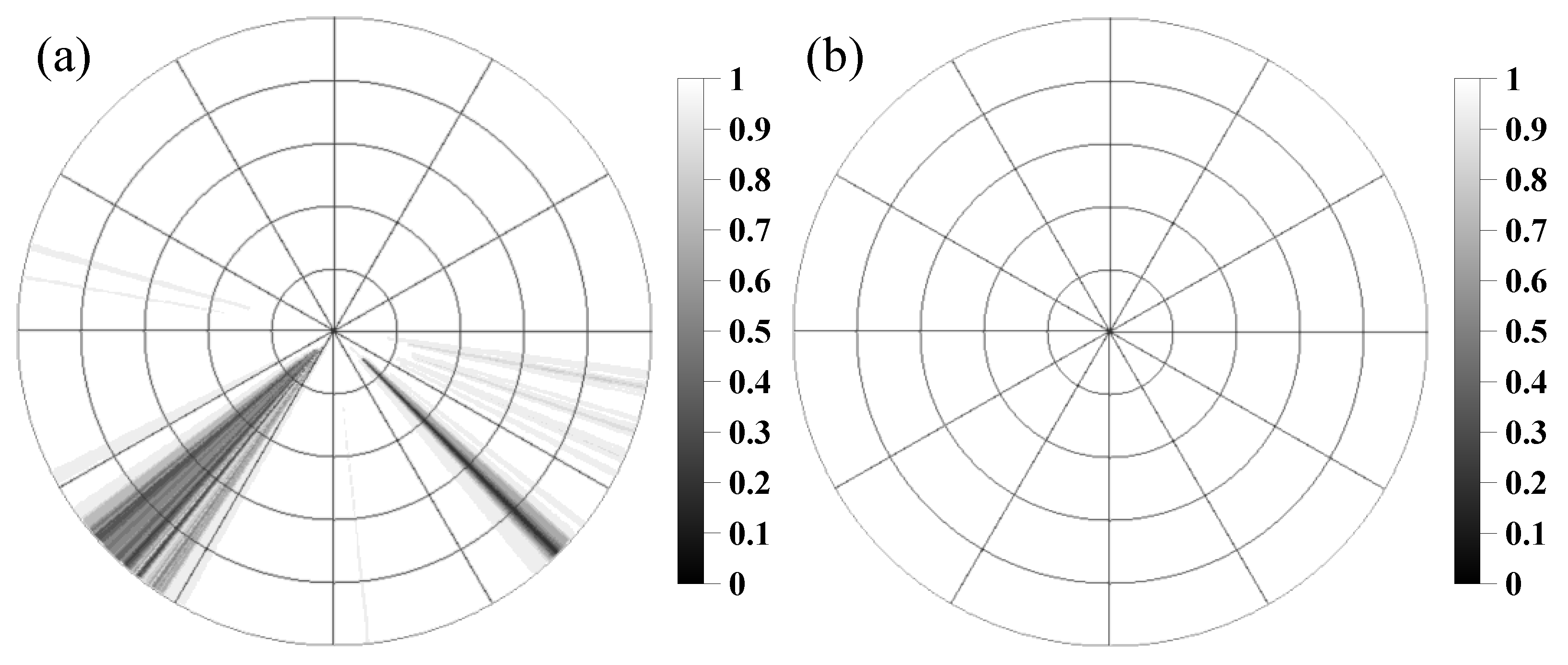
Figure 1. Transmittance of the Nanjing S-band new-generation Doppler weather radar (SA) at the elevation angle of 0.5° (a) and 1.5° (b).
Remotesensing 13 01779 g001
Figure 2. Sketch map of radar beam propagation in a standard atmosphere. The lower right corner shows the 3 × 3 features, and the black point is the corresponding location of the label at the bottom.
Remotesensing 13 01779 g002
Figure 3. Echo-filling network (EFnet) architecture.
Remotesensing 13 01779 g003
Figure 4. Modeling flow chart.
Remotesensing 13 01779 g004
Figure 5. Scatter plots of the actual and predicted echo reflectivity with the test dataset of each section, where the loss function of mean square error (MSE) is used during the training process. In which the red line denotes a linear trend line of scattered points, and color mark represents the Gaussian kernel density estimation of the scatter point.
Remotesensing 13 01779 g005
Figure 6. Scatter plot corresponding to Figure 5 but using the self-defined loss function.
Remotesensing 13 01779 g006
Figure 7. Column chart of comparison between Table 2 and Table 3.
Remotesensing 13 01779 g007
Figure 8. The six scatter plots of actual and fitting echo reflectivity with the test dataset of each section using the multivariable linear regression models.
Remotesensing 13 01779 g008
Figure 9. Plan position indicator (PPI) images of reflectivity at 0.5° elevation: (a) is the raw observed image and (b,c) are prediction images by means of models compiled with the MSE and the self-defined loss function, respectively, in which the distance circle is 25 km (the same below), the red ellipse is the serious occlusion area, and the blue ellipse is one of the strong echo areas.
Remotesensing 13 01779 g009
Figure 10. Radial profiles at the blocked azimuth 215° in Figure 9, in which image (a) is the raw data and (b,c) are the corrected data with the MSE and the self-defined loss function, respectively; the red ellipse areas are for comparison.
Remotesensing 13 01779 g010
Figure 11. Scatter plots between true reflectivity and the model prediction in each section using the MSE loss function in this case with weak echoes-dominated volume data.
Remotesensing 13 01779 g011
Figure 12. Scatter plots corresponding to Figure 11 but using the self-defined loss function.
Remotesensing 13 01779 g012
Figure 13. PPI images of reflectivity at 0.5° elevation: (a) is the raw observed image and (b,c) are prediction images by means of models compiled with the MSE and the self-defined loss function, respectively, in which the blue ellipse mark the strong echo areas.
Remotesensing 13 01779 g013
Figure 14. Radial profiles at the unblocked azimuth 48° in Figure 13, in which image (a) is the raw data and (b,c) are the filling data with the MSE and the self-defined loss function, respectively; the red ellipse areas are for comparison.
Remotesensing 13 01779 g014
Figure 15. The weak echoes area in Figure 13 observed with the Nanjing radar (a) and interpolated with the Bengbu radar (b), where the red triangle is the location of the Bengbu radar.
Remotesensing 13 01779 g015
Table 1. The data size in the six sections.
Range (km)1–2525–5050–7575–100100–125125–150
Using elevation layer number765432
Data size (group)171,887190,182199,830185,808201,990182,676
Training set size (80%)137,510152,146159,864148,646161,592146,141
Test set size (20%)34,37738,03639,96637,16240,39836,535
Table 2. Values of the evaluation indicator with the mean square error (MSE) as the loss function.
Range (km)1–2525–5050–7575–100100–125125–150
EVar0.87170.87390.85550.83090.82560.7809
MAE3.73403.35013.30283.14893.39893.7964
CC0.93460.93400.92300.91420.90390.8846
Table 3. Values of evaluation indicator with the self-defined loss function.
Range (km)1–2525–5050–7575–100100–125125–150
EVar0.86560.86770.84550.82410.82100.7740
MAE3.84353.40843.35203.25923.41123.8445
CC0.93140.93210.91990.90970.90920.8802
Table 4. Values of the evaluation indicator in the nonocclusion area of Figure 9 with weak echoes-dominated volume data.
Range (km)1–2525–5050–7575–100100–125125–150
MSE loss functionEVar0.91560.94810.86520.83730.88090.9029
MAE4.28953.10313.20993.92773.92774.3006
CC0.96100.97350.93780.94150.94150.9505
Self-defined loss functionEVar0.92430.94860.86850.85620.86960.9496
MAE4.05802.95733.25462.94473.91764.2122
CC0.96350.97490.93410.93750.94230.9012
Table 5. Values of the evaluation indicator in the nonocclusion area of Figure 13 with strong echoes-dominated volume data.
Range (km)1–2525–5050–7575–100100–125125–150
MSE loss functionEVar0.87090.92840.94970.94880.94880.9354
MAE4.47454.49303.86824.39503.98594.4552
CC0.93330.96360.97450.97460.97430.9671
Self-defined loss functionEVar0.87630.93010.95350.95350.94830.9342
MAE4.36814.50813.63624.12023.88354.5047
CC0.93740.96470.97670.97650.97560.9666
Publisher’s Note: MDPI stays neutral with regard to jurisdictional claims in published maps and institutional affiliations.