Self-Matching CAM: A Novel Accurate Visual Explanation of CNNs for SAR Image Interpretation

Abstract

Synthetic aperture radar (SAR) image interpretation has long been an important but challenging task in SAR imaging processing. Generally, SAR image interpretation comprises complex procedures including filtering, feature extraction, image segmentation, and target recognition, which greatly reduce the efficiency of data processing. In an era of deep learning, numerous automatic target recognition methods have been proposed based on convolutional neural networks (CNNs) due to their strong capabilities for data abstraction and mining. In contrast to general methods, CNNs own an end-to-end structure where complex data preprocessing is not needed, thus the efficiency can be improved dramatically once a CNN is well trained. However, the recognition mechanism of a CNN is unclear, which hinders its application in many scenarios. In this paper, Self-Matching class activation mapping (CAM) is proposed to visualize what a CNN learns from SAR images to make a decision. Self-Matching CAM assigns a pixel-wise weight matrix to feature maps of different channels by matching them with the input SAR image. By using Self-Matching CAM, the detailed information of the target can be well preserved in an accurate visual explanation heatmap of a CNN for SAR image interpretation. Numerous experiments on a benchmark dataset (MSTAR) verify the validity of Self-Matching CAM.

1. Introduction

Synthetic aperture radar (SAR) can produce high-resolution radar images in various extreme weather conditions, such as precipitation, dust, mist, etc., which makes it widely applied in many fields, like topographic mapping, urban planning, traffic monitoring, electronic reconnaissance, etc. [1,2,3,4]. Nowadays, it is increasingly important to obtain high-performance SAR images and clear interpretation of SAR images. With the application of various advanced SARs and numerous excellent imaging algorithms, there have been a larger number of high-performance SAR images, whereas, the interpretation of these images develops far behind forging them. SAR image interpretation usually includes image segmentation, target detection, and recognition, among which target recognition is deemed the most challenging task [1,5,6]. In traditional target recognition, SAR images first need a series of preprocessing operations, such as filtering, edge detection, region of interest (ROI) extraction, and feature extraction, and then a classifier like a support vector machine (SVM), perceptron, decision tree, K-nearest neighbor (KNN), etc., is utilized to categorize them to a corresponding class [7].

Note that traditional target recognition technology is composed of multiple individual steps [8,9,10]. Such complex procedures will reduce processing efficiency and make it difficult to realize real-time applications. In contrast, deep learning algorithms can allay the aforementioned limitations greatly because deep networks own an end-to-end structure without complex preprocessing operations [11,12]. Such an end-to-end structure can automatically learn the most discriminative information on a specific target from SAR images from low-dimension space to further high-dimension space for classification. In this case, the efficiency will be enhanced dramatically as long as the network is well trained. The convolutional neural network (CNN) is one of the most successful models in various computer vision fields [2,13,14,15]. The key to its superiority lies in the way it uses local connections and shared weights. Such operations can not only reduce the number of neurons but also preserve local characteristics of the input images. In SAR image target recognition, CNN has realized numerous remarkable achievements. Ref. [1] used CNN to implement target recognition on MSTAR data and obtained better accuracy than a SVM. Ref. [16] proposed an automatic SAR target recognition method combined with a CNN and a SVM. Ref. [17] designed a gradually distilled CNN with a small structure and high calculation efficiency for SAR target recognition. Ref. [18] designed a large-margin softmax batch-normalization CNN (LM-NB-CMM) for SAR target recognition of ground vehicles, which possessed better generalization performance, and achieved higher recognition accuracy and convergence speed compared with traditional CNN structures.

Although the aforementioned CNN-based methods can achieve high recognition performance and calculation efficiency, a CNN is usually used as a “black box” whose innate recognition mechanism still lacks analytical or mathematical explanation [19,20]. In this case, the reliability of recognition results is less convincing than traditional target recognition methods, which is sometimes fatal and unacceptable, particularly in some special scenarios [21,22]. To obtain a better explanation of a CNN’s mechanism, a number of methods have been proposed to visualize the internal representations learned by CNNs in the recent half-decade [23,24,25,26,27,28]. These methods are developed to highlight the regions of an image that are responsible for CNN decisions, which can be further divided into three categories: perturbation-based, propagation-based, and class activation mapping (CAM) methods. Perturbation-based methods occlude some patches of an image with black squares and detect whether there is an obvious drop of class score, then a heatmap can be produced according to the change of class score. Propagation-based methods are faster. They use gradients to visualize relevant regions for a given class, whereas the generated heatmaps are usually noisy. In contrast, CAM methods visualize CNN decisions using feature maps of deep layers, which can provide a mathematically explicable heatmap with some extent. In this paper, a CAM method is adopted as the visualization tool rather than perturbation algorithms and propagation algorithms due to the following. (1) CAM correlates the feature maps in a CNN’s hidden layer with heatmap generation while perturbation algorithms only occlude or conserve some patches in input images. (2) Although propagation algorithms can avoid gradient calculation to run faster, they are difficult to be applied to CNNs since a rather complicated correspondence exists between weights and elements in feature maps of a certain convolutional layer. Recently, increasing attention has been drawn to CAM, and numerous novel CAM methods have been proposed, such as Grad-CAM [24], Grad-CAM++ [25], XGrad-CAM [26], Ablation-CAM [27], Score-CAM [28], etc. However, these CAM methods show restrained effects on SAR image target recognition tasks because the SAR images are different from ordinary optical images including imaging mechanisms and wavelength range. In this paper, a Self-Matching CAM is proposed to highlight a more precise region of the target for classification than the above CAM methods. Numerous experimental results are conducted on a benchmark dataset (MSTAR) to verify the validity of the Self-Matching CAM.

The remainder of this paper is organized as follows. For a better understanding of CAM, Section 2 reviews several state-of-the-art CAM algorithms. Section 3 introduces the Self-Matching CAM in detail. Section 4 provides numerous experimental results from various perspectives to compare the performance of Self-Matching CAM with other available CAM methods. Section 5 discusses the experimental results and clarifies some confusion. Finally, Section 6 concludes this paper and discusses future work.

2. Related Work

CAM was first proposed in [23] by Zhou, B.L., Khosla, A., et al. CAM is specially designed for CNNs with only global average pooling (GAP) in the last convolutional layer. This means that each feature map in the last convolutional layer will be compressed to a single pixel value and then connected to neurons in fully connected layers. In this case, the final classification score $S_c$ for a specific class c can be formulated as a linear combination of feature maps $A^k$ of the convolutional layer (without regard to the activation function):

$$\begin{array}{c}\hfill S_c=\underset{k}{\mathsf{\Sigma }}{\omega }_k^c\underset{i}{\mathsf{\Sigma }}\underset{j}{\mathsf{\Sigma }}{A}_{ij}^k\end{array}$$

(1)

where ${\omega }_k^c$ is the weight corresponding to class c for the unit that is pooled from the feature map in the k-th channel, and $A_{ij}^k$ refers to the value of the k-th feature map in coordinates (i,j). The spatial element of the CAM heatmap for class c is defined by

$$\begin{array}{c}\hfill H_{ij}^{CAM}=\underset{k}{\mathsf{\Sigma }}{\omega }_k^c{A}_{ij}^k\end{array}$$

(2)

where $H_{ij}^{CAM}$ denotes the elements of the heatmap in coordinates (i,j).

While CAM is very straightforward since the weights naturally represent the importance of corresponding feature maps for classification, the limitation of CAM is apparent: it is unsuitable for CNNs without GAP in the last convolutional layer. To avoid changing the CNN structure, numerous modified CAM methods have been proposed for CNNs with any pooling rules. They can mainly be categorized into gradient-based methods and gradient-free methods.

In the following, we will review three gradient-based CAM methods (Grad-CAM, Grad-CAM++, and XGrad-CAM) and two gradient-free CAM methods (Ablation-CAM and Score-CAM). At the end of this section, we will discuss some challenges with which CAM methods are confronted in SAR image processing.

2.1. Gradient-Based Methods

Equation (2) gives the general definition of CAM. Different definitions of ${\omega }_k^c$ lead to different CAM methods. Gradient-based methods formulate weights ${\omega }_k^c$ with the partial derivative of $S_c$ with respect to $A^k$. To avoid confusion, in the following, we use ${\alpha }^{ck}$ to replace ${\omega }_k^c$ (${\omega }_k^c$ represents the weights between the GAP layer and the fully connected layer, while ${\alpha }^{ck}$ only denotes the coefficients of a linear combination of feature maps). Grad-CAM is one of the most well-known and widely used gradient-based methods [24]. It defines the weights ${\alpha }^{ck\_grad}$ as:

$$\begin{array}{c}\hfill {\alpha }^{ck\_grad}=\frac{1}{Z}\underset{i}{\mathsf{\Sigma }}\underset{j}{\mathsf{\Sigma }}\frac{\partial S_c}{\partial A_{ij}^k}\end{array}$$

(3)

where Z is the number of pixels in the feature map. Therefore, Grad-CAM can be applied to any deep CNN without any modification of network structure as long as $S_c$ is a differentiable function of feature maps $A^k$. Grad-CAM is applicable to any CNN structures, which greatly overcomes the limitations of CAM. However, Grad-CAM is still not a panacea due to the following: (1) it does not explain clearly why it uses the average of gradients to weight each feature maps; (2) an unweighted average of the partial derivatives usually leads to an excessive highlighted region covering the target in the SAR image overlay.

To highlight the target in the heatmap precisely, ref. [25] proposed Grad-CAM++ introducing second and third partial derivative form weights ${\alpha }^{ck\_++}$ formulated as:

$$\begin{array}{c}\hfill {\alpha }^{ck\_++}=\underset{i}{\mathsf{\Sigma }}\underset{j}{\mathsf{\Sigma }}[\frac{\frac{{\partial }^2{S}_c}{{(\partial A_{ij}^k)}^2}}{2\frac{{\partial }^2{S}_c}{{(\partial A_{ij}^k)}^2}+\underset{x}{\mathsf{\Sigma }}\underset{y}{\mathsf{\Sigma }}{A}_{xy}^k\{\frac{{\partial }^3{S}_c}{{(\partial A_{ij}^k)}^3}\}}]·\frac{\partial S_c}{\partial A_{ij}^k}\end{array}$$

(4)

where ${\alpha }^{ck\_++}$ denotes the element of weights to the k-th feature map for class c in coordinates (i,j). It is evident that, if $\forall i$,j, ${\alpha }^{ck\_++}=\frac{1}{Z}$, Grad-CAM++ degenerates into Grad-CAM. In Grad-CAM++, a weighted partial derivative replaces the unweighted average of the gradient, thus the highlighted region in the heatmaps is usually narrower than Grad-CAM.

However, Grad-CAM++ still does not explain clearly why such a weighted partial derivative works in locating the target precisely. Ref. [26] proposed an axiom-based CAM (XGrad-CAM) with a clear mathematical explanation to achieve better visualization of the CNN’s decision than Grad-CAM++. XGrad-CAM formulates ${\alpha }^{ck}$ by introducing two axioms: sensitivity and conservation. They are self-evident properties that visualization methods are supposed to satisfy [29], defined as follows:

$$\begin{array}{cc}\hfill & \mathrm{Sensitivity}:S_c(A)-S_c(A\backslash A^k)=\underset{i}{\mathsf{\Sigma }}\underset{j}{\mathsf{\Sigma }}{\alpha }^{ck}{A}_{ij}^k\hfill \end{array}$$

(5)

$$\begin{array}{cc}\hfill & \mathrm{Conservation}:S_c(A)=\underset{i}{\mathsf{\Sigma }}\underset{j}{\mathsf{\Sigma }}(\underset{k}{\mathsf{\Sigma }}{\alpha }^{ck}{A}_{ij}^k)\hfill \end{array}$$

(6)

where $S_c(A\backslash A^k)$ is the score of class c when the k-th feature map in the target layer has been replaced by zero. The meaning of sensitivity is straightforward in that if a large drop of class score emerges when the k-th feature map is removed, then this feature map should be assigned a high weight. Conservation is used to ensure that the class score is mainly dominated by the feature maps rather than other factors. To meet these two axioms, ref. [26] transforms this into a minimization problem of $\varphi ({\alpha }^{ck})$ as below:

$$\begin{array}{c}\hfill \varphi ({\alpha }^{ck})=\underset{k}{\mathsf{\Sigma }}|S_c(A)-S_c(A\backslash A^k)-\underset{i}{\mathsf{\Sigma }}\underset{j}{\mathsf{\Sigma }}{\alpha }^{ck}{A}_{ij}^k|+|S_c(A)-\underset{i}{\mathsf{\Sigma }}\underset{j}{\mathsf{\Sigma }}(\underset{k}{\mathsf{\Sigma }}{\alpha }^{ck}{A}_{ij}^k)|.\end{array}$$

(7)

Ref. [26] proves that for a convolutional layer in a ReLU-CNN, which only has ReLU activation functions as its non-linearities, the class score is equivalent to the sum of the element-wise product between feature maps and gradient maps of the target layer, written as:

$$\begin{array}{c}\hfill S_c(A)=\underset{k}{\mathsf{\Sigma }}\underset{i}{\mathsf{\Sigma }}\underset{j}{\mathsf{\Sigma }}(\frac{\partial S_c(A)}{\partial A_{ij}^k}{A}_{ij}^k)+\underset{t=l+1}{\overset{L}{\mathsf{\Sigma }}}\underset{n}{\mathsf{\Sigma }}\frac{\partial S_c(A)}{\partial u_n^t}{b}_n^t\end{array}$$

(8)

where l is the order of the last convolutional layer, L is the number of layers in the CNN, $u_n^t$ denotes the n-th neuron in the t-th layer ($t>l$), and $b_n^t$ is the bias corresponding to $u_n^t$. Substituting Equation (8) into Equation (7), we can rewrite $\varphi ({\alpha }^{ck})$ as:

$$\begin{array}{c}\hfill \varphi ({\alpha }^{ck})=\underset{k}{\mathsf{\Sigma }}|\underset{i}{\mathsf{\Sigma }}\underset{j}{\mathsf{\Sigma }}(\frac{\partial S_c(F)}{\partial A_{ij}^k}-{\alpha }^{ck}{A}_{ij}^k)+\xi (A;k)|+\\ \hfill |\underset{k}{\mathsf{\Sigma }}\underset{i}{\mathsf{\Sigma }}\underset{j}{\mathsf{\Sigma }}(\frac{\partial S_c(F)}{\partial A_{ij}^k}-{\alpha }^{ck}{A}_{ij}^k))+\underset{t=l+1}{\overset{L}{\mathsf{\Sigma }}}(\underset{n}{\mathsf{\Sigma }}\frac{\partial S_c(A)}{\partial u_n^t})|.\end{array}$$

(9)

where $\xi (A;k)=\underset{k^{{}^{\prime }},k^{{}^{\prime }}\ne k}{\mathsf{\Sigma }}\underset{i}{\mathsf{\Sigma }}\underset{j}{\mathsf{\Sigma }}(\frac{\partial S_c(A)}{\partial A_{ij}^k}{A}_{ij}^{k^{{}^{\prime }}}-\frac{\partial S_c(A\backslash A^k)}{\partial A_{ij}^k}{A}_{ij}^{k^{{}^{\prime }}})$ and $\underset{t=l+1}{\overset{L}{\mathsf{\Sigma }}}\underset{n}{\mathsf{\Sigma }}\frac{\partial S_c(A)}{\partial u_n^t}{b}_n^t$ are two considerably small terms that can be ignored. Without considering these two terms, we can calculate an approximate optimal solution ${\alpha }^{ck}$ to Equation (7):

$$\begin{array}{c}\hfill {\alpha }^{ck\_Xgrad}=\underset{i}{\mathsf{\Sigma }}\underset{j}{\mathsf{\Sigma }}(\frac{A_{ij}^k}{\underset{i}{\mathsf{\Sigma }}\underset{j}{\mathsf{\Sigma }}{A}_{ij}^k}\frac{\partial S_c(A)}{\partial A_{ij}^k}).\end{array}$$

(10)

2.2. Gradient-Free Methods

Gradient-free methods abandon forming weights with partial derivatives, because advocates of gradient-free methods think that it is easy to find samples with false confidence by using gradients, i.e., some feature maps with high gradients contribute less to the network classification. The way that gradient-free methods acquire weights is more intuitive and straightforward. Here we review two famous methods: Ablation-CAM and Score-CAM.

Ablation-CAM was proposed in [27], where an ablation study was used to determine the importance of each pixel in the feature map. Specifically, Ablation-CAM calculates the contribution of each feature map for classification by removing a specific feature map while retaining the rest. In Ablation-CAM, the slope is used to describe the effect of removing the k-th feature map, defined as:

$$\begin{array}{c}\hfill slope=\frac{S_c(A)-S_c(A\backslash A^k)}{\parallel A^k\parallel }\end{array}$$

(11)

where $\parallel A^k\parallel$ is the two-norm of $A^k$. Since calculation of the $slope$ is time-consuming, ref. [27] proposed an approximate solution as:

$$\begin{array}{c}\hfill {\alpha }^{ck\_Ablation}=\frac{S_c(A)-S_c(A\backslash A^k)}{S_c(A)}.\end{array}$$

(12)

The effect of Ablation-CAM is better than Grad-CAM and Grad-CAM++ on optical images; however, this method is quite time-consuming since it has to run forward propagation hundreds of times per image. Ref. [28] proposed Score-CAM by introducing the increase of confidence (CIC) as a weight for a feature map, defined as:

$$\begin{array}{cc}\hfill C(A^k)& =f(X\circ {\mathsf{{\rm Y}}}^k)-f(X_b),\hfill \end{array}$$

(13)

$$\begin{array}{cc}\hfill {\mathsf{{\rm Y}}}^k& =s(Up(A^k)),\hfill \end{array}$$

(14)

where $X_b$ refers to a baseline image that is always set to 0, $f(·)$ denotes the nonlinear function of the well-trained CNN, X is the input image, $s(·)$ is a normalization function that maps each element into $[0,1]$, ∘ denotes the Hadamard product, and $Up(·)$ denotes the operation that upsamples $A^k$ into the input size. Without a special statement, bilinear interpolation is adopted for both upsampling and downsampling schemes in this paper. The CIC score $C(A^k)$ for feature map $A^k$ is used for the weights:

$$\begin{array}{c}\hfill {\alpha }^{ck\_Score}=C(A^k).\end{array}$$

(15)

Score-CAM uses CIC for the weight of each activation map, removes the dependence on gradients, and has a more reasonable weight representation.

2.3. Some Challenges of CAM Methods in SAR Images

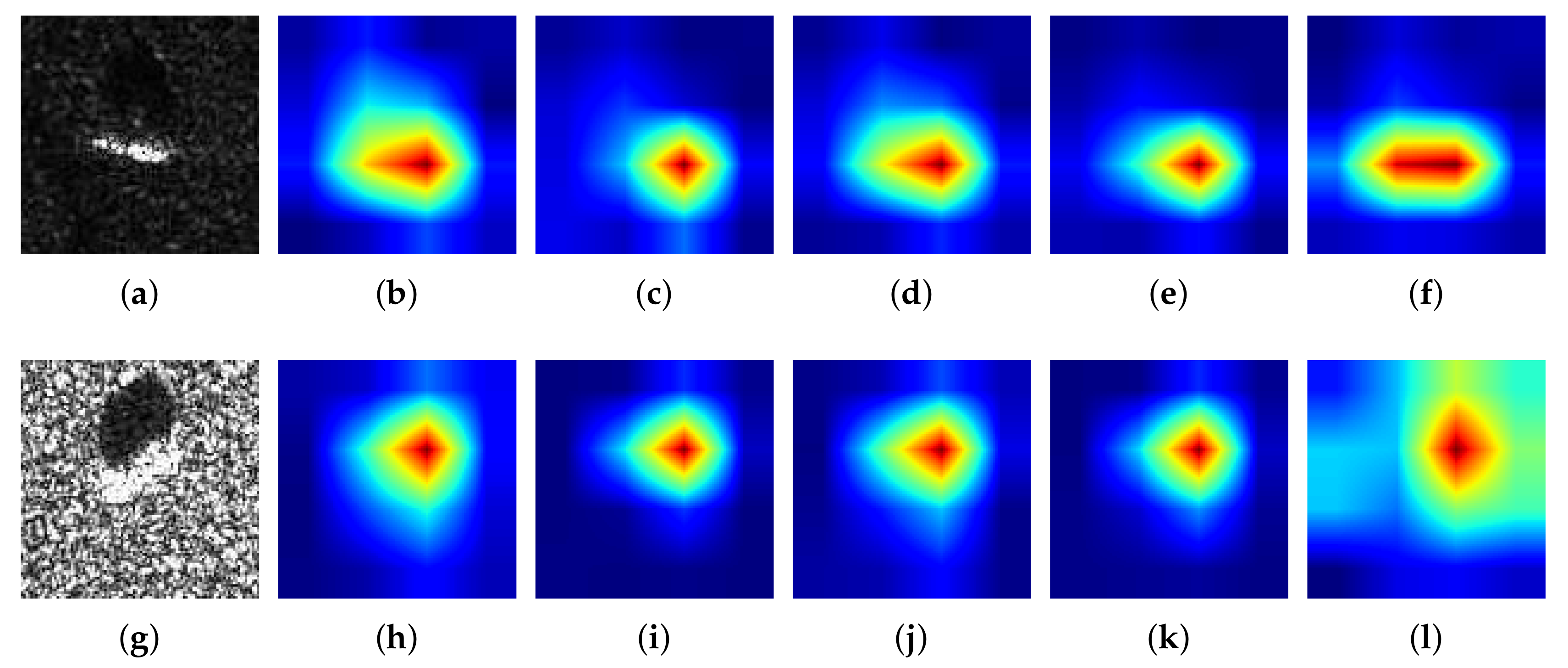
The validity of the aforementioned CAM methods has been demonstrated on various optical image datasets. However, SAR images are quite different from ordinary images: (1) the extra-class difference of SAR images is relatively smaller than that of optical images, e.g., the difference between an armored vehicle and a tank in the MSTAR dataset is evidently smaller than the difference between a dog and a ship in the CIFRA-1O dataset; (2) in comparison to optical images, SAR images have low resolution, low signal-to-noise ratio (SNR), and usually contain a number of interference spots. In this case, the heatmap generated by the above CAM methods designed for optical images usually cannot precisely locate the target in SAR images, which exhibits an irregular region overcovering the target. We randomly selected two SAR images from the MSTAR dataset and calculated their heatmaps corresponding to different CAM methods. The results are shown in Figure 1. It is evident that Grad-CAM++ and Ablation-CAM only locate parts of the target, while Grad-CAM, XGrad-CAM, and Score-CAM all overcover the target. In this case, class discrimination of the heatmaps will be reduced dramatically, meaning it is difficult to understand what the CNN learns to make it classify these targets corresponding to different classes.

3. Our Methodology

3.1. Inspiration and Motivation

As discussed in Section 2, neither gradient-based nor gradient-free CAM methods can provide a heatmap that covers the targets in SAR images precisely. As for gradient-based methods, it is still worth discussing whether using gradients as weights is reasonable. For gradient-free methods, they may be more suitable for high-resolution optical images because there usually exists abundant information like edge and texture, thus more sophisticated details can be abstracted in feature maps, whereas SAR images usually have much lower resolution than optical images. Therefore, it is very important to make full use of the information in the input image itself.

Except for Score-CAM, the rest of the methods all aim at designing weights ${\alpha }^{ck}$ by various artful manipulations but ignore the input image, which contains everything the CNN needs. Score-CAM defines the weights by calculating the similarity between feature maps and the input image. It is a good idea but it does not appear to be perfect for SAR images, as shown in Figure 1. Inspired by Score-CAM, we propose a novel CAM method named Self-Matching CAM, which is especially suitable for SAR images. It should be noted that Self-Matching CAM is not a modified version of Score-CAM even though the latter indeed inspired Self-Matching CAM. Specifically, it is not a new design of weight manipulation anymore, but is a post-processing framework that is implemented after available CAM methods and produces a high class-discriminative heatmap where the target is located precisely. The detailed procedures of Self-Matching CAM and the specific difference between it and Score-CAM will be elucidated in the following.

3.2. Self-Matching CAM

In Score-CAM, the feature maps need to be upsampled to the same shape with the input image according to Equation (14), and the CIC is calculated to measure the correlation of the feature map and the input image. No matter what kind of upsampling method is used, some irrelevant information will be introduced; inevitably, meanwhile, such an upsampling operation is required for every feature map. In this case, the irrelevant information will be accumulated many times, especially for a deep CNN with a large number of channels in a convolutional layer. To alleviate this problem, we downsample the input image to the same shape with feature maps instead of upsampling the feature maps. We assume I denotes the input SAR image, and this operation can be written as:

$$\begin{array}{c}\hfill \tilde{I}=s(Down(I))\end{array}$$

(16)

where $\tilde{I}$ denotes the downsampled input image in the same shape of the feature maps, and $Down$ denotes the downsampling operation. Compared with upsampling, downsampling can bring two advantages. (1) Downsampling will not introduce any irrelevant information. This operation only discards some details of the input image. (2) Downsampling needs to implement only once per image. After that, we calculate the Hadamard product of the input image and each feature map as a new group of modified feature maps. Then, the Hadamard product of the downsampled input and k-th feature map $A^k$ are used as a new feature map ${\widehat{A}}^k$, formulated as:

$$\begin{array}{c}\hfill {\widehat{A}}^k=A^k\circ \tilde{I}\end{array}$$

(17)

By substituting Equation (17) into Equation (2), we can obtain a heatmap generated from Self-Matching CAM as below:

$$\begin{array}{c}\hfill H_{ij}^{Self-Matching\_CAM}=\underset{k}{\mathsf{\Sigma }}{\alpha }^{ck}Up({\widehat{A}}_{ij}^k)\end{array}$$

(18)

where $H_{ij}^{Self-Matching\_CAM}$ refers to the element of $H^{Self-Matching\_CAM}$ in coordinates (i,j) and ${\alpha }^{ck}$ is any one of the weights generated by the various CAM methods mentioned above.

However, for some CNNs with deep convolutional layers or a large shape of the pooling windows, the feature maps in the last convolutional layer are a very compact size. In this case, the downsampling operation may lose too much information including some that is relevant to the target, thus here we make a compromise: we downsample the input image I and upsample the feature map $A^k$ to an intermediate shape between I and $A^k$. We set $I_N$ in the shape of $N\times N$, $A_M^k$ in the shape of $M\times M$ ($N>M$), and ${\tilde{I}}_Q$ and ${\tilde{A}}_Q$ in the shape of $Q\times Q$ ($M<Q<N$), which can be written as:

$$\begin{array}{cc}\hfill {\tilde{I}}_Q& =s(Down{(I_N)}_Q)\hfill \end{array}$$

(19)

$$\begin{array}{cc}\hfill {\tilde{A}}_Q^k& =s(Up{(A_M^k)}_Q)\hfill \end{array}$$

(20)

where $Down{(·)}_Q$ and $Up{(·)}_Q$ denote downsampling the shape of the input to $Q\times Q$, and upsampling the feature map to $Q\times Q$, respectively. Hence, Equation (17) can be rewritten as follows by substituting Equations (19) and (20):

$$\begin{array}{c}\hfill {\widehat{A}}_Q^k={\tilde{A}}_Q^k\circ {\tilde{I}}_Q.\end{array}$$

(21)

In this case, the final heatmap can be formulated as:

$$\begin{array}{c}\hfill H_N^{Self-Matching\_CAM}=\underset{k}{\mathsf{\Sigma }}{\alpha }^{ck}Up{({\widehat{A}}_Q^k)}_N\end{array}$$

(22)

where $Up{(·)}_N$ denotes upsampling the shape to $N\times N$. The rationale and entire flowchart for Self-Matching CAM are presented in Figure 2 and Algorithm 1.

Algorithm 1 Self-Matching CAM

Input: SAR image $I_N$, Model $f(·)$, class c, resize_shape Q Output: $H^{Self-Matching\_CAM}$ initialization: # get feature maps of the last convolutional layer $A_M\leftarrow f(I)$ ${\alpha }^{ck}\leftarrow A_M$, $f(I)$ $C\leftarrow$ the number of channels in $A_M$ # Downsample $I_N$ to ${\tilde{I}}_Q$, $M<Q<N$ ${\tilde{I}}_Q=s(Down{(I_N)}_Q)$ for k in $[0,\dots ,C-1]$ do  # Upsample and normalize $A_M^k$  ${\tilde{A}}_Q^k=s(Up{(A_M^k)}_Q)$  # Hadamard product  ${\widehat{A}}_Q^k={\tilde{A}}_Q^k\circ {\tilde{I}}_Q$ end # Generate heatmap $H_N^{Self-Matching\_CAM}\leftarrow \underset{k}{\mathsf{\Sigma }}{\alpha }^{ck}Up{({\widehat{A}}_Q^k)}_N$

In addition, to avoid confusion, we compare the difference between Self-Matching CAM and Score-CAM in detail. (1) Self-Matching CAM is a post-processing method implemented on the heatmaps of available CAM methods, while Score-CAM is directly used to generate a heatmap. (2) Self-Matching CAM aims at producing a group of new feature maps matching the input image, while Score-CAM aims at manipulating the weights of feature maps. (3) Self-Matching CAM does not involve the final classification score $S_c$, while Score_CAM needs to calculate $S_c$ for each feature map.

4. Experimental Results

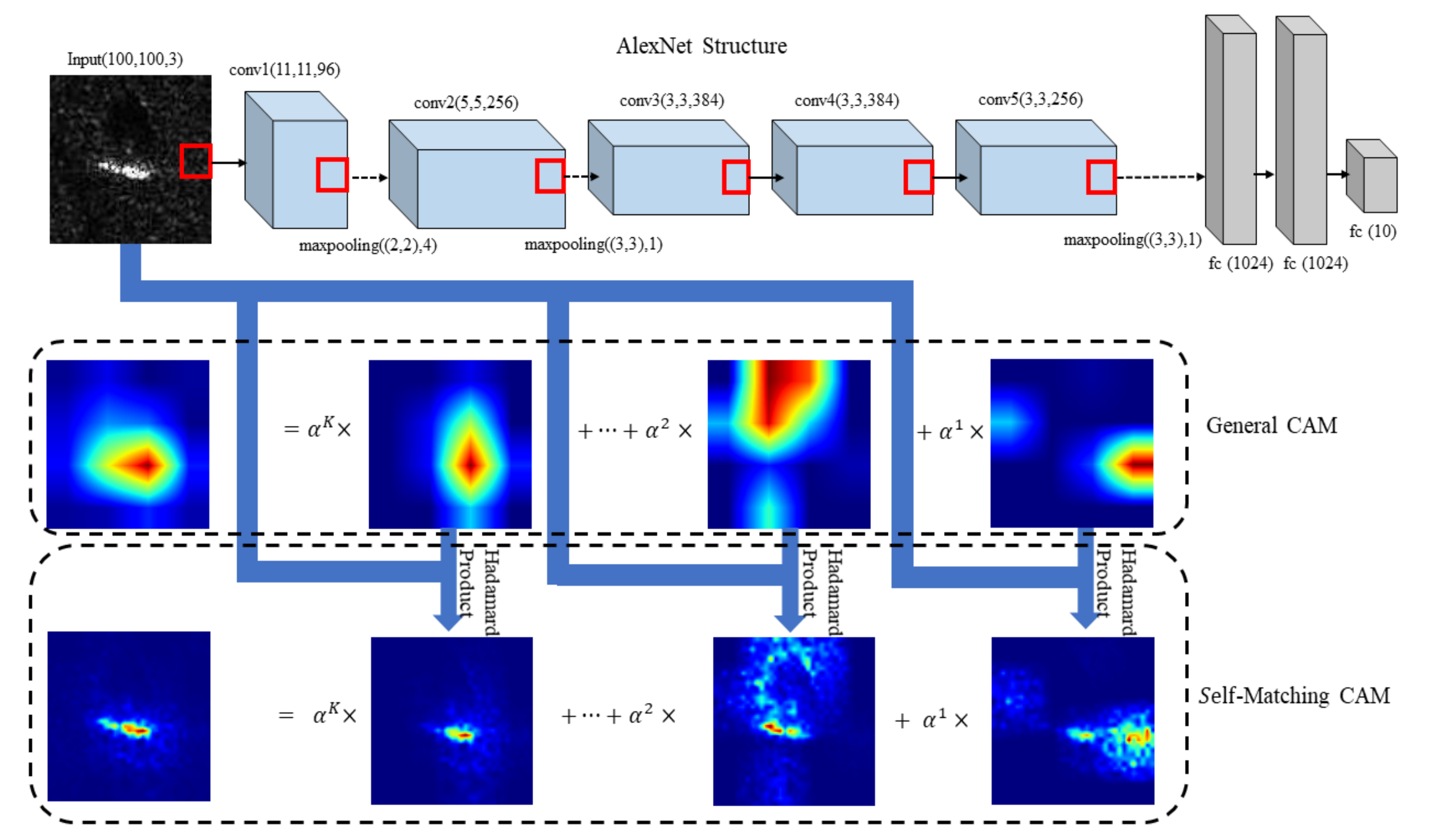
In this section, we will compare the effect of Self-Matching CAM with Grad-CAM, Grad-CAM++, XGrad-CAM, Ablation-CAM, and Score-CAM. We used AlexNet [30] as the CNN model, as shown in Figure 2 (stochastic gradient descent (SGD) was adopted as the optimizer, learning rate = $5\times {10}^{-4}$, momentum = $0.9$). MSTAR was adopted as a dataset that contains 2536 SAR images of 10 classes of vehicles for training and 2636 for validation. It is worth noting that the original SAR images are gray-scale; however, to avoid modification of the parameters of AlexNet, all the SAR images are transformed into pseudo-RGB images (reduplicate the monochromatic image in three channels). In this case, the parameters of AlexNet in Figure 2 are probably not the optimal set, e.g., the input size of an MSTAR image is $100\times 100$, while AlexNet is trained with images with a size of $224\times 224$. Note that the gist of this paper is to probe into this CNN to understand what information hidden in the input works on correct classification, but not the relationship between CAM effects and complex parameter tuning. In spite of this, AlexNet still obtains a high classification accuracy of $98.52\%$ after 270 epochs, which demonstrates that this set of parameters is effective. Without a special statement, the feature maps used in Self-Matching CAM are generated from XGrad-CAM due to its good performance compared to other methods in Figure 1. In addition, we conducted a perturbation analysis to further demonstrate that Self-Matching CAM can capture the most informative part of the target. Finally, we further studied how the highlighted region impacts CNN’s classification.

4.1. Qualitative Analysis

Figure 3 shows 10 SAR images of different targets and their corresponding heatmaps generated by Ablation-CAM, Score-CAM, Grad-CAM, Grad-CAM++, XGrad-CAM, and Self-Matching CAM. Qualitatively, it is intuitively evident that Self-Matching CAM outperforms other CAM methods dramatically. Only Self-Matching CAM can delineate the sophisticated edge of the target, while the other CAM methods can only provide a rough region. Score-CAM, Grad-CAM, and XGrad-CAM usually highlight a region that excessively covers the target, while Ablation-CAM and Grad-CAM++ highlight a narrow region that covers the target incompletely.

It is necessary to point out that the negative performance of other CAM methods does not mean the ineffectiveness of them. This is mainly because other CAM methods are designed for high-resolution optical images, particularly of multiple objects with abundant detailed information. Nonetheless, SAR images are quite different. (1) The resolution of SAR images is usually lower than that of optical images. (2) In MSTAR data, the target occupies only a small proportion of the image, whereas the objects usually occupy over half of optical images, like CIFRA 10 and ImageNet. In this case, the heatmaps generated by other CAM methods are difficult to locate on the target precisely though they are probably enough for optical images. In contrast, Self-Matching CAM is particularly designed on the basis of SAR image characteristics. The Hadamard product of the feature maps and input SAR image in Equation (21) is for retaining as much information relevant to the target itself as possible rather than some noise, like interference spots.

4.2. Quantitatively Analysis

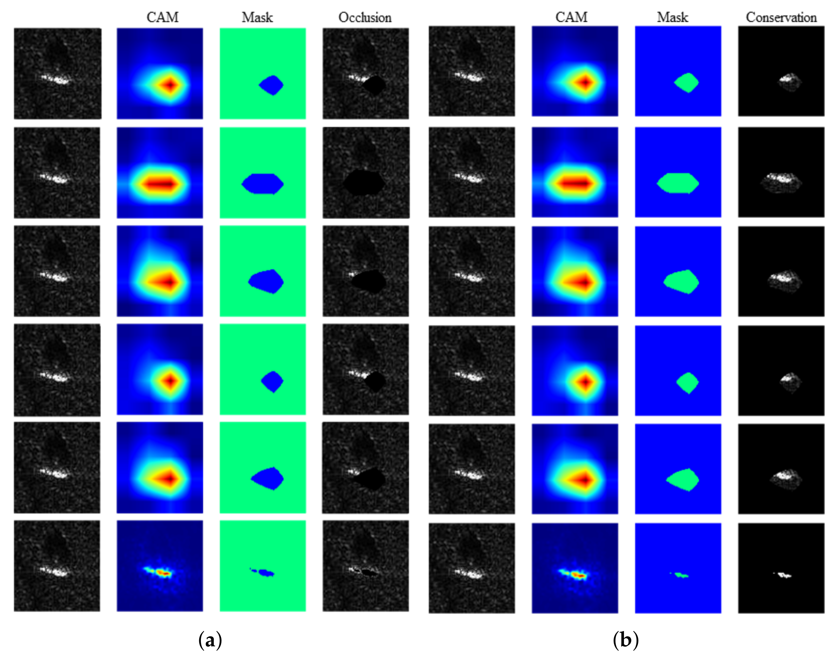
To analyze the localization capability of these CAM methods quantitatively, we implemented perturbation [19,26]. The underlying assumption is to occlude relevant/irrelevant regions in an input image to check the change of recognition accuracy. Specifically, perturbation can be categorized into an “occlusion test” and a “conservation test”. The occlusion test is used to measure how much of a region relevant to the target is included in the heatmap. In the occlusion test, we need to occlude the input image I by masking the region highlighted by the CAM method:

$$\begin{array}{cc}\hfill \check{I}=& I\circ (1-M^{Occlusion})\hfill \end{array}$$

(23)

where $\check{I}$ denotes perturbed image and $M^{CAM}$ denotes a binary-value mask defined as:

$$\begin{array}{c}\hfill \left\{\begin{array}{cc}{M}_{ij}^{Occlusion}=0,H_{ij}^{CAM}\ge 0.8,\hfill & \\ M_{ij}^{Occlusion}=1,H\mathrm{otherwise},\hfill & \end{array}\right.\end{array}$$

(24)

here $H_{ij}^{Occlusion}$ has been normalized to $[0,1]$. This means that in mask $M^{Occlusion}$, the elements corresponding to the top $20\%$ value of the heatmap are set to 0, while the rest are equal to the heatmap. Figure 4a shows the results of the occluded images.

Then, we can calculate the divergence of the class confidence (the output of the softmax layer) between the original image and the perturbed image:

$$\begin{array}{c}\hfill confidence\_drop(I,\check{I})=\frac{S_c(I)-S_c(\check{I})}{S_c(I)}\end{array}$$

(25)

In the occlusion test, a higher value of $confidence\_drop$ means that more parts of the target are included in the highlighted region in the heatmaps. We computed the average $confidence\_drop$ for all validation data (2636 SAR images) in MSTAR with the mentioned CAM heatmaps, which are shown in

Table 1. Class_drop for occlusion test.

Ablation	Score	Grad	Grad++	XGrad	Self-Matching
0.492	0.998	0.965	0.476	0.963	0.968

.

From Table 1, Ablation-CAM and Grad-CAM++ obtain very low $class\_drop$ compared with other methods. This indicates that these two methods cannot highlight parts of the target in the heatmap rather than the entire target region. In contrast, the $class\_drop$ values of the other methods are approximate to 1, which represents an entire coverage of the target. However, sometimes the highlighted region overcovers the target, like Score-CAM, Grad-CAM, and XGrad-CAM, as shown in Figure 3, which can also lead to a high value of $class\_score$ in the occlusion test in Table 1. To measure how much of the region that is irrelevant to the target is included in a heatmap, we also implemented a conservation test. The solitary difference between the conservation test and the occlusion test is the mask $M^{Conservation}$ formulation, defined as:

$$\begin{array}{c}\hfill M^{Conservation}=U-M^{Occlusion}\end{array}$$

(26)

where U is a matrix $\forall i,j$, $U_{ij}=1$. The results of the conservation test are shown in Figure 4b. Evidently, a conservation test is an opposite operation of an occlusion test, which conserves the highlighted region instead of occluding it. Thus, in a conservation test, a low value of $class\_drop$ implies a more precise localization capability for CAM methods. The average $class\_drop$ of 2636 SAR images in validation dataset is shown in

Table 2. Class_drop for conservation test.

Ablation	Score	Grad	Grad++	XGrad	Self-Matching
0.581	0.613	0.643	0.417	0.576	0.002

.

From Table 2, Score-CAM, Grad-CAM, and XGrad-CAM all obtain a high $class\_drop$ in the conservation test. This is probably because although they can cover the entire target, such an overcovered region may also introduce redundant information like numerous interference spots that exist in original images, which is negative for classification. In comparison, the $class\_drop$ for Self-Matching CAM is lower than that of the rest of the methods dramatically. A high $class\_drop$ in the occlusion test and a low $class\_drop$ in the conservation test demonstrate that Self-Matching CAM locates the target precisely in the heatmap. Such experimental results greatly match the intuition from Figure 3 and Figure 4.

4.3. Classification Analysis

In this section, we will discuss the difference between Self-Matching CAM and other CAM methods in view of classification mechanism. Here we can obtain a set of masked data by implementing a conservation test for all MSTAR data under different CAM heatmaps according to Equation (26). Here we view the heatmaps as filters that only pass the relevant pixels of the input SAR image, like [31]. Next, we train another AlexNet with the masked training data. Finally, the original data and the masked data are fed into these two CNNs for testing.

The classification accuracy is shown in Figure 5. Here, Network 1 denotes the network fed with original data and Network 2 denotes the network fed with masked data. Interestingly, Network 1 is unable to classify masked data in any case. It manifests that what Network 1 learned from original data is probably not truly relevant to the target but is some other “coincident” information. Note that it is not overfitting since Network 1 can achieve high accuracy for both training data and validation data. This phenomenon may be due to the fact that Network 1 learned some “coincident” discriminative information that is irrelevant to the target but exists in a different class. For example, to distinguish people’s gender, facial features are usually considered as reasonable rather than dress color; however, sometimes the latter works because of a coincidence that all women are in white and all men are in red in a specific dataset. In addition, it can be observed from Figure 5 that only the network trained with masked data generated by Self-Matching CAM can achieve more than $95\%$ accuracy for original data and masked data simultaneously. This further demonstrates that CNN really learned the most informative parts of the target in SAR images from masked data generated by Self-Matching CAM.

4.4. Generalization Analysis

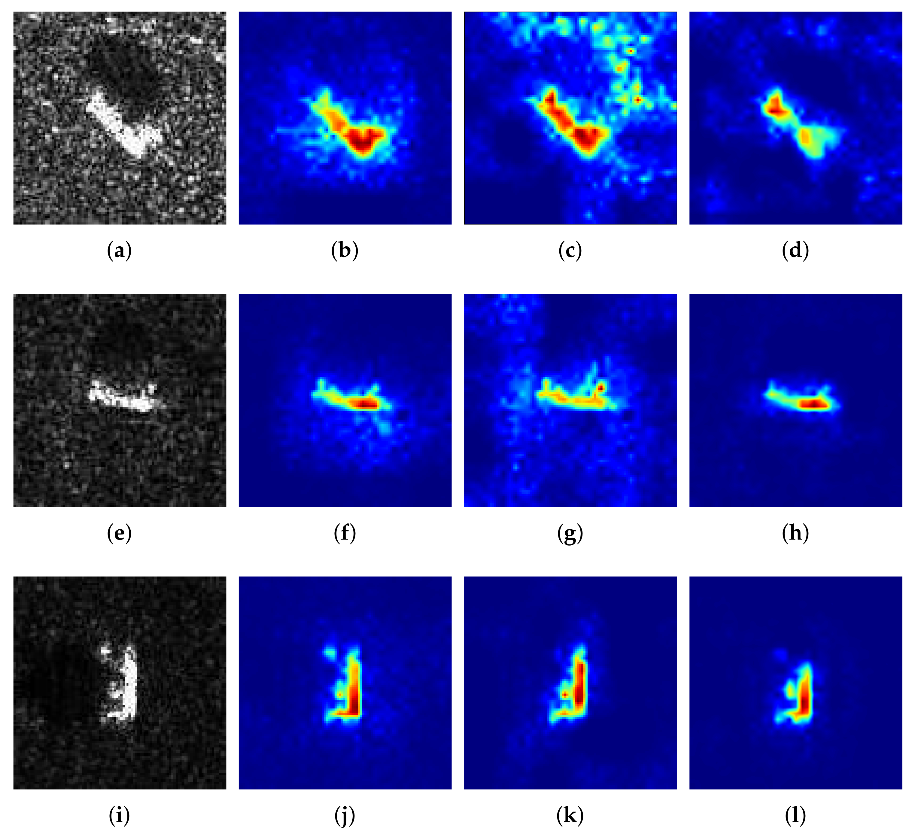
Although all the above experimental results are based on AlexNet, Self-Matching CAM actually achieves good generalization on multifarious CNN structures. In this section, we will perform Self-Matching CAM with another three famous CNN models besides AlexNet: VGG16, VGG19, and ResNet50. They can achieve a classification accuracy of $98.82\%$, $97.34\%$, and $72.84\%$, respectively. It is interesting that as the depth of the CNN increases, the accuracy of the CNN reduces gradually (VGG16 has 13 convolutional layers, VGG19 has 16 convolutional layers, and ResNet50 has 49 convolutional layers). Such results may mismatch people’s intuition since a deeper CNN usually outperforms a shallower one in traditional computer vision tasks. This is probably because the properties of SAR images are quite different from those of ordinary optical images, leading to a CNN’s different recognition mechanisms for them. However, this phenomenon implies the importance and necessity of explaining what CNN learns from the input SAR images.

The visualization results for ResNet50 are considered less convincing and reasonable in view of the low accuracy $72.84\%$, thus here only the Self-Matching CAM heatmaps based on AlexNet, VGG16, and VGG19 are shown in Figure 6. In general, Self-Matching CAM can highlight the target in the heatmap precisely for any one of three CNNs. In detail, some minor differences still exist: (1) VGG19 is the most robust to noise, AlexNet is in the middle, and VGG16 is the most sensitive to noise. This is probably because VGG19 has stronger abstraction ability in deeper convolutional layers, thus the feature maps in the last convolutional layer contain less information relevant to noise. (2) VGG19 does not highlight the target as completely as the other two CNNs. The reason is that the feature maps in VGG19 not only eliminate noise interference but also exclude parts of the information relevant to the target. The specific relationship between Self-Matching CAM and CNN structures is beyond the gist of this paper but it is worth future research.

5. Discussion

In our study, the effectiveness of Self-Matching CAM was verified from qualitative, quantitative, classification, and generalization analyses. Qualitative analysis provides an intuitive comparison of heatmaps generated by Self-Matching CAM and other CAM methods. It is clear that Self-Matching CAM can provide the most discriminative information that a CNN needs to make a classification. Quantitative analysis demonstrates such an intuition by a quantitative measurement: class_drop and two perturbation operations (occlusion and conservation). Furthermore, classification analysis indicates that Self-Matching CAM can enhance the robustness of a CNN and even improve accuracy slightly. Generalization analysis demonstrates that Self-Matching CAM can be applied to various CNN structures.

It should be also clarified that this paper aims at providing a visual explanation of CNN classification mechanisms but not designing an object extractor. Although some simple image processing algorithms, such as edge detection or target location, can probably profile the target in an SAR image, they are not correlated with a CNN’s inner products (feature maps) but are based on prior human cognition, such as the correlation between neighboring pixels, the sharp changes of gradient near an edge, etc. Hence, we have not compared Self-Matching CAM with them in this paper.

6. Conclusions

A Self-Matching CAM method that can provide a novel and accurate explanation of CNN for SAR image interpretation was proposed in this paper. Self-Matching CAM was inspired by Score-CAM originally but aims at generating a set of new feature maps matching the input image rather than complex manipulation on weights. Therefore, Self-Matching CAM is particularly suitable for SAR images whose resolution is low and the extra-class difference is not vivid as optical images. Besides, Self-Matching CAM is not an individual method but a framework that can be combined with various CAM methods, thus for other types of images, it is possible to obtain the optimal collocation by tuning the basis CAM method in Self-Matching CAM. In comparison to other state-of-the-art CAM methods, the proposed method can precisely highlight the regions most relevant to the target in the SAR image rather than a rough coverage. Numerous experimental results verify the validity of Self-Matching CAM through qualitative and qualitative analyses. Moreover, generalization analysis demonstrates that Self-Matching CAM can obtain acceptable results with different CNNs. Classification analysis indicates that a CNN can learn the information that is really relevant to the target instead of noise, interference, and other coincident information. This finding may help to understand the inner mechanism of CNN classification, which is our future research direction.