Mapping Riparian Habitats of Natura 2000 Network (91E0*, 3240) at Individual Tree Level Using UAV Multi-Temporal and Multi-Spectral Data

Abstract

Riparian habitats provide a series of ecological services vital for the balance of the environment, and are niches and resources for a wide variety of species. Monitoring riparian environments at the intra-habitat level is crucial for assessing and preserving their conservation status, although it is challenging due to their landscape complexity. Unmanned aerial vehicles (UAV) and multi-spectral optical sensors can be used for very high resolution (VHR) monitoring in terms of spectral, spatial, and temporal resolutions. In this contribution, the vegetation species of the riparian habitat (91E0*, 3240 of Natura 2000 network) of North-West Italy were mapped at individual tree (ITD) level using machine learning and a multi-temporal phenology-based approach. Three UAV flights were conducted at the phenological-relevant time of the year (epochs). The data were analyzed using a structure from motion (SfM) approach. The resulting orthomosaics were segmented and classified using a random forest (RF) algorithm. The training dataset was composed of field-collected data, and was oversampled to reduce the effects of unbalancing and size. Three-hundred features were computed considering spectral, textural, and geometric information. Finally, the RF model was cross-validated (leave-one-out). This model was applied to eight scenarios that differed in temporal resolution to assess the role of multi-temporality over the UAV’s VHR optical data. Results showed better performances in multi-epoch phenology-based classification than single-epochs ones, with 0.71 overall accuracy compared to 0.61. Some classes, such as Pinus sylvestris and Betula pendula, are remarkably influenced by the phenology-based multi-temporality: the F1-score increased by 0.3 points by considering three epochs instead of two.

1. Introduction

Riparian habitats are an interface between terrestrial and aquatic ecosystems along inland watercourses [1] and provide a series of ecological services important for the balance of the environments with which they come into contact (buffer effect against the loss of nutrients, purification of drainage water, anti-erosion action, consolidation of the banks, etc.) [2,3]. Riparian habitats develop on gravelly-sandy riverbeds with torrential regimes, with significant variations of the water table level during the year, and on alluvial soils are often flooded, features which often may hamper the evolution of the cenosis towards mature communities [4]. Such habitats’ strong dynamism is mirrored in a high vegetation structural complexity and, in turn, in a high taxa diversity. Indeed, according to the habitat heterogeneity hypothesis, such vegetation structural complexity provides several ecological niches and resources for a wide variety of species, thus supporting a high species richness [5]. In European countries, riparian habitats are subject to several kinds of human impact that are highly detrimental for biodiversity and, for this reason, they are included in the Directive 92/43/EEC (“Habitats Directive”). Currently, fifteen habitats are recognized in Italy, related both to standing water (lakes and ponds, Natura 2000 codes from 3110 to 3170*) and running water (river and torrents, Natura 2000 codes from 3220 to 3290) environments [6].

Moreover, “Alluvial forests with Alnus glutinosa and Fraxinus excelsior (Alno-Padion, Alnion incanae, Salicion albae)” (Natura 2000 code: 91E0*) are also considered to be priority habitats for biodiversity conservation [6]. The Habitat Directive requires the Member States to implement surveillance of the conservation status of habitats of Community Interest and, for Italy, a handbook with monitoring guidelines for all habitat types has been produced [4]. In this handbook, particular regard is paid to the data collection at site level. However, field-based inventories can be time-demanding, labor-intensive, and expensive due to the complex vegetation structure. Alternatively, remote sensing could be a valuable tool to overcome the difficulties of field surveys in exhaustively identifying shrub and tree species, and describing their spatial distribution in such environments. Indeed, remote sensing has become an efficient tool for identifying Natura 2000 Habitats, and gathering information on their conservation status and evaluating environmental policies’ implementation [7,8,9,10,11,12].

Today, a vast amount of remotely sensed data that offers useful information to map natural habitats is available [8,9,13]. The potential of remotely sensed data in identifying habitats, obtaining information on their distribution, and monitoring their conservation status, is a prominent research topic, for which applications can be organized into two levels [9]. The first level focuses on distinguishing broad physiognomic types, such as grass, shrub, and tree. Satellite information is the input data for most first level studies [7,8,9]. The second level deals with the distinctions within the physiognomic type (forests, grasslands, heathlands, and wetlands) [9]. In other words, the classification of the species within a specific physiognomic type is the focus of level two research, and has spread during the past 35 years. In particular, the tree species classification of forest habitats recorded an exponential increase in 2005–2015 [13] due to the diffusion of unmanned aerial vehicles (UAVs) and a new broad variety of sensors.

Certainly, the use of UAVs in forests and environmental monitoring is currently in an expansion phase [14,15,16,17,18,19,20,21,22], encouraged by the affordability of new systems and sensors [23]. Airborne multispectral [15,19,21,22,24], hyperspectral [16,17,20,25], and LiDAR (usually combined with optical sensors [14,18]) sensors represent the most recent and completed systems for species classification of natural habitats. The common point of such technologies is the production of very high resolution (VHR) data, which have introduced a new set of possibilities for classifying the Earth’s surface at finer levels of spatial detail, allowing the description of small objects. The optical information provided by hyperspectral and multi-spectral data is fundamental to determine the species spectral variability and discriminate vegetation species with artificial intelligence classifications.

Both hyperspectral and multi-spectral sensors have provided reliable results in forest habitats species mapping (

Table 1. Analyzed studies focusing on forest tree species recognition based on multi-spectral and hyperspectral data.

Study	Spectral Sensor	Number of Classes	Number of Bands	Overall Accuracy	Forest Type	Classification Approach	Classification Algorithm	Multi-Temporal
Modzelewska et al. (2020) [20]	Hyper	7 (2 conifers, 5 broadleaves)	451	70	Temperate	Pixel-based	SVM	No
Nevalainen et al. (2017) [25]	Hyper	4 (3 conifers, 1 broadleaf)	33	95	Boreal	Individual tree	RF and k-NN	No
Sothe et al. (2019) [17]	Hyper	12 (12 broadleaves)	25	72	Subtropical	Pixel-based	SVM	No
Takahashi Miyoshi et al. (2020) [16]	Hyper	8 (8 broadleaves)	25	50	Atlantic	Pixel-based	RF	Yes, on year bases (3 epochs)
Xu et al. (2020) [15]	Multi (+LiDAR)	8 (3 conifers, 5 broadleaves)	8	66	Subtropical	Individual tree	RF	No
Shi et al. (2020) [18]	Multi (+LiDAR)	5 (2 conifers, 3 broadleaves)	3	67 77 (with LiDAR)	Temperate	Individual tree	RF	Yes, on year bases (3 epochs)
Ferreira et al. (2020) [22]	Multi	4 (palms)	3	83 (averaged accuracy)	Amazon palms	Individual tree	CNN	No
Schiefer et al. (2020) [21]	Multi	14(5 conifers, 9 broadleaves, 2 other)	3	89	Temperate	Pixel-based	CNN	No
Francklin et al. (2017) [19]	Multi	5 (5 broadleaves)	6	78	Temperate	Object oriented	RF	No
Michez et al. (2016) [24]	Multi (+LiDAR)	5 (4 broadleaf, 1 other)	6	79	Temperate riparian	Object oriented	RF	Yes, non-phenological-based (25 epochs)

The number of classes, their nature, the sensor, the classification algorithm, the overall accuracy of the type of classified environment, the classification approach and the multi-temporality of the input dataset are described. When different methods were compared in the study, the best results are reported. SVM = support vector machine; RF = random forest; k-NN = k-neural networks; CNN = convolutional neural networks.

). The accuracy of the species classification is hugely influenced by the number of classes (i.e., the number of mapped species) and the complexity of the habitat, and less by the sensor’s nature. The classification approach also plays a crucial role in species discrimination (Table 1). Generally, pixel-based classifications perform better than the classification of species at the individual tree level. Much research has been carried out on the segmentation of single tree crowns (also referred to as individual tree detection, ITD) from VHR optical imagery derived from UAVs, which is considered a good data source for ITD. Despite being recognized as essential for habitat and biodiversity monitoring, resource inventories, wildlife habitat mapping, and management purposes [13,25], individual tree level information is underrepresented in the literature. This is partially due to the difficulties related to the segmentation of the individual crowns. Indeed, broadleaf tree species are generally more difficult to segment into coherent tree crowns than conifers, and tend to be classified with lower accuracies [23]. Variables such as topography, high stand density (i.e., resulting in the interpenetration of tree crowns), habitat heterogeneity, and small size crowns can further exacerbate individual trees’ segmentation. Most of these aspects characterize riparian habitats. Indeed, despite the spread of remote sensing in habitat monitoring and, more generally, in tree species classification, very few studies have been carried out on riparian areas. To the best of the authors’ knowledge, to date, only one study has been carried out to monitor riparian habitats at individual tree level using VHR UAV data (Table 1).

Multi-temporal approaches improve the final accuracies of vegetation species classification [13,16,24] and can mirror species’ phenology in the areas of the world in which the vegetation changes on a seasonal basis. The multi-temporal, or multi-date, approach’s main idea is to characterize objects by stacking the feature of the images acquired at different times. This method has been applied with a seasonal declination [26,27]. Namely, the multi-temporal datasets are created on a phenological, season, or biomass growing basis. However, the phenology is species-specific and requires botanical expertise [13]. Phenology-based multi-temporal study is widely explored for satellite-based remote sensing [13,24,28,29,30], but less applied in UAV-based analysis, although one of the most appreciated characteristics of UAVs is the high and customizable time resolution. To the best of the authors’ knowledge, most of the UAV studies for natural habitat species classification use multi-temporality regardless of the phenological information [16,18,24], and only obtain the advantages associated with the possibility of collecting UAV images in a period of particular interest (Table 1).

To assess if UAV-remote sensing can be an effective tool for mapping complex riparian habitats of the Natura 2000 network, we tested a multi-temporal phenological-based tree and shrub species classification at individual crown level, using multi-spectral information. The analyzed riparian habitats were 3240 (alpine rivers and their ligneous vegetation with Salix eleagnos) and 91E0* (riparian woods of Alnus incana of montane and sub-montane rivers of the Alps and the northern Apennines).

The aim of these tests was to use phenological- based multi-temporality to reduce the complexity of vegetation mapping in riparian environments.

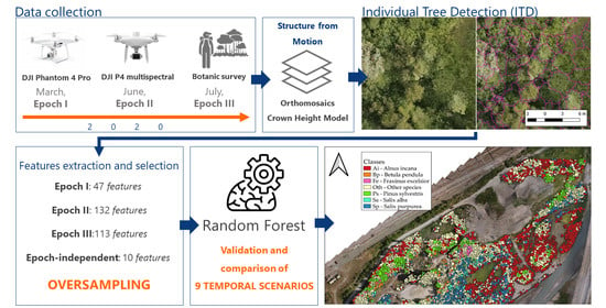
2. Materials and Methods

2.1. Study Area

The research was carried out in an alpine riparian area of the Dora Riparia river, in the Western Italian Alps (Salbertrand, Susa Valley—45.074000 N, 6.892200 E). The study site is an area of approximately 9 hectares located at an elevation of 1000 m a.s.l. (Figure 1). The climate is typically warm and temperate and, according to the meteorological station of the Regional Agency for the Protection of the Environment (ARPA Piemonte) located nearby at 1050 m a.s.l. (45.071204 N, 6.893979 E), the average annual temperature is about 8.2 °C and annual average precipitation is 701 mm (mean 1993–2017).

Dominating vegetation communities are mainly ascribable to two habitats of the Natura 2000 Network: 3240 (alpine rivers and their ligneous vegetation with Salix eleagnos) and 91E0* (riparian woods of Alnus incana of montane and sub-montane rivers of the Alps and the northern Apennines). Because the Habitat 3230 is an accessory series of 91E0*, these two habitats are often in catenal contact in mountain environments. Indeed, where alluvial events are most frequent, the typical occurring communities are related to Habitat 3240 (alliance Salicion incanae Aich. 1933). These formations have the ability to withstand both periods of over-enlargement and dry phenomena, and they were dominated by shrubby willows (mainly Salix eleagnos, Salix purpurea), by the Sea buckthorn (Hippophae rhamnoides), and by young individuals of Populus nigra. Conversely, areas less affected by alluvial events are characterized by hardwood-dominated vegetation communities (Habitat 91E0*), mainly ascribable to the alliances Salicion albae Soó 1930 and Alnion incanae Pawłowski in Pawłowski, Sokołowski and Wallisch 1928. In these communities, tree species (e.g., Salix alba, Fraxinus excelsior, Betula pendula, and Populus nigra) have a mature age and a considerable size. Several mature individuals of Pinus sylvestris are also present in the areas farther from the river, which characterize a transition community of the Habitat 91E0* towards a specific forest type recognized in Piedmont Region, named “River shores pinewood of Scots pine” [31,32].

2.2. UAV Data Collection

Very high resolution (VHR) optical data collected by multirotor UAV technology were employed to map the species of the studied riparian habitat. The choice of multirotor UAV and optical sensors for vegetation mapping was based on the characteristics of the study area, such as the topography, the extension, the presence of buildings, the climatic conditions, and the classification needs in terms of spatial and spectral resolution. The latter plays a crucial role in the classification of optical imagery. Indeed, the spectral information derived from the visible part of the electromagnetic spectrum alone is not enough to correctly discriminate the vegetation species. However, information regarding the non-visible part of the spectrum, such as the red edge and the near infra-red (NIR), strongly improves the classification and better describes the vegetation characteristics. Moreover, the red-edge and NIR information enhance the vegetation in the data and help to distinguish shadows within the tree crowns.

Three UAV campaigns were carried out in the study area at a vegetation-phenologically relevant time of the year. The first data collection campaign was conducted in March 2020 at the beginning of the green-up (epoch I); the second data acquisition occurred in June 2020 during the flowering of Salix spp. (epoch II); and the third in July 2020 (epoch III), during the crowns’ maximum development.

The surveyed area is larger than the classified area and also includes non-forested areas. Due to the large area surveyed and the need to carry multi-spectral optical sensors, which need a high payload capacity, we used two commercial multi-rotor solutions.

The first campaign (March) was conducted using the DJI Phantom 4 pro multirotor UAV device. An RGB optical camera with 12.4 megapixels and 8.8 mm focal length is embedded on the drone (

Table 2. UAV-embedded sensors‘ characteristics.

UAV	Sensors	Focal Length	Image Size	MP	Central Band and Bandwidth
DJI Phantom 4 multi-spectral	Multispectral	5.74 mm	1600 × 1300	2.08	R: 650 nm ± 16 nm G: 560 nm ± 16 nm B: 450 nm ± 16 nm REdge: 730 nm ± 16 nm N: 840 nm ± 26 nm
	RGB	5.74 mm	1600 × 1300	2.08	n.a.
DJI Phantom 4 pro	RGB	8.8 mm	4000 × 3000	12.4	n.a.

MP = megapixels; R = red; G = green; B = blue; REdge = red-edge; N = near-infrared; n.a. = not available.

). The UAV flew 98 m above the ground. The flights were manually operated, ensuring sufficient lateral and longitudinal overlaps within the frames (80% in both directions). The flights covered 1.2 km² and provided a 2.5 cm average ground sample distance (GSD).

The DJI Phantom 4 multi-spectral UAV was used in the June and July data collection campaigns. This model is a multirotor UAV with five multi-spectral sensors and an RGB sensor embedded. It has a multi-constellation and multi-frequency GNSS receiver in-built, which provides positioning accuracy of a few centimeters in RTK modality. The accurate positioning of the cameras’ frames allows the direct georeferencing of the photogrammetric block.

The multi-spectral sensors provide information in the red, green, blue, near-infrared (NIR) and red-edge electromagnetic spectra. They have a 5.74 mm focal length and 2.08 megapixels. The RGB sensor embedded on the DJI multi-spectral Phantom is a regular RGB camera with 5.74 mm focal length and 2.08 megapixels (Table 2).

The flights in June and July were manually operated at, respectively, 93 and 88 meters of altitude. As per the March flights, the overlap was manually ensured at around 80%. Two flights were conducted in June and July to cover the entire study area. The June flights resulted in 1332 frames with an average GSD of 4.7 cm, realized in about 3 h. In comparison, the July flights provided 1066 frames of 4.5 cm GSD.

Table 3. Characteristics of the three flights. GSD = ground sample distance.

	Epoch I	Epoch II	Epoch III
Number of flights	2	1	2
Date	17 March 2020	05 June 2020	27 July 2020
Average height (m)	98	93	88
Average GSD (m)	2.5	4.7	4.5
Area (km2)	1.2	0.59	0.78
Number of images	1100	1332	1066
Camera orientation	Nadiral, oblique	Nadiral, oblique	Nadiral, oblique

recaps the main characteristics of the data collection campaigns.

2.3. UAV Data Processing

The UAV-collected data were elaborated in orthomosaics using a standard structure from motion (SfM) workflow [33]. This process was undertaken using AMP (Agisoft Metashape Professional, Saint Petersburg, Russia) proprietary software for SfM [34]. In AMP, the alignment of images, the three-dimensional point cloud computation, the texture reconstruction, the mesh generation, and the orthomosaic generation were realized for each sensor acquisition. Moreover, the point cloud’s ground points were identified using an AMP inbuilt classification algorithm and the digital terrain model (DTM) generated by interpolating the ground points. From the three-dimensional point cloud, the digital surface model (DSM) was also computed. The data of each epoch were separately processed.

AMP can deal with multiband information; thus, the SfM elaborations resulted in one RGB orthomosaic, a DTM and a DSM for each epoch, and an additional multiband orthomosaic derived from the multi-spectral sensor of DJI Phantom 4 for epoch II and epoch III. The same acquisition images were separately analyzed on a sensor basis (Table 1).

Due to the embedded GNSS dual-frequency receiver, the three-dimensional models were directly georeferenced in the WGS84-UTM 32 coordinate system, applying the so-called “direct-photogrammetry” [35]. Nevertheless, to check the UAV-embedded GNSS measures’ final accuracy and improve the images’ alignment and the 3D model, 29 points were measured with a dual-frequency GNSS receiver. The points were well recognizable from the UAV pictures and measured using the NRTK GNSS technique. The measures reached 3 cm accuracy on the Up component and 1.5 cm on East and North components, with fixed-phase ambiguities for all points. Sixteen points were used as ground control points (GCPs) to georeference the 3D model, and thirteen points were employed as control points (CPs) to evaluate the georeferencing accuracy.

2.4. Identification and Mapping of Tree and Shrub Species

To train and validate the classification of crowns, a georeferenced database of tree and shrub species was first compiled. Using a GPS device with orthomosaics as background, botanists identified in the field the individual whose crowns were easily detectable from orthophotos. Then, botanists recorded the positions of these individuals by georeferencing the centroid of their crown directly on the GPS device. Each individual was identified at a species level, following the nomenclature of Pignatti (1982). In total, 268 tree and shrub samples were identified (

Table 4. Species mapped in the field and number of samples.

Species	Common Name	Code	Number of Samples
Alnus incana	Grey Alder	Ai	84
Salix purpurea	Red Willow	Sp	52
Salix alba	White Willow	Sa	40
Pinus sylvestris	Scots Pine	Ps	22
Betula pendula	Silver Birch	Bp	15
Fraxinus excelsior	European Ash	Fe	9
Elaeagnus rhamnoides	Sea Buckthorn	Er	8
Populus deltoides	Eastern Cottonwood	Pd	8
Salix eleagnos	Bitter Willow	Se	6
Populus canadensis	Canadian Poplar	Pc	5
Populus alba	White Poplar	Ppa	4
Larix decidua	European Larch	Ld	3
Populus nigra	Black Poplar	Pn	3
Buddleja davidii	Butterfly Bush	Bd	3
Salix triandra	Almond Willow	St	2
Prunus avium	Sweet Cherry	Pa	2
Populus tremula	European Aspen	Pt	1
Acer opalus	Italian Maple	Ao	1

, Figure 1).

2.5. Species Classification

The arboreal and shrub-like species were identified through a semi-automatic object-oriented (OBIA) supervised machine-learning classification. OBIA classification has been proved to be remarkably accurate for VHR optical datasets [36], and it permits the discrimination not only of homogeneous areas (such the pixel-based classifications) but also of single unit objects (such as buildings, tree crowns, and crop fields) [37,38,39]. In this application, each object describes an individual single crown. The main steps of this approach are [37]:

(i)

Segmentation;

(ii)

Feature extraction and data preparation;

(iii)

Training and test datasets creation;

(iv)

Classification;

(v)

Feature selection;

(vi)

Validation.

2.5.1. Segmentation

The segmentation was realized based on three-dimensional information of visible spectral information imagery, spectral indices, and textural analysis. The crown height model (CHM) was calculated as the difference between the DSM of epoch III and the DTM of epoch I, as Equation (1) shows:

CHM = DSM (III) − DTM (I)

(1)

The CHM represents the height of trees and shrubs of the dominant layer and constitutes the three-dimensional data for the segmentation. The DTM of epoch I was chosen because more ground points were available, whereas the DSM of epoch III was selected because it shows the maximum extension of crowns.

The Haralick measures based on the co-occurrence grey level matrix (CGLM) [40] were computed respectively on the green and NIR bands of epoch III. Precisely, the mean and the variance measures were calculated over a 5 × 5 pixel neighborhood. The choice of epoch III ensured segmentation on the maximum seasonal extension of the crowns. The normalized difference vegetation index (NDVI) of epoch II was computed and used to mask non-forested areas. The reason for the choice of epoch II for the NDVI index was because in June the trees and shrubs were in seasonal green-up, but the herbaceous vegetation was still in early stages of development and had low photosynthetic activity.

The segmentation of single trees and shrubs was performed in the eCognition Developer (Trimble) environment [41]. First, the forested area was selected by thresholding the NDVI at 0.12 and the CHM at 0.5 m. The non-forested areas smaller than 100 pixels were sieved. Then, the single crowns were defined by the multi-resolution segmentation algorithms. The input data were the CHM, the green band from epoch I, the blue and green bands from epoch II, and the textural bands of epoch III.

OBIA multi-resolution algorithms merge contiguous pixels into objects (i.e., groups of pixels) based on three user-defined parameters: scale, shape, and compactness. The scale represents the degree of spectral heterogeneity allowed in each object. Generally, the higher the scale value, which is unitless, and more extensive the object, the greater the heterogeneity [36,39]. The compactness parameter optimizes the resulting objects regarding their similarity to a circumference, whereas the shape describes the predominance of the geometry information over the spectral information.

The scale parameter was set to 25 and the shape and compactness 0.5 and 0.7, respectively. The segmentation step plays a crucial role in ITD-based classifications, and needs to be assessed as per the classification results. A qualitative and quantitative assessment based on the works of Persello et al. and Yurtseven et al. [42,43] was applied, similar to the analysis proposed in Belcore et al. [44].

One-hundred reference crowns were manually described using epoch III as a reference. The producer’s and user’s accuracy and the F1-score were calculated considering matched and omitted crowns [44]. The under-segmentation index (US), the over-segmentation index (OS), the completeness index (D), and the Jaccard index (J) were computed, in addition to the root mean square error (RMSE) over the area and the perimeter.

2.5.2. Feature Extraction

The feature extraction process generates new classification variables by combining information from the original features to provide more meaningful information than that contained in the original variables [45,46]. The diversification of the input features is crucial for accurate classification and some features, such as textural elements and spectral indices, have been proven to be good discriminants in image classification [47,48,49,50]. Once the crowns were delineated and assessed, the datasets were prepared for the classification and spectral, textural, and statistical features extracted for each crown. The features feeding the classification were textural-based, index-based, histogram-based, spectral-based, and elevation-based.

Table 5. Features of the classification. X indicates if the feature was calculated for I (epoch I), II (epoch II), and III (epoch III).

	Features	Formula/Notes	I	II	III
Spectral indices	Enhanced Vegetation Index (EVI)	$2.5\times \frac{\mathrm{B}9-\mathrm{B}5}{\mathrm{B}9+6\times \mathrm{B}5-7.5\times \mathrm{B}1}+1$		X	X
	Hue (RGB)	${\tan }^{-1}\frac{2\times \mathrm{Red}-\mathrm{Green}-\mathrm{Blue}}{30.5}\times \left(\mathrm{Green}-\mathrm{Blue}\right)$	X
	Hue multi-spectral	${\tan }^{-1}\frac{2\times \mathrm{RedEd}-\mathrm{NIR}-\mathrm{Red}}{30.5}\times \left(\mathrm{NIR}-\mathrm{Red}\right)$		X	X
	Intensity (RGB)	$\left(\frac{1}{30.5}\right)\times \left(\mathrm{Red}+\mathrm{Green}+\mathrm{Blue}\right)$	X
	Intensity multi-spectral	$\left(\frac{1}{30.5}\right)\times \left(\mathrm{RedEd}+\mathrm{NIR}+\mathrm{Red}\right)$		X	X
	Saturation (RGB)	$\frac{\max \left(\mathrm{Red}, \mathrm{Green}, \mathrm{Blue}\right)-\min \left(\mathrm{Red}, \mathrm{Green}, \mathrm{Blue}\right)}{\max \left(\mathrm{Red}, \mathrm{Green}, \mathrm{Blue}\right)}$	X
	Saturation multi-spectral	$\frac{\max \left(\mathrm{RedEd}, \mathrm{NIR}, \mathrm{Red}\right)-\min \left(\mathrm{RedEd}, \mathrm{NIR}, \mathrm{Red}\right)}{\max \left(\mathrm{RedEd}, \mathrm{NIR}, \mathrm{Red}\right)}$		X
	Normalized Difference Vegetation Index (NDVI)	$\frac{\left(\mathrm{NIR}-\mathrm{Red}\right)}{\left(\mathrm{NIR}+\mathrm{Red}\right)}$		X	X
	Normalized Difference Water Index NIR, (NDWI)	$\frac{\left(\mathrm{Green}-\mathrm{NIR}\right)}{\left(\mathrm{Green}+\mathrm{NIR}\right)}$		X	X
	Normalized Difference Water Index RedEdge (NDWI)	$\frac{\left(\mathrm{Green}-\mathrm{RedEd}\right)}{\left(\mathrm{Green}+\mathrm{RedEd}\right)}$		X	X
	Brightness	/	X
Histogram-based	Mode	Mode of the DN values of the polygon’s pixels.	X	X	X
	Mean	Mean of the DN values of the polygon’s pixels.	X	X	X
	Skew	Skewness of the DN values of the polygon’s pixels.	X	X	X
	Stdv	Standard deviation of the DN values of the polygon’s pixels.	X	X	X
GLCM textural measures	Contr	Contrast; measures the local contrast of an image.	X	X	X
	Entr	Entropy.	X	X	X
	Asm	Angular Second Moment; measures the number of repeated pairs.	X	X	X
	Corr	Correlation; measures the correlation between pairs of pixels.	X	X	X
	Idm	Inverse Difference Moment; measures the homogeneity.	X	X	X
	Savg	Sum Average.	X	X	X
	Svar	Sum Variance.	X	X	X
	Mean	Mean.	X	X	X
	Diss	Dissimilarity.	X	X	X
2nd order segmentation textural measures	Density of sub-objects	Standard deviation and mean of the density of the sub-object of a segment.	EPOCH-INDEPENDENT VARIABLE
	Direction of sub-objects	Standard deviation and mean of the main direction of the sub-object of a segment.
	Area of sub-objects	Standard deviation and mean of the areas of the sub-object of a segment.
	Asymmetry of sub-objects	Standard deviation and mean of the assymetry of the sub-object of a segment.
	Mean of sub-objects	Mean of of the sub-objects internal standard deviations calculated on the DN values.
	Avrg. mean diff to neighbors of sub-objects	Average difference of DN of each sub-object to the neighbouring ones.
	Max. diff.	Maximum difference of DN of the sub-objects.
DEM	CHM	Crown height elevation model	EPOCH-INDEPENDENT

summarizes the input metrics.

The enhanced vegetation index (EVI), the normalized difference vegetation index (NDVI), the normalized difference water index (NDWI), the saturation, the intensity, and the hue value was computed for each epoch. In particularly, the red, red-edge, and NIR information was input for the computation of saturation, intensity, and hue of epochs II and III.

The statistical features included the mean, mode, skewness, and standard deviation values of each available band.

Two types of texture were considered in the analysis: the Haralick-derived measures over the co-occurrence grey level matrix calculated on each crown’s pixels, and the texture based on sub-level segmentation. The angular 2nd moment, the contrast, the correlation, the dissimilarity, the entropy, and the homogeneity were the computed measures for each band. A sub-level segmentation was performed by applying multi-resolution segmentation (scale 10, shape 0.1, compactness 0.3) over the epoch II green band. The mean and the standard deviation of the density, the direction, the area, and the asymmetry of the sub-object were computed.

Histogram-based and GLCM textural features were calculated for all of the available bands of each epoch. The mean and the standard deviation of the spectral and the elevation-based features were computed for each segment. The sub-level segmentation texture and the elevation were epoch-independent since they were computed on multi-epoch data fusion. Three hundred and two features constituted the final classification dataset (Table 5).

2.5.3. Data Preparation and Classification Algorithm

The features were exported from eCognition converted to comma separated value (CSV) format, and then examined in a Python environment using Pandas, NumPy, and Sklearn libraries [51,52,53]. The species information collected in the field was attributed to the relative object. First, the dataset was cleaned of the null values and the features scaled on a minimum–maximum basis. Samples outside the case study boundaries were excluded. The S. eleagnos and the Salix triandra classes, which have respectively 6 and 2 samples and are very similar from a textural and spectral point of view, were assimilated to S. purpurea in the class Salix spp. Then, the species with fewer than nine samples were merged in the class “Other species”. The data preparation resulted in 260 samples. As

Table 6. Classes of the classification and number of available samples.

Class (Species)	Common Name	Class Label	Number of Available Samples
Alnus incana	Grey Alder	Ai	82
Salix purpurea	Red Willow	Sp	59
Other species	/	Oth	39
Salix alba	White Willow	Sa	38
Pinus sylvestris	Scots Pine	Ps	19
Betula pendula	Silver Birch	Bp	14
Fraxinus excelsior	European Ash	Fe	9

shows, the dataset was strongly unbalanced: the dominant class (A. incana) has 82 samples compared to nine of the smallest class (F. excelsior).

Imbalanced datasets generally lead to biases in the classification, and for this reason, are avoided [54]. For large datasets, the most commonly used approach for balancing is downsampling, which consists of reducing the sample to the size of the smallest class [54]. In this specific classification, the downsampling technique would lead to a tiny dataset (only nine samples per class). An alternative solution is oversampling, which, in contrast to downsampling, creates synthetic samples for the smaller classes to reach an analyst-defined size [55]. The borderline synthetic minority oversampling technique (SMOTE) was applied for oversampling. The borderline SMOTE algorithm works similarly to the SMOTE algorithm: it considers the n neighbor samples for each class, and interpolates them to create synthetic data [56], and a reduced number of nearest neighbors (m) for the smallest classes. The number of chosen neighbors (n) was 8, and two for the smaller classes (m), and the number of samples to reach the larger class (Alnus incana) was computed for each class. The borderline SMOTE algorithm was applied only on the training dataset. The final training dataset was composed of 574 samples.

Classification

The random forest algorithm [57] has been demonstrated to be particularly suitable for VHR optical data compared to other machine learning classifiers [58] and was used to classify the riparian species of trees and shrubs. A random forest classifier with two-thousand trees was applied, using the Gini criterion for node splitting [57,59].

Feature Selection

Feature selection reduces the dimensionality of the input features by decreasing the number of features in the classification. It aims to identify and remove redundant information so that the dataset can include maximum information using the minimum number of features [60]. The Gini importance is easily combined with decision trees and sorts the features based on the Gini impurity criterion [61].

Random forest importance analysis based on the Gini criterion was calculated for each feature to reduce and optimize the classification model [59]. Features that influence the classification less than the Gini threshold identified by Equation (2) were excluded from the classification.

$$\mathrm{T} = 0.75\times {{\displaystyle \sum }}_{i=1}^n\frac{x_i}{n}$$

(2)

where T is the threshold; n is the number of input features; x_i is the importance of the feature calculated based on the Gini impurity criterion.

2.5.4. Validation

The main accuracy measures based on the error matrix were calculated: the precision, recall, and F1-score for each class, and the overall accuracy were computed. The model was cross-validated. Due to the small size of the field dataset, the leave-one-out (LOO) cross-validation algorithm was applied [62,63]. Cross-validation consists of splitting the dataset of n samples into k folds of equal size and using each fold in turn to test the model trained over the remaining folds. The assessment of the results is given by the average (or modal) value of the analyzed assessment measures. LOO is a k-fold cross-validation method in which k is equal to n [62]. Each fold’s validation measures can result in a 0 (wrong classified test sample) or 1 (correctly classified test sample). The average of the single-fold validations yields the final accuracy values. For this classification, LOO cross-validation was applied, and the precision, recall, and F1-score for each class, and the overall accuracy were computed and then averaged.

2.5.5. Multi-Temporal Assessment

The multi-temporal scheme followed is identified as a multi-date approach, and consists of stacking the input images of a different time (information collected from epochs I, II and III) and classifying the entire dataset [64].

To assess the role of multi-temporality, the classification workflow was repeated for seven scenarios (A–G,

Table 7. The evaluated scenarios. Epoch-independent features (second-order texture and elevation) are included in feature counting.

Scenarios	Dataset Composition	Number of Features
A	Epoch I	56
B	Epoch II	142
C	Epoch III	122
D	Epoch I and II	189
E	Epoch II and III	255
F	Epoch I and III	169
G	Epoch I, II and III	302
H	Epoch I, II and III, no CHM	301
I	Epoch I, II and III no SMOTE	302

). Scenarios H and I were computed to assess the effect of SMOTE and CHM on the classification accuracy. For each scenario, the validation was carried out, and then the results compared.

3. Results and Discussion

3.1. UAV Data Processing

The photogrammetric processing results were georeferenced orthomosaics with 8 cm of spatial resolution and centimeter-level accuracy. The edges of the images were clipped to facilitate the next steps. Figure 2 shows the orthomosaics in RGB of epochs I, II, and III.

3.2. Species Classification

3.2.1. Segmentation

The segmentation resulted in 7092 segments corresponding to single crowns. Figure 3 provides some examples of the segmentation results.

The qualitative assessment of the crowns provided positive results (

Table 8. Results of the qualitative segmentation assessment. The metrics are computed over 100 manually delimited reference crowns.

Qualitative Metric	Value
Producer’s accuracy	0.81
Users’ accuracy	0.61
F1 score	0.70
Omission	0.19
Commission	0.39

). The F1-score was 0.70, and the omission error was 0.19. The method tended to over-segment the crowns, as shown by the commission error of 0.39 (Table 8).

The indicators measuring the quantitative goodness of the segmentation confirm the results of the qualitative assessment. The over-segmentation index ranges from 0.02 (very good result) to 0.45 (bad result) with 0.17 as the median value (

Table 9. Results of the quantitative assessment indices for the segmentation.

	Over-Segmentation Index *	Under-Segmentation Index *	Completeness Index *	Jaccard Index
Average	0.18	0.21	0.22	0.67
Min	0.02	0.01	0.07	0.05
Max	0.45	0.95	0.67	0.90
Median	0.17	0.18	0.20	0.69

* Smaller values indicate a better segmentation.

). Similarly, the under-segmentation index has a median value of 0.18. Both indices’ results are acceptable, although not optimal. The completeness index, which relates the over- and under-segmentation indices, is 0.2, indicating the over- and under-segmentation indices smaller values represent better segmentation conditions. The Jaccard index, equal to 0.69, indicates good overall segmentation. The root mean square error (RMSE) of the segmented perimeter is 2.78 m over an average crown perimeter of 9.86 m, representing 28% (

Table 10. Results of the quantitative assessment RMSE for the segmentation.

Metric	RMSE	Average Value of Crown Size	%	Unit of Measure
Area	0.87	6.99	12%	m2
Peimeter	2.78	9.86	28%	m

). In contrast, the RMSE of the area is 0.87 m² over an average crowns’ extension of 6.99 m² (12%).

As previously mentioned, the ITD segmentation of broadleaves is challenging and a source of less accurate classification. Individual tree detection (ITD) is a complex area of study and a research topic in itself.

Although the suitability of segmentation is rarely evaluated in the classification of individual tree crowns, the results obtained from this segmentation appear to be in line with the literature [43,44,65,66].

3.2.2. Classification Results

The classification was performed on the nine scenarios (Table 7) and then validated using the LOOCV method.

Table 11. Results of the LOOCV for the nine proposed scenarios. OA = overall accuracy. Refer to Table 4 for the species codes.

Scenario	OA	Metric	Ai	Sp	Oth	Sa	Ps	Bp	Fe
A		Precision	0.64	0.53	0.47	0.79	0.59	0.25	0.11
	0.58	Recall	0.73	0.53	0.37	0.77	0.68	0.14	0.11
		F1	0.68	0.53	0.41	0.78	0.63	0.18	0.11
B		Precision	0.61	0.59	0.43	0.78	0.64	0.00	0.25
	0.59	Recall	0.77	0.51	0.34	0.79	0.74	0.00	0.22
		F1	0.68	0.55	0.38	0.78	0.68	0.00	0.24
C		Precision	0.66	0.53	0.65	0.74	0.54	0.22	0.11
	0.61	Recall	0.79	0.39	0.32	0.85	0.63	0.14	0.22
		F1	0.73	0.46	0.53	0.81	0.60	0.17	0.11
D		Precision	0.64	0.54	0.54	0.71	0.79	0.17	0.17
	0.61	Recall	0.79	0.53	0.39	0.77	0.79	0.21	0.11
		F1	0.72	0.51	0.45	0.74	0.79	0.10	0.13
E		Precision	0.68	0.66	0.72	0.88	0.65	0.40	0.42
	0.69	Recall	0.84	0.59	0.47	0.97	0.68	0.14	0.56
		F1	0.75	0.63	0.57	0.93	0.67	0.21	0.48
F		Precision	0.64	0.55	0.58	0.79	0.67	0.33	0.29
	0.63	Recall	0.82	0.49	0.39	0.87	0.74	0.14	0.22
		F1	0.72	0.52	0.47	0.83	0.70	0.20	0.25
G		Precision	0.71	0.68	0.68	0.88	0.83	0.50	0.45
	0.71	Recall	0.88	0.61	0.50	0.95	0.79	0.21	0.56
		F1	0.78	0.64	0.58	0.91	0.81	0.30	0.50
H		Precision	0.70	0.61	0.70	0.86	0.82	0.50	0.56
	0.70	Recall	0.84	0.59	0.50	0.95	0.74	0.29	0.56
		F1	0.76	0.60	0.58	0.90	0.78	0.36	0.56
I		Precision	0.61	0.58	0.58	0.88	0.78	1.00	0.20
	0.65	Recall	0.90	0.49	0.37	0.92	0.74	0.00	0.11
		F1	0.73	0.53	0.45	0.90	0.76	0.00	0.14

reports recall, precision, and F1 for each class and the overall accuracy of the classified datasets.

The importance calculated on dataset G reduced the features to 131. Figure 4 shows the visual representation of the classified area.

As shown in Table 11, the multi-epoch phenological-based classification approach clearly outperforms the single-epoch approached. The overall accuracy scores of scenarios A, B and C, which do not exceed 0.61, strongly confirm this finding. The precision and the recall of the species of single-epoch scenarios are low for some classes, such as F. excelsior and “Other species”. B. pendula is not detected in Scenario B.

Unexpectedly, the performance of the classification does not improve consistently in scenarios D, E and F, in which data of two epochs were processed. Only scenario E (June and July data) provides a remarkable improvement in the overall accuracy (0.69). Such a trend is reasonable if we consider that scenarios D and F lack non-visible spectral information from epoch I.

Moreover, epoch I describes the study area at the beginning of the green-up. Nevertheless, although its contribution is minor, epoch I improves the accuracy of the final classification. By comparing scenarios E (epochs II and III) and G (epochs I, II, and III), the overall accuracy increases from 0.69 to 0.71. Specifically, there is a noticeable improvement in the precision, and consequentially the F1-score, of the classes B. pendula (Bp) and P. sylvestris (Ps). The decrease in the false positive rate may be ascribable to a correct description of the two species’ phenology. Pinus sylvestris is an evergreen species and, in contrast to other species of the habitat, its crown is fully developed and photosynthetic in epoch I. In addition, B. pendula’s catkins appear early in spring and have a characteristic yellow color, which is appreciable from the orthophoto (Figure 5).

In addition to evaluating the multi-date classification approach of VHR imagery for riparian habitat mapping, the roles of the CHM and the SMOTE algorithm were evaluated, respectively, in scenarios H and I. The CHM has a decisive influence on the classification, as also indicated by the importance analysis: the CHM mean value is placed in position 45 of 302. Indeed, the classes that take more advantage of the CHM are P. sylvestris (generally higher than other species) and S. purpurea (generally shorter than other species that characterize the habitat). Unexpected behavior is recorded for the B. pendula and F. excelsior classes, which the CHM negatively affects.

The comparison of scenarios I and G (respectively, without and with SMOTE) proves the effectiveness of the borderline SMOTE algorithm in this particular application. An improvement of the F1-score from scenario I to scenario G is detected for all classes, and the represented classes without training (B. pendula and F. excelsior) significantly benefit from the SMOTE (plus 0.30 on the F1 score from scenario I to G, Figure 6).

As Figure 6 shows, in general, the classification’s performance is proportional to the temporal information available. The classes of S. alba, A. incana, and P. sylvestris are better classified and represented by the model, followed by S. purpurea and the “Other Species” class. The B. pendula and F. excelsior classes are the least accurate. The S. alba (Sa) class outperform other classes in almost every analyzed scenario. This is ascribable to the unique color (and thus spectral response) of its leaves, which appear white-grey due to the fine pubescence covering the leaves’ surface.

As mentioned in the introduction, few studies have addressed the issues of individual tree mapping of biodiversity-relevant riparian habitats with multi-temporal approaches. The most similar work was conducted by Michez et al. [24] (Table 1). They applied a thick multi-temporal classification using a random forest in riparian areas. They obtained 0.80 accuracy over five classes. However, they did not work at the individual tree level, but with small objects resulting from a multi-resolution automatic segmentation (OBIA approach). It is worth mentioning that they analyzed the information of 25 UAV flights undertaken between September and October, in six days of work, compared to three days undertaken in the present work.

Shi et al. [18] tested the role of LiDAR in individual tree classification. They used five classes in a central European mixed forest, achieving 0.77 overall accuracy using LiDAR data, and 0.66 using a multi-temporal and multi-spectral approach (Table 1). This part of Shi et al.’s work differs from the research presented here, mainly due to the non-phenological based multi-temporal approach, which resulted in lower accuracy over fewer classes.

Xu et al. [15] classified eight species in tropical forests at the individual tree level. Their approach is similar to the current work because the segmentation is undertaken with a multi-resolution algorithm, although they applied a single-epoch classification. They obtained impressive results on the segmentation (0.82 F1-score), but only 0.66 classification overall accuracy (Table 1).

In this framework, the individual tree and shrub species mapping of habitats 91E0*and 3240 of the Natura 2000 network is consistent with the scientific relevant literature on the topic. It is worth considering the study area’s complexity and the difficulties related to the field data collection. Some classes are not remarkably accurate (B. pendula and F. excelsior), mainly due to the inadequate number of field samples and their low frequency in the area. The authors could have considered including F. excelsior and B. pendula in the “Other species” class (Oth), but mapping their presence was fundamental because they are species of physiognomic reference in 91E0* and 3240 Natura 2000 Habitats. Lidar technologies could improve the classification of B. pendula; indeed, the species has a characteristic crown shape due to slender and pendulous twigs. Similarly, enhancing the spectral detail by integrating hyperspectral cameras could have played a key role in spectrally separating B. pendula and F. excelsior and, generally, improving the classification accuracy.

The present methodology could have taken advantage of additional phenological-relevant observations, for example, multispectral data collected during the autumn season and extra ground truth points, although these activities are resource- and time-consuming. Unlike other forested habitats, the photointerpretation of riparian habitat species from VHR orthophotos is exceptionally complicated, including for expert botanists, meaning the collection of training and testing datasets in the field is unavoidable. As previously mentioned, UAV LiDAR could improve the ITD, and also the classification, by using 3D features [18]. Hyperspectral information could ease the class separability, avoiding the computation of many features. Nevertheless, these technologies are commonly more expensive than multispectral sensors [67,68]. Moreover, they require UAV systems with high payload capacity, and are difficult to integrate on the same UAV; thus, this approach would require more flights than are undertaken in multispectral surveys.

The development of a habitat-specific classification model facilitates its transferability and application to other areas because the main characterizing species (i.e., classes) of 3240 and 91E0* are modelled. The same methodology can be applied to larger areas, also using a different multispectral sensor. For larger areas, the use of fixed-wing drone systems is recommended, and the proposed classification model should be applied after the identification and localization of habitats 3240 and 91E0*.

4. Conclusions

This work aimed to assess the role of phenological-based multi-temporal tree and shrub species classification at the individual level in complex riparian Natural 2000 habitats (i.e., 3240 and 91E0*) using multi-spectral information. The results showed that the multi-temporality from the UAV positively responded to the classification requirements, allowing tree and shrub species to be mapped accurately and their spatial distribution to be characterized. These features are necessary to implement surveillance of the conservation status of Natura 2000 riparian habitats. The scenario with data from three epochs provided overall accuracy of 0.71, which is consistent with the existing literature on the topic.

The segmentation process strongly influenced the classification results and can be further improved. Indeed, the segmentation of VHR imagery is a challenging research topic, including in non-individual tree applications. Future studies should address this issue and attempt to integrate LiDAR data to identify individual crowns. Additionally, more field samples can be collected to test the same approach on a balanced and more significant training dataset.

The phenology-based multi-temporal approach is effective but requires good knowledge regarding the study habitat from ecological and botanical perspectives. Moreover, even with an in-depth knowledge of the habitat, analysis is required to find the balance between the available resources necessary for the UAV flights and the number of flights needed to correctly represent the phenology stages.

References

1. Naiman, R.J.; Décamps, H. The Ecology of Interfaces: Riparian Zones. Annu. Rev. Ecol. Syst. 1997, 28, 621–658. [Google Scholar] [CrossRef] [Green Version]
2. Hughes, F.M.R.; Rood, S.B. Allocation of River Flows for Restoration of Floodplain Forest Ecosystems: A Review of Approaches and Their Applicability in Europe. Environ. Manag. 2003, 32, 12–33. [Google Scholar] [CrossRef] [PubMed]
3. Naiman, R.J.; Décamps, H.; McClain, M.E. Riparia—Ecology, Conservation and Management of Streamside Communities. Aquat. Conserv. Mar. Freshw. Ecosyst. 2007, 17, 657. [Google Scholar] [CrossRef]
4. Angelini, P.; Ministero dell’Ambiente e della Tutela del Territorio e del Mare, Italy; ISPRA. Manuali per il Monitoraggio di Specie e Habitat di Interesse Comunitario (Direttiva 92/43/CEE) in Italia: Habitat; ISPRA: Roma, Italy, 2016; ISBN 978-88-448-0789-4. [Google Scholar]
5. Bazzaz, F.A. Plant Species Diversity in Old-Field Successional Ecosystems in Southern Illinois. Ecology 1975, 56, 485–488. [Google Scholar] [CrossRef]
6. Biondi, E.; Blasi, C.; Burrascano, S.; Casavecchia, S.; Copiz, R.; El Vico, E.; Galdenzi, D.; Gigante, D.; Lasen, C.; Spampinato, G.; et al. Manuale Italiano di Interpretazione Degli Habitat (Direttiva 92/43/CEE) 2009; Direzione per la Protezione della Natura: Rome, Italy, 2009. [Google Scholar]
7. Frick, A.; Haest, B.; Buck, O.; Vanden Borre, J.; Foerster, M.; Pernkopf, L.; Lang, S. Fostering Sustainability in European Nature Conservation NATURA 2000 Habitat Monitoring Based on Earth Observation Services. In Proceedings of the 1st World Sustainability Forum, Web Conference, 7 November 2011; p. 724. [Google Scholar]
8. Vanden Borre, J.; Paelinckx, D.; Mücher, C.A.; Kooistra, L.; Haest, B.; De Blust, G.; Schmidt, A.M. Integrating Remote Sensing in Natura 2000 Habitat Monitoring: Prospects on the Way Forward. J. Nat. Conserv. 2011, 19, 116–125. [Google Scholar] [CrossRef]
9. Corbane, C.; Lang, S.; Pipkins, K.; Alleaume, S.; Deshayes, M.; García Millán, V.E.; Strasser, T.; Vanden Borre, J.; Toon, S.; Michael, F. Remote Sensing for Mapping Natural Habitats and Their Conservation Status—New Opportunities and Challenges. Int. J. Appl. Earth Obs. Geoinf. 2015, 37, 7–16. [Google Scholar] [CrossRef]
10. Schmidt, J.; Fassnacht, F.E.; Neff, C.; Lausch, A.; Kleinschmit, B.; Förster, M.; Schmidtlein, S. Adapting a Natura 2000 Field Guideline for a Remote Sensing-Based Assessment of Heathland Conservation Status. Int. J. Appl. Earth Obs. Geoinf. 2017, 60, 61–71. [Google Scholar] [CrossRef]
11. Prošek, J.; Šímová, P. UAV for Mapping Shrubland Vegetation: Does Fusion of Spectral and Vertical Information Derived from a Single Sensor Increase the Classification Accuracy? Int. J. Appl. Earth Obs. Geoinf. 2019, 75, 151–162. [Google Scholar] [CrossRef]
12. Carvajal-Ramírez, F.; Serrano, J.M.P.R.; Agüera-Vega, F.; Martínez-Carricondo, P. A Comparative Analysis of Phytovolume Estimation Methods Based on UAV-Photogrammetry and Multispectral Imagery in a Mediterranean Forest. Remote Sens. 2019, 11, 2579. [Google Scholar] [CrossRef] [Green Version]
13. Fassnacht, F.E.; Latifi, H.; Stereńczak, K.; Modzelewska, A.; Lefsky, M.; Waser, L.T.; Straub, C.; Ghosh, A. Review of Studies on Tree Species Classification from Remotely Sensed Data. Remote Sens. Environ. 2016, 186, 64–87. [Google Scholar] [CrossRef]
14. Zlinszky, A.; Deák, B.; Kania, A.; Schroiff, A.; Pfeifer, N. Mapping Natura 2000 Habitat Conservation Status in a Pannonic Salt Steppe with Airborne Laser Scanning. Remote Sens. 2015, 7, 2991–3019. [Google Scholar] [CrossRef] [Green Version]
15. Xu, Z.; Shen, X.; Cao, L.; Coops, N.C.; Goodbody, T.R.H.; Zhong, T.; Zhao, W.; Sun, Q.; Ba, S.; Zhang, Z.; et al. Tree Species Classification Using UAS-Based Digital Aerial Photogrammetry Point Clouds and Multispectral Imageries in Subtropical Natural Forests. Int. J. Appl. Earth Obs. Geoinf. 2020, 92, 102173. [Google Scholar] [CrossRef]
16. Takahashi Miyoshi, G.; Imai, N.N.; Garcia Tommaselli, A.M.; Antunes de Moraes, M.V.; Honkavaara, E. Evaluation of Hyperspectral Multitemporal Information to Improve Tree Species Identification in the Highly Diverse Atlantic Forest. Remote Sens. 2020, 12, 244. [Google Scholar] [CrossRef] [Green Version]
17. Sothe, C.; Dalponte, M.; de Almeida, C.M.; Schimalski, M.B.; Lima, C.L.; Liesenberg, V.; Miyoshi, G.T.; Tommaselli, A.M.G. Tree Species Classification in a Highly Diverse Subtropical Forest Integrating UAV-Based Photogrammetric Point Cloud and Hyperspectral Data. Remote Sens. 2019, 11, 1338. [Google Scholar] [CrossRef] [Green Version]
18. Shi, Y.; Wang, T.; Skidmore, A.K.; Heurich, M. Improving LiDAR-Based Tree Species Mapping in Central European Mixed Forests Using Multi-Temporal Digital Aerial Colour-Infrared Photographs. Int. J. Appl. Earth Obs. Geoinf. 2020, 84, 101970. [Google Scholar] [CrossRef]
19. Franklin, S.E.; Ahmed, O.S. Deciduous Tree Species Classification Using Object-Based Analysis and Machine Learning with Unmanned Aerial Vehicle Multispectral Data. Int. J. Remote Sens. 2018, 39, 5236–5245. [Google Scholar] [CrossRef]
20. Modzelewska, A.; Fassnacht, F.E.; Stereńczak, K. Tree Species Identification within an Extensive Forest Area with Diverse Management Regimes Using Airborne Hyperspectral Data. Int. J. Appl. Earth Obs. Geoinf. 2020, 84, 101960. [Google Scholar] [CrossRef]
21. Schiefer, F.; Kattenborn, T.; Frick, A.; Frey, J.; Schall, P.; Koch, B.; Schmidtlein, S. Mapping Forest Tree Species in High Resolution UAV-Based RGB-Imagery by Means of Convolutional Neural Networks. ISPRS J. Photogramm. Remote Sens. 2020, 170, 205–215. [Google Scholar] [CrossRef]
22. Ferreira, M.P.; de Almeida, D.R.A.; Papa, D.d.A.; Minervino, J.B.S.; Veras, H.F.P.; Formighieri, A.; Santos, C.A.N.; Ferreira, M.A.D.; Figueiredo, E.O.; Ferreira, E.J.L. Individual Tree Detection and Species Classification of Amazonian Palms Using UAV Images and Deep Learning. For. Ecol. Manag. 2020, 475, 118397. [Google Scholar] [CrossRef]
23. De Luca, G.; Silva, J.M.N.; Cerasoli, S.; Araújo, J.; Campos, J.; Di Fazio, S.; Modica, G. Object-Based Land Cover Classification of Cork Oak Woodlands Using UAV Imagery and Orfeo ToolBox. Remote Sens. 2019, 11, 1238. [Google Scholar] [CrossRef] [Green Version]
24. Michez, A.; Piégay, H.; Lisein, J.; Claessens, H.; Lejeune, P. Classification of Riparian Forest Species and Health Condition Using Multi-Temporal and Hyperspatial Imagery from Unmanned Aerial System. Environ. Monit. Assess. 2016, 188, 146. [Google Scholar] [CrossRef] [Green Version]
25. Nevalainen, O.; Honkavaara, E.; Tuominen, S.; Viljanen, N.; Hakala, T.; Yu, X.; Hyyppä, J.; Saari, H.; Pölönen, I.; Imai, N.N.; et al. Individual Tree Detection and Classification with UAV-Based Photogrammetric Point Clouds and Hyperspectral Imaging. Remote Sens. 2017, 9, 185. [Google Scholar] [CrossRef] [Green Version]
26. Hepinstall-Cymerman, J.; Coe, S.; Alberti, M. Using Urban Landscape Trajectories to Develop a Multi-Temporal Land Cover Database to Support Ecological Modeling. Remote Sens. 2009, 1, 1353–1379. [Google Scholar] [CrossRef] [Green Version]
27. Long, J.A.; Lawrence, R.L.; Greenwood, M.C.; Marshall, L.; Miller, P.R. Object-Oriented Crop Classification Using Multitemporal ETM+ SLC-off Imagery and Random Forest. GIScience Remote Sens. 2013, 50, 418–436. [Google Scholar] [CrossRef]
28. Gärtner, P.; Förster, M.; Kleinschmit, B. The Benefit of Synthetically Generated RapidEye and Landsat 8 Data Fusion Time Series for Riparian Forest Disturbance Monitoring. Remote Sens. Environ. 2016, 177, 237–247. [Google Scholar] [CrossRef] [Green Version]
29. Zhu, X.; Liu, D. Accurate Mapping of Forest Types Using Dense Seasonal Landsat Time-Series. ISPRS J. Photogramm. Remote Sens. 2014, 96, 1–11. [Google Scholar] [CrossRef]
30. Key, T.; Warner, T.A.; McGraw, J.B.; Fajvan, M.A. A Comparison of Multispectral and Multitemporal Information in High Spatial Resolution Imagery for Classification of Individual Tree Species in a Temperate Hardwood Forest. Remote Sens. Environ. 2001, 75, 100–112. [Google Scholar] [CrossRef]
31. Mondino, G.P. Boschi Planiziali a Pinus Sylvestris e Alnus Incana delle Alluvioni del Torrente Bardonecchia; Regione Piemonte: Alessandria, Italy, 1963. [Google Scholar]
32. Camerano, P.; Gottero, F.; Terzuolo, P.G.; Varese, P. Tipi Forestali del Piemonte; IPLA S.p.A., Regione Piemonte, Blu Edizioni: Torino, Italy, 2008. [Google Scholar]
33. Turner, D.; Lucieer, A.; Watson, C. An Automated Technique for Generating Georectified Mosaics from Ultra-High Resolution Unmanned Aerial Vehicle (UAV) Imagery, Based on Structure from Motion (SfM) Point Clouds. Remote Sens. 2012, 4, 1392–1410. [Google Scholar] [CrossRef] [Green Version]
34. Agisoft Metashape. Available online: https://www.agisoft.com/ (accessed on 12 February 2021).
35. Chiabrando, F.; Lingua, A.; Piras, M. Direct Photogrammetry Using UAV: Tests And First Results. In Proceedings of the ISPRS—International Archives of the Photogrammetry, Remote Sensing and Spatial Information Sciences, Rostock, Germany, 16 August 2013; Volume XL-1-W2, pp. 81–86. [Google Scholar]
36. Hussain, M.; Chen, D.; Cheng, A.; Wei, H.; Stanley, D. Change Detection from Remotely Sensed Images: From Pixel-Based to Object-Based Approaches. ISPRS J. Photogramm. Remote Sens. 2013, 80, 91–106. [Google Scholar] [CrossRef]
37. Lu, D.; Weng, Q. A Survey of Image Classification Methods and Techniques for Improving Classification Performance. Int. J. Remote Sens. 2007, 28, 823–870. [Google Scholar] [CrossRef]
38. Meneguzzo, D.M.; Liknes, G.C.; Nelson, M.D. Mapping Trees Outside Forests Using High-Resolution Aerial Imagery: A Comparison of Pixel- and Object-Based Classification Approaches. Environ. Monit. Assess. 2013, 185, 6261–6275. [Google Scholar] [CrossRef] [PubMed]
39. Rastner, P.; Bolch, T.; Notarnicola, C.; Paul, F. A Comparison of Pixel- and Object-Based Glacier Classification With Optical Satellite Images. IEEE J. Sel. Top. Appl. Earth Obs. Remote Sens. 2014, 7, 853–862. [Google Scholar] [CrossRef]
40. Haralick, R.M.; Shanmugam, K.; Dinstein, I. Textural Features for Image Classification. IEEE Trans. Syst. Man Cybern. 1973, SMC-3, 610–621. [Google Scholar] [CrossRef] [Green Version]
41. ECognition|Trimble Geospatial. Available online: https://geospatial.trimble.com/products-and-solutions/ecognition (accessed on 11 February 2021).
42. Persello, C.; Bruzzone, L. A Novel Protocol for Accuracy Assessment in Classification of Very High Resolution Images. IEEE Trans. Geosci. Remote Sens. 2010, 48, 1232–1244. [Google Scholar] [CrossRef]
43. Yurtseven, H.; Akgul, M.; Coban, S.; Gulci, S. Determination and Accuracy Analysis of Individual Tree Crown Parameters Using UAV Based Imagery and OBIA Techniques. Measurement 2019, 145, 651–664. [Google Scholar] [CrossRef]
44. Belcore, E.; Wawrzaszek, A.; Wozniak, E.; Grasso, N.; Piras, M. Individual Tree Detection from UAV Imagery Using Hölder Exponent. Remote Sens. 2020, 12, 2407. [Google Scholar] [CrossRef]
45. Maxwell, A.E.; Warner, T.A.; Fang, F. Implementation of Machine-Learning Classification in Remote Sensing: An Applied Review. Int. J. Remote Sens. 2018, 39, 2784–2817. [Google Scholar] [CrossRef] [Green Version]
46. Thyagharajan, K.K.; Vignesh, T. Soft Computing Techniques for Land Use and Land Cover Monitoring with Multispectral Remote Sensing Images: A Review. Arch. Comput. Methods Eng. 2019, 26, 275–301. [Google Scholar] [CrossRef]
47. Jin, Y.; Liu, X.; Chen, Y.; Liang, X. Land-Cover Mapping Using Random Forest Classification and Incorporating NDVI Time-Series and Texture: A Case Study of Central Shandong. Int. J. Remote Sens. 2018, 39, 8703–8723. [Google Scholar] [CrossRef]
48. Lewiński, S.; Aleksandrowicz, S.; Banaszkiewicz, M. Testing Texture of VHR Panchromatic Data as a Feature of Land Cover Classification. Acta Geophys. 2015, 63, 547–567. [Google Scholar] [CrossRef] [Green Version]
49. Zhang, X.; Friedl, M.A.; Schaaf, C.B.; Strahler, A.H.; Hodges, J.C.F.; Gao, F.; Reed, B.C.; Huete, A. Monitoring Vegetation Phenology Using MODIS. Remote Sens. Environ. 2003, 84, 471–475. [Google Scholar] [CrossRef]
50. Drzewiecki, W.; Wawrzaszek, A.; Aleksandrowicz, S.; Krupiński, M.; Bernat, K. Comparison of Selected Textural Features as Global Content-Based Descriptors of VHR Satellite Image. In Proceedings of the 2013 IEEE International Geoscience and Remote Sensing Symposium—IGARSS, Melbourne, Australia, 21–26 July 2013; pp. 4364–4366. [Google Scholar]
51. McKinney, W. Data Structures for Statistical Computing in Python. In Proceedings of the 9th Python in Science Conference (SCIPY 2010), Austin, TX, USA, 28 June–3 July 2010; pp. 56–61. [Google Scholar] [CrossRef] [Green Version]
52. Harris, C.R.; Millman, K.J.; van der Walt, S.J.; Gommers, R.; Virtanen, P.; Cournapeau, D.; Wieser, E.; Taylor, J.; Berg, S.; Smith, N.J.; et al. Array Programming with NumPy. Nature 2020, 585, 357–362. [Google Scholar] [CrossRef]
53. Pedregosa, F.; Varoquaux, G.; Gramfort, A.; Michel, V.; Thirion, B.; Grisel, O.; Blondel, M.; Prettenhofer, P.; Weiss, R.; Dubourg, V.; et al. Scikit-Learn: Machine Learning in Python. J. Mach. Learn. Res. 2011, 12, 2825–2830. [Google Scholar]
54. Chawla, N.V. Data Mining for Imbalanced Datasets: An Overview. In Data Mining and Knowledge Discovery Handbook; Maimon, O., Rokach, L., Eds.; Springer: Boston, MA, USA, 2010; pp. 875–886. ISBN 978-0-387-09823-4. [Google Scholar]
55. Chawla, N.V.; Bowyer, K.W.; Hall, L.O.; Kegelmeyer, W.P. SMOTE: Synthetic Minority Over-Sampling Technique. J. Artif. Intell. Res. 2002, 16, 321–357. [Google Scholar] [CrossRef]
56. Han, H.; Wang, W.-Y.; Mao, B.-H. Borderline-SMOTE: A New Over-Sampling Method in Imbalanced Data Sets Learning. In International Conference on Intelligent Computing; Springer: Berlin/Heidelberg, Germany, 2005; Volume 3644, pp. 878–887. ISBN 978-3-540-28226-6. [Google Scholar]
57. Breiman, L. Random Forests. Mach. Learn. 2001, 45, 5–32. [Google Scholar] [CrossRef] [Green Version]
58. Belgiu, M.; Drăguţ, L. Random Forest in Remote Sensing: A Review of Applications and Future Directions. ISPRS J. Photogramm. Remote Sens. 2016, 114, 24–31. [Google Scholar] [CrossRef]
59. Hastie, T.; Tibshirani, R.; Friedman, J. Random Forests. In The Elements of Statistical Learning: Data Mining, Inference, and Prediction; Hastie, T., Tibshirani, R., Friedman, J., Eds.; Springer Series in Statistics; Springer: New York, NY, USA, 2009; pp. 587–604. ISBN 978-0-387-84858-7. [Google Scholar]
60. Campbell, J.B.; Wynne, R.H. Introduction to Remote Sensing, 5th ed.; Guilford Press: New York, NY, USA, 2011; ISBN 978-1-60918-176-5. [Google Scholar]
61. Ma, L.; Li, M.; Ma, X.; Cheng, L.; Du, P.; Liu, Y. A Review of Supervised Object-Based Land-Cover Image Classification. ISPRS J. Photogramm. Remote Sens. 2017, 130, 277–293. [Google Scholar] [CrossRef]
62. Kohavi, R. A Study of Cross-Validation and Bootstrap for Accuracy Estimation and Model Selection. IJCAI 1995, 14, 1137–1145. [Google Scholar]
63. Breiman, L.; Spector, P. Submodel Selection and Evaluation in Regression. The X-Random Case. Int. Stat. Rev. Rev. Int. Stat. 1992, 60, 291. [Google Scholar] [CrossRef]
64. Ghamisi, P.; Rasti, B.; Yokoya, N.; Wang, Q.; Hofle, B.; Bruzzone, L.; Bovolo, F.; Chi, M.; Anders, K.; Gloaguen, R.; et al. Multisource and Multitemporal Data Fusion in Remote Sensing: A Comprehensive Review of the State of the Art. IEEE Geosci. Remote Sens. Mag. 2019, 7, 6–39. [Google Scholar] [CrossRef] [Green Version]
65. Mohan, M.; Silva, C.A.; Klauberg, C.; Jat, P.; Catts, G.; Cardil, A.; Hudak, A.T.; Dia, M. Individual Tree Detection from Unmanned Aerial Vehicle (UAV) Derived Canopy Height Model in an Open Canopy Mixed Conifer Forest. Forests 2017, 8, 340. [Google Scholar] [CrossRef] [Green Version]
66. Vieira, G.d.S.; Rocha, B.M.; Soares, F.; Lima, J.C.; Pedrini, H.; Costa, R.; Ferreira, J. Extending the Aerial Image Analysis from the Detection of Tree Crowns. In Proceedings of the 2019 IEEE 31st International Conference on Tools with Artificial Intelligence (ICTAI), Portland, OR, USA, 4–6 November 2019; pp. 1681–1685. [Google Scholar]
67. Pearse, G.D.; Dash, J.P.; Persson, H.J.; Watt, M.S. Comparison of High-Density LiDAR and Satellite Photogrammetry for Forest Inventory. ISPRS J. Photogramm. Remote Sens. 2018, 142, 257–267. [Google Scholar] [CrossRef]
68. Vastaranta, M.; Kankare, V.; Holopainen, M.; Yu, X.; Hyyppä, J.; Hyyppä, H. Combination of Individual Tree Detection and Area-Based Approach in Imputation of Forest Variables Using Airborne Laser Data. ISPRS J. Photogramm. Remote Sens. 2012, 67, 73–79. [Google Scholar] [CrossRef]
Figure 1. Study area in Salbertrand, North-West Italy. The symbols show the species mapped in the field. The species codes are explained in Table 4.
Remotesensing 13 01756 g001
Figure 2. Detail of the orthomosaics of the RGB sensors resulting from the photogrammetric process. (a) Epoch I, March; (b) Epoch II, June; (c) Epoch III, July.
Remotesensing 13 01756 g002
Figure 3. Examples of the segmentation results. Different areas and different backgrounds: epoch II (bottom) and epoch III (above).
Remotesensing 13 01756 g003
Figure 4. Visual representation of the classification result.
Remotesensing 13 01756 g004
Figure 5. Detail of Pinus sylvestris (Ps) and Betula pendula (Bp) in epoch I (March). The other species (Bd and Pc) are still without leaves.
Remotesensing 13 01756 g005
Figure 6. F1-score variability in the analyzed scenarios.
Remotesensing 13 01756 g006