
Fractal Nature of Advanced Ni-Based Superalloys Solidified on Board the International Space Station


Abstract
:1. Introduction
1.1. Some Previous Results of Fractal Technique Application on Ceramics Samples
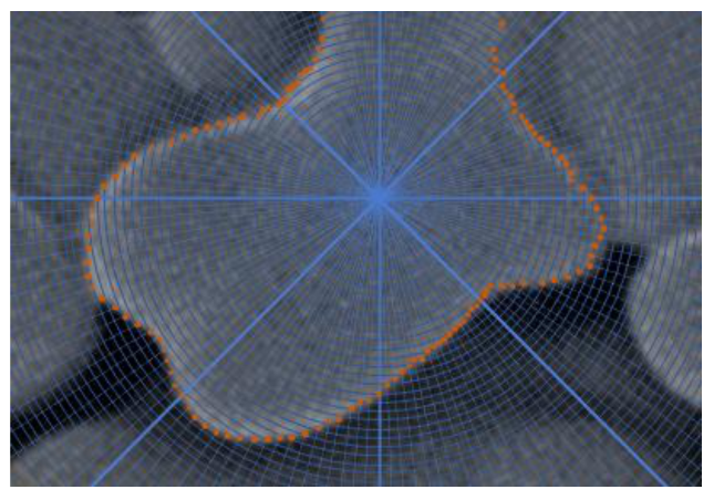
Short Description of the Applied Technique for the Grain Cluster Shape Reconstruction
2. Materials and Methods
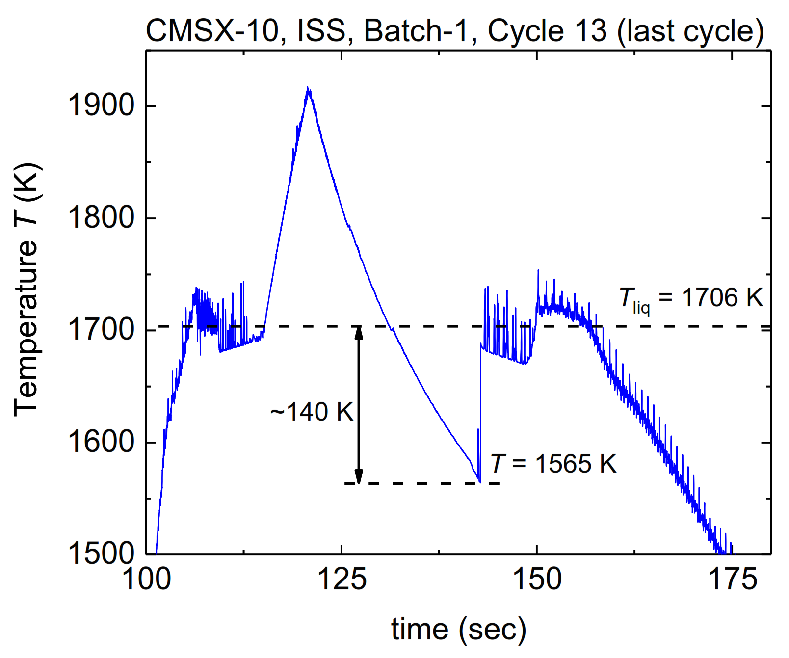
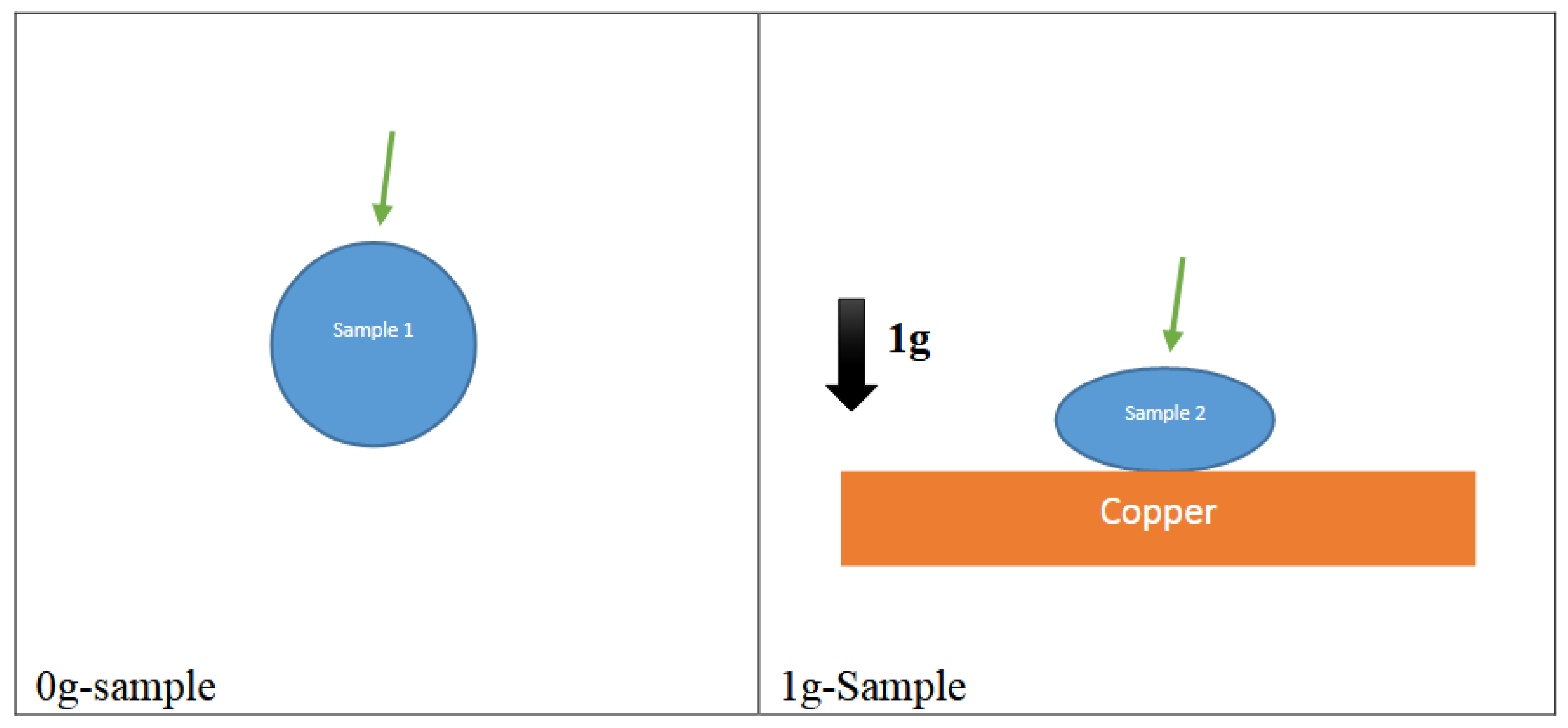
2.1. Short Experimental Review on the Differences in Solidification of CMSX-10 in 1g and 0g
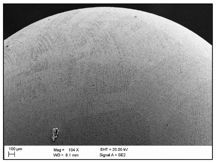
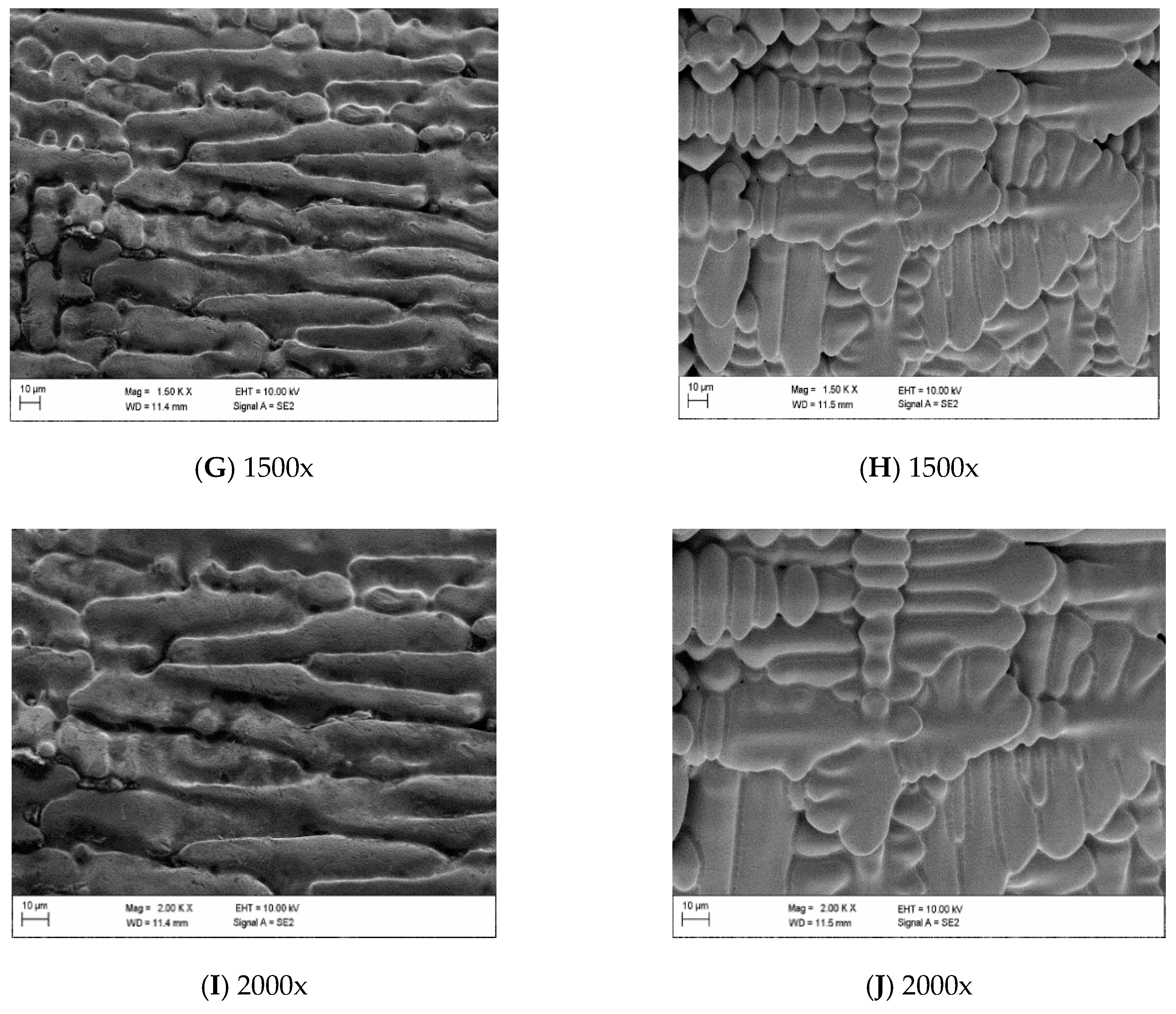
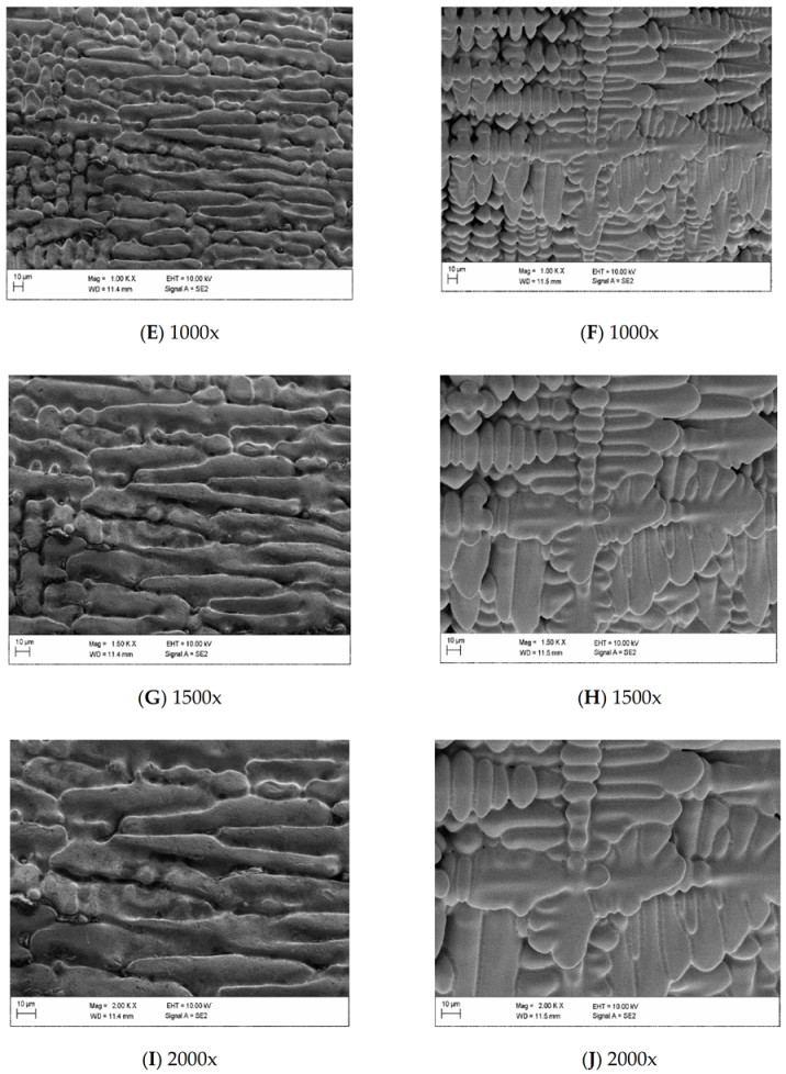
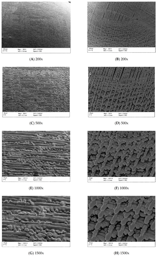
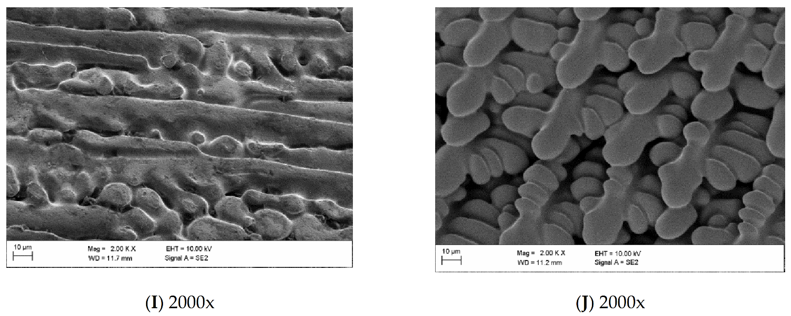
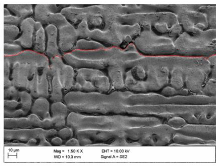
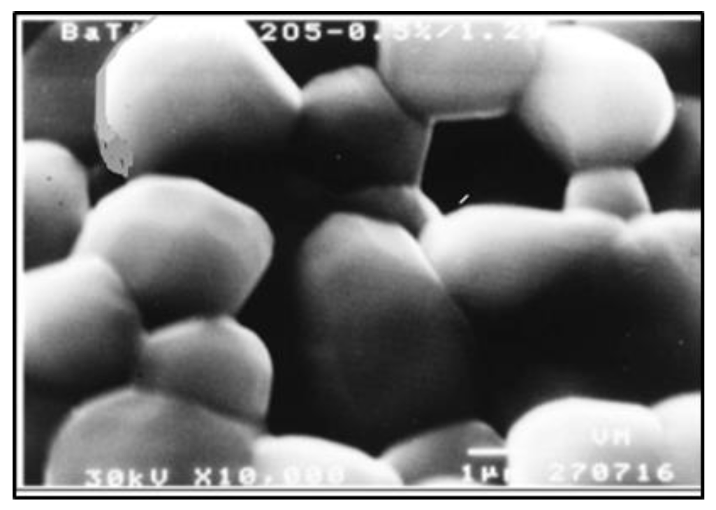
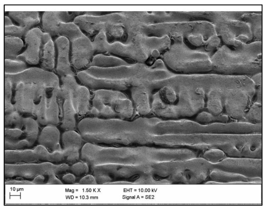
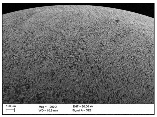
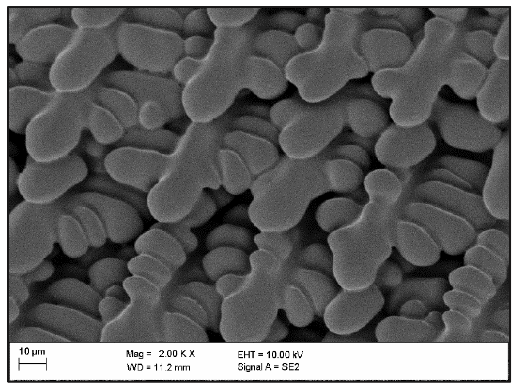
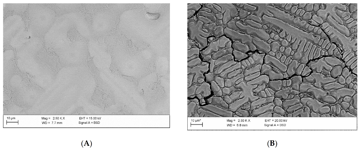
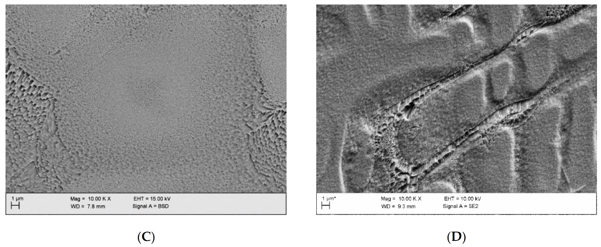
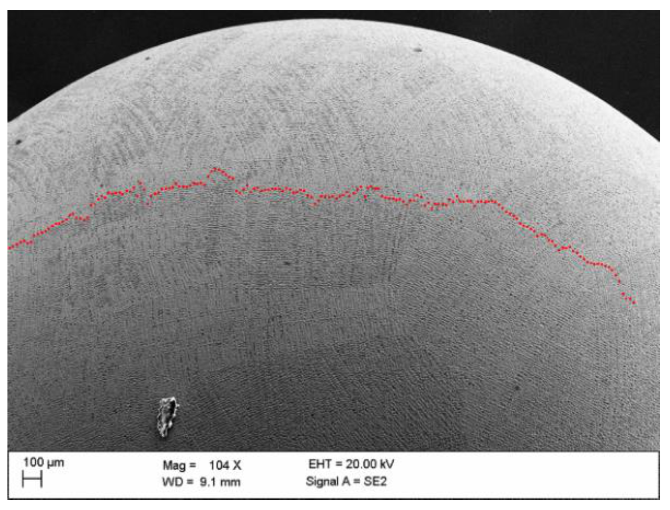
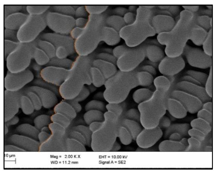
2.1.1. SEM Images of the Surface
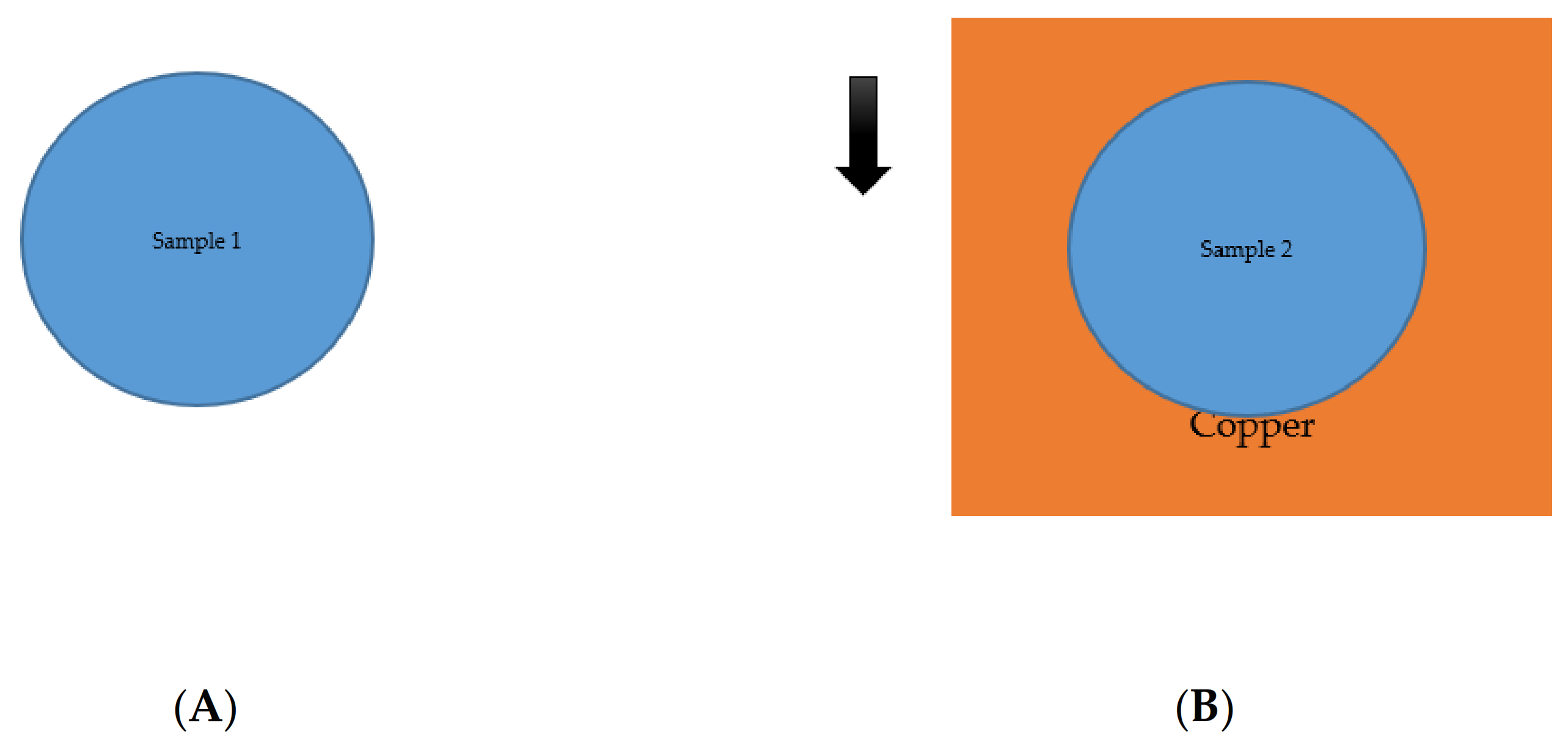
- CMSX-10–solidified onboard the ISS, “0g-Sample”
- CMSX-10–solidified on top of a water-cooled copper block, on the ground, in the Arc-Melter, “1g-Sample”
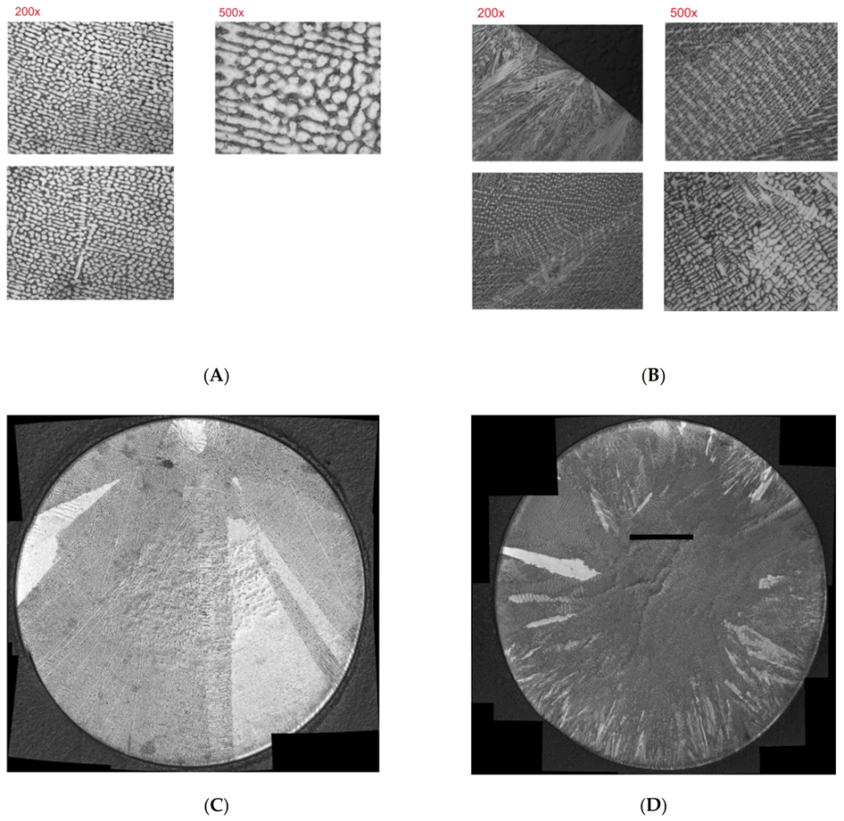
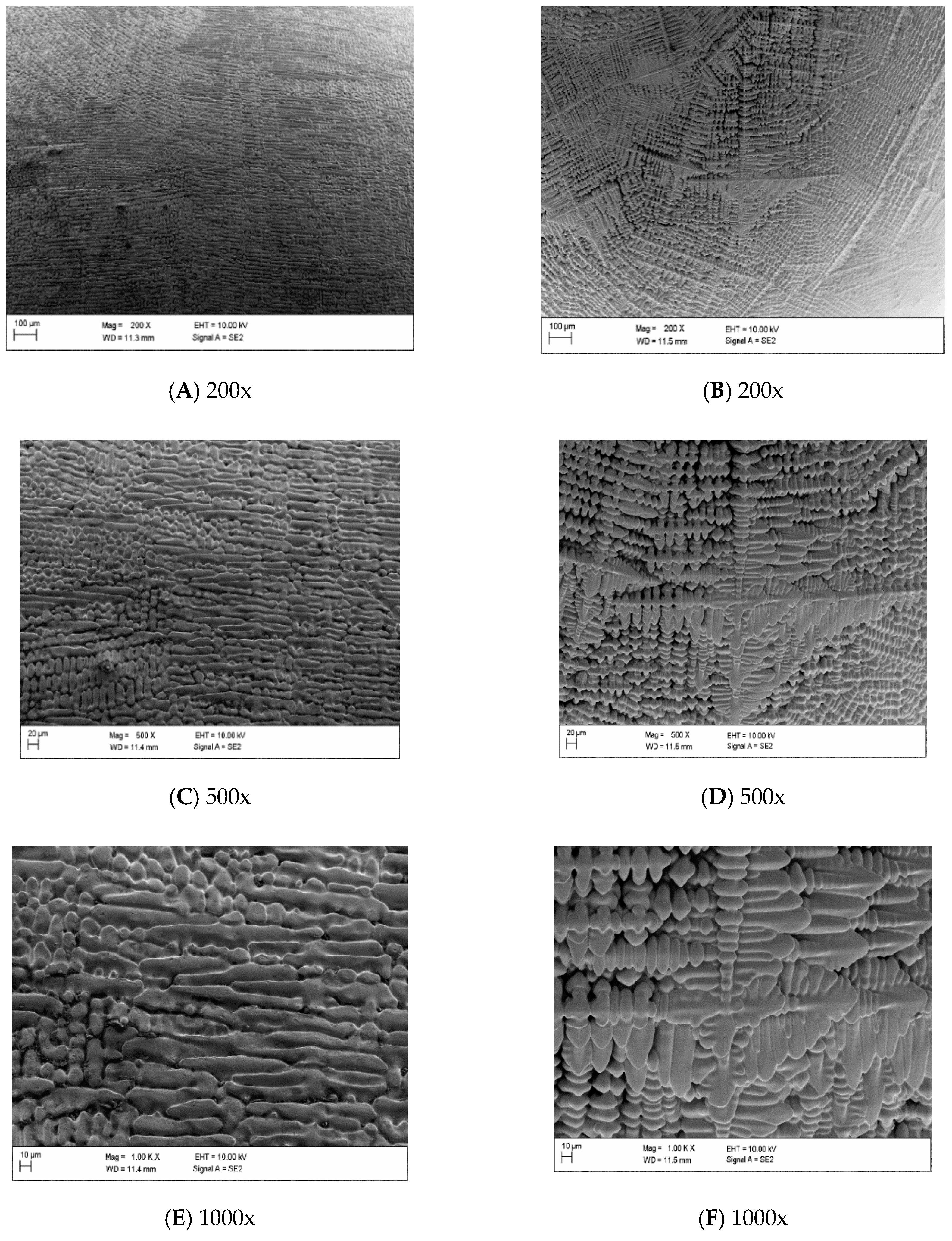
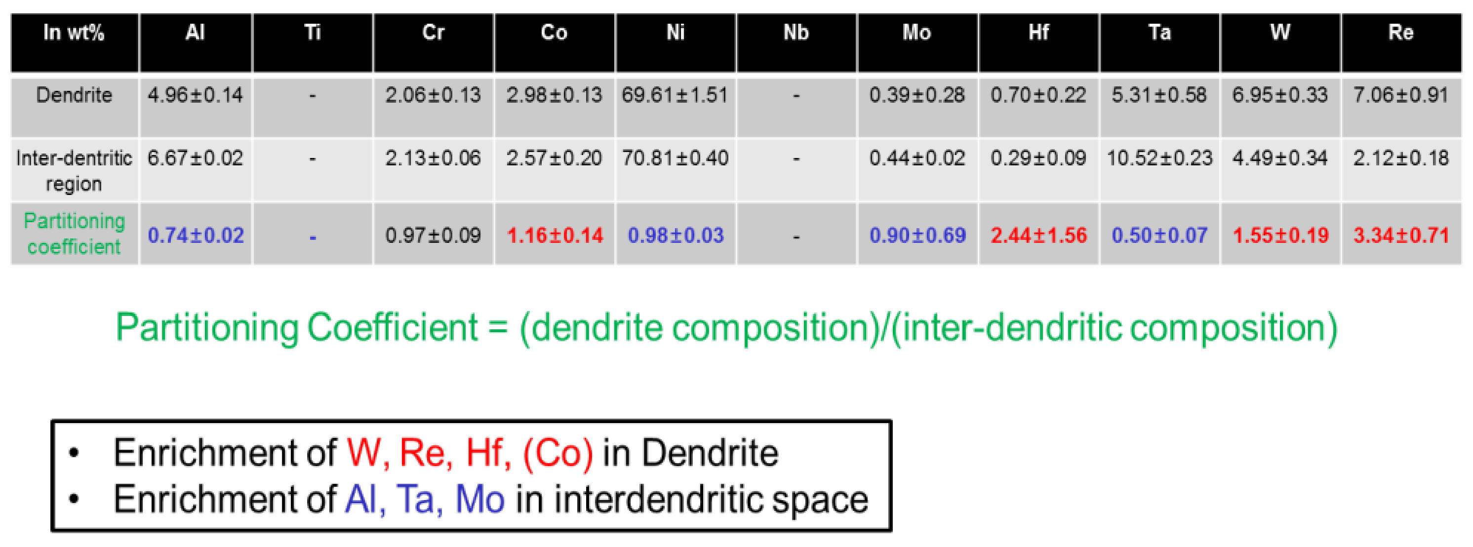
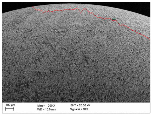
2.1.2. Images of Cross-Sections
- 3.
- CMSX-10–solidified onboard the ISS, “0g-Sample”.
- 4.
- CMSX-10–solidified by suction casting, on the ground, in the Arc-Melter, “1g-Sample”.
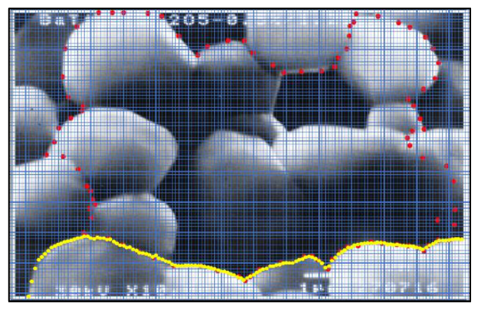
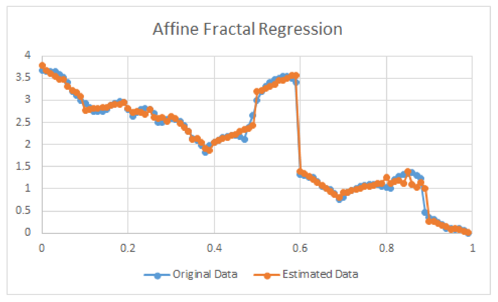
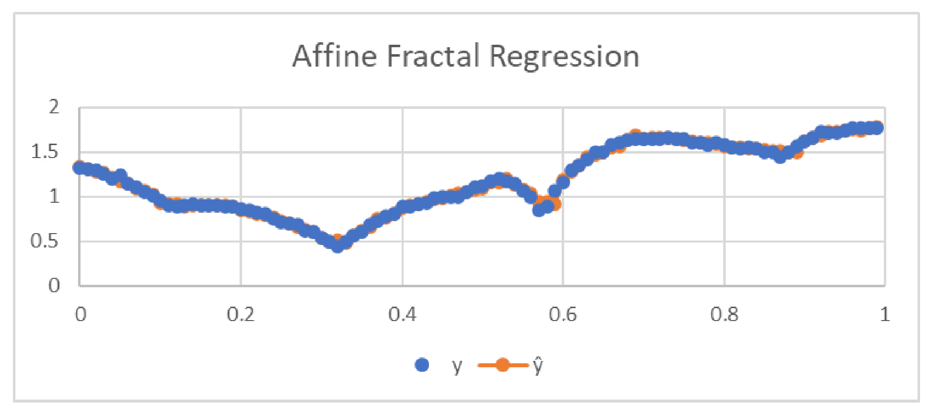
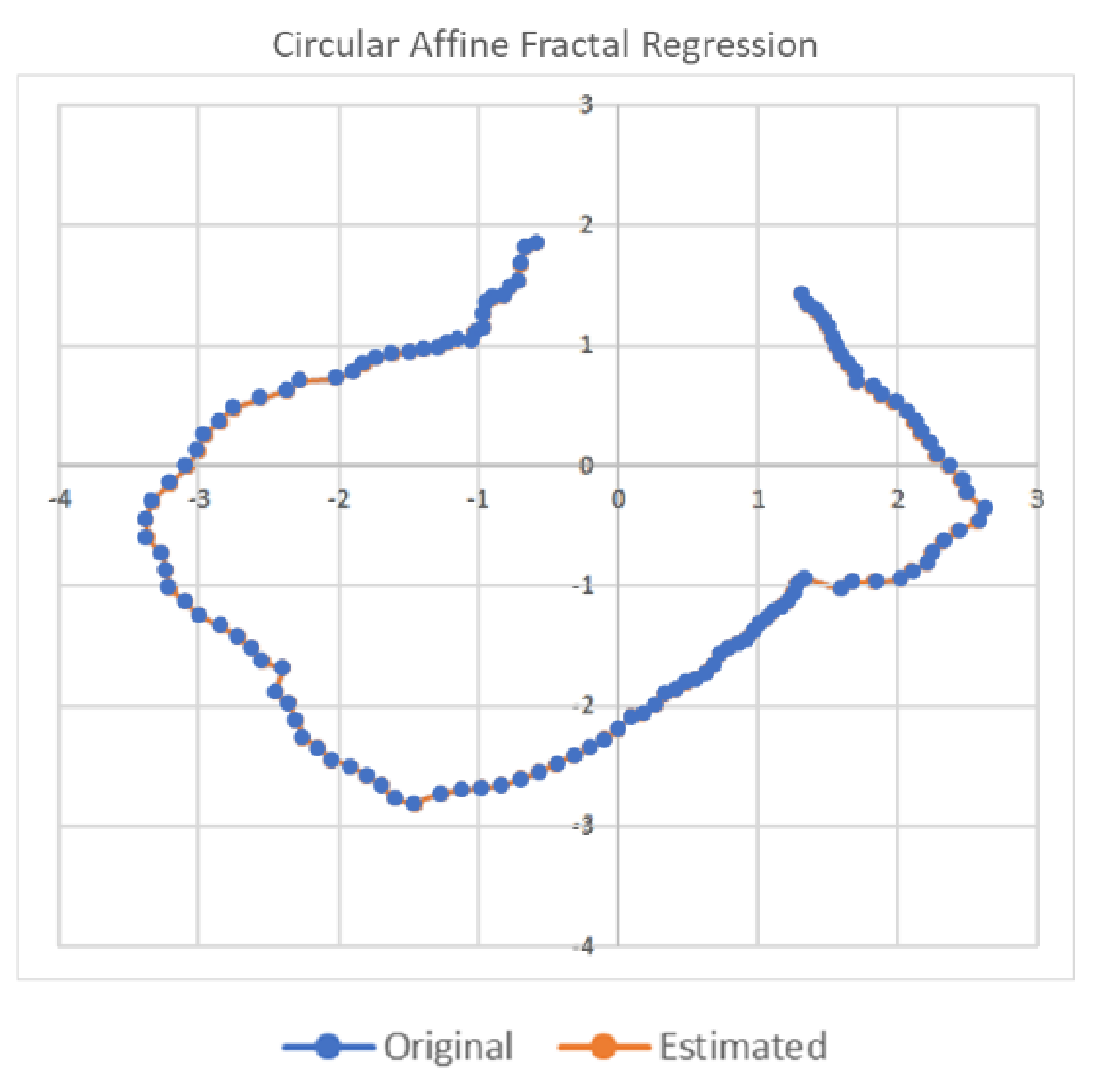
2.1.3. Mathematical Fractal Analysis Technique
3. Results
3.1. Comparison of the Surface Images
3.2. Comparison of the Cross-Section Images
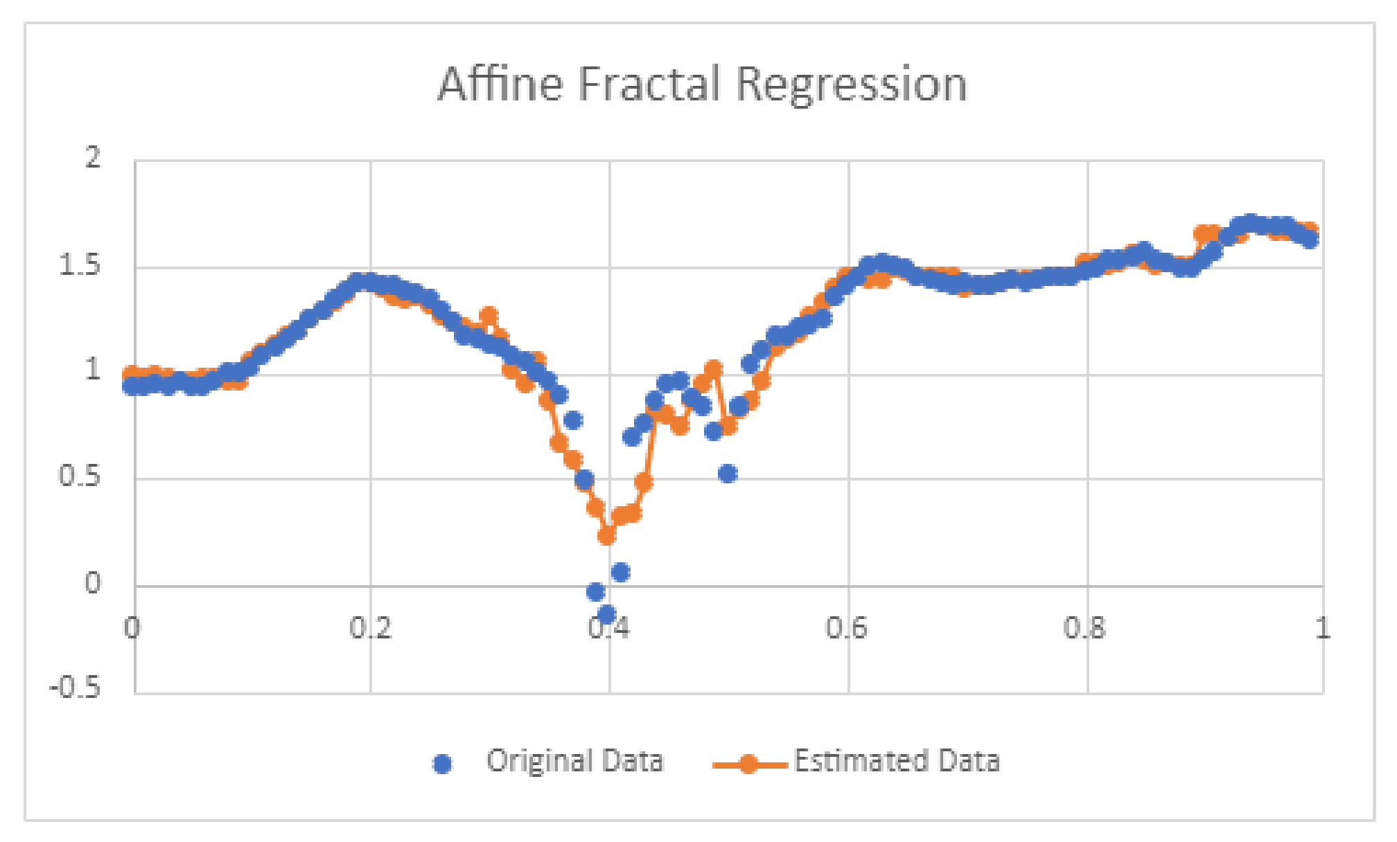
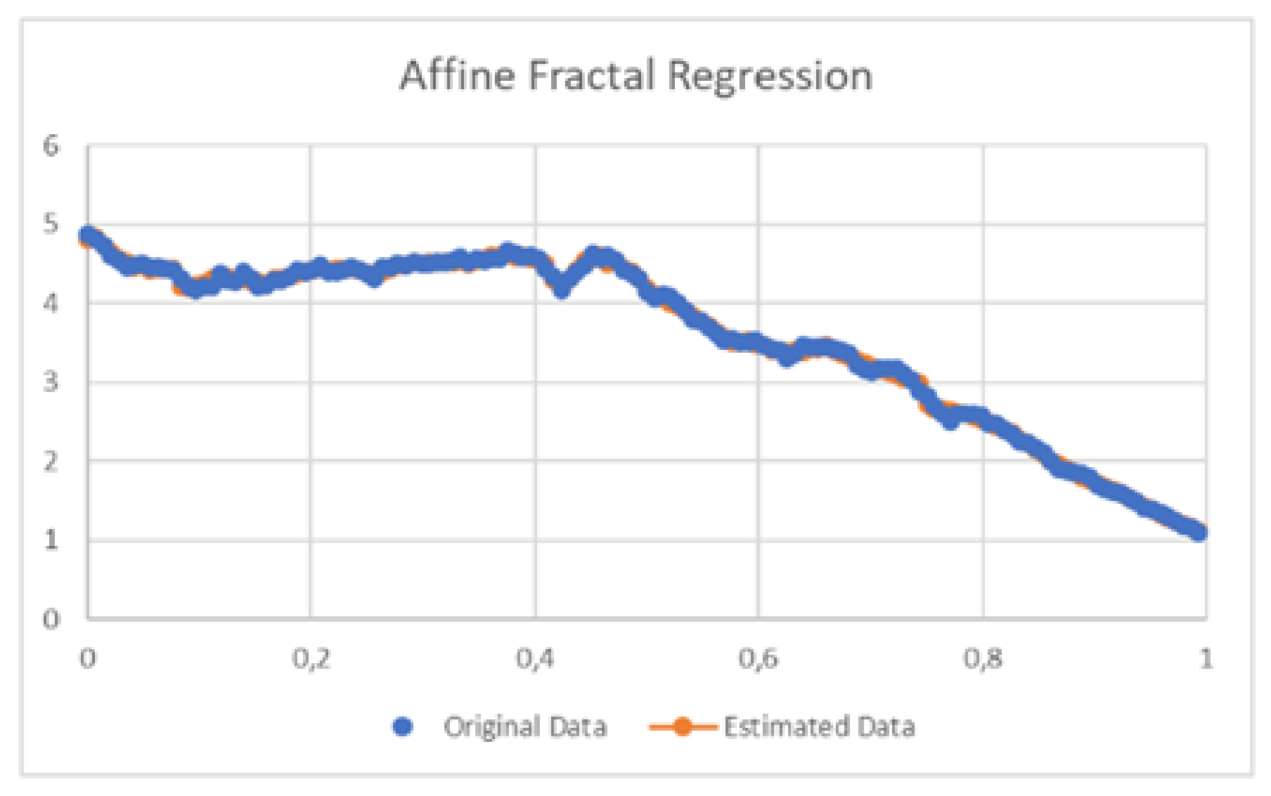
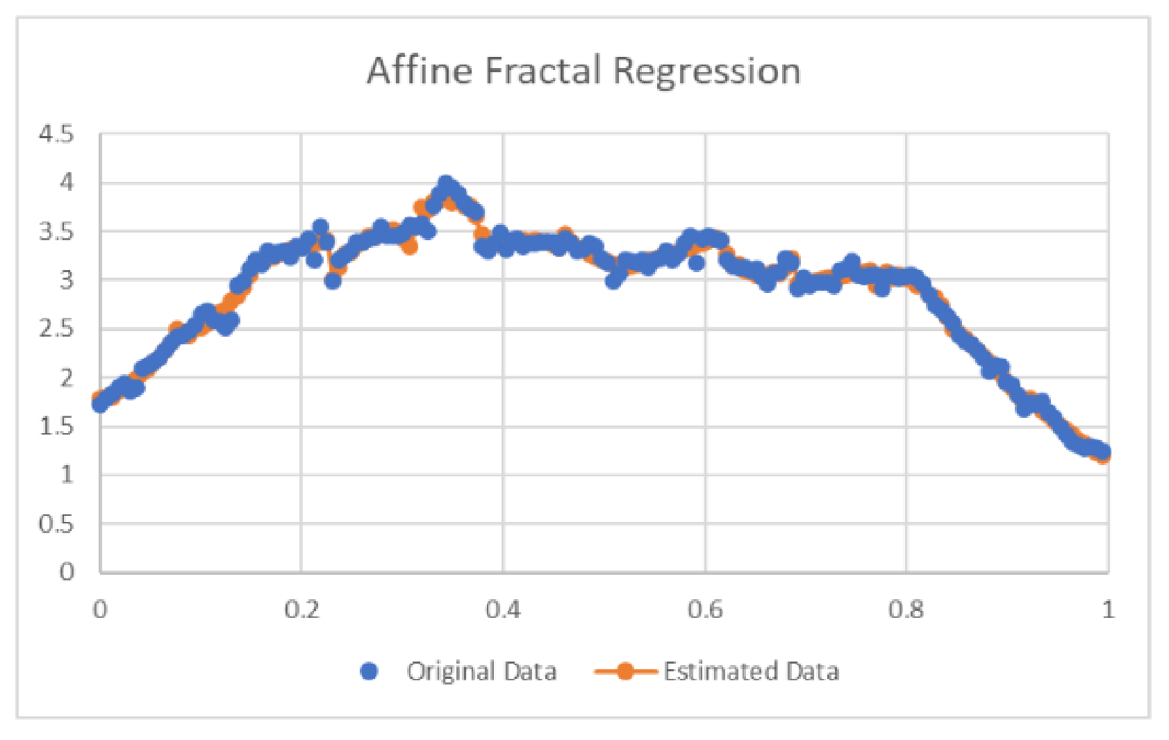
3.3. Fractal Analysis of the Images Consolidated in Space
3.4. Fractal Analysis of an Image Consolidated on Earth
4. Discussion
5. Conclusions
Author Contributions
Funding
Institutional Review Board Statement
Informed Consent Statement
Data Availability Statement
Acknowledgments
Conflicts of Interest
References
- Siauwand, T.; Bayen, A.M. An Introduction to MATLAB Programming and Numerical Methods for Engineers; Elsevier: Oxford/London, UK; Waltham, MA, USA; San Diego, CA, USA; Amsterdam, The Netherlands, 2015. [Google Scholar]
- Serpa, C.; Buescu, J. Constructive Solutions for Systems of Iterative Functional Equations. Constr. Approx. 2017, 45, 273–299. [Google Scholar] [CrossRef]
- Serpa, C.; Buescu, J. Explicitly defined fractal interpolation functions with variable parameters. Chaos Solitons Fractals 2015, 75, 76–83. [Google Scholar] [CrossRef]
- Buescu, J.; Serpa, C. Fractal and Hausdorff dimensions for systems of iterative functional equations. J. Math. Anal. Appl. 2019, 480, 1–19. [Google Scholar] [CrossRef]
- Barnsley, M.F. Fractal functions and interpolation. Constr. Approx. 1986, 2, 303–329. [Google Scholar] [CrossRef]
- Kenney, J.F.; Keeping, E.S. Linear Regression and Correlation, Ch. 15. In Mathematics of Statistics, 3rd ed.; Van Nostrand: Princeton, NJ, USA, 1962; pp. 252–285. [Google Scholar]
- Terner, M.; Yoon, H.Y.; Hong, H.U.; Seo, S.M.; Gu, J.H.; Lee, J.H. Clear path to the directional solidification of Ni-based superalloy CMSX-10: A peritectic reaction. Mater. Charact. 2015, 105, 56–63. [Google Scholar] [CrossRef]
- Wilson, B.C.; Cutler, E.R.; Fuchs, G.E. Effect of solidification parameters on the microstructures and properties of CMSX-10. Mater. Sci. Eng. A 2008, 479, 356–364. [Google Scholar] [CrossRef]
- Mohr, M.; Furrer, D.; Fecht, H. Thermophysical Properties of Advanced Ni-Based Superalloys in the Liquid State Measured on Board the International Space Station. Adv. Eng. Mater. 2020, 22, 1901228. [Google Scholar] [CrossRef]
- Mitić, V.; Goran, L.; Vesna, P.; Hwu, J.R.; Tsay, S.C.; Perng, T.P.; Sandra, V.; Branislav, V. Ceramic materials and energy-Extended Coble’s model and fractal nature. J. Eur. Ceram. Soc. 2019, 39, 3513–3525. [Google Scholar] [CrossRef]
- Mandelbrot, B. The Fractal Geometry of Nature; W. H. Freeman: New York, NY, USA, 1977. [Google Scholar]
- Arnold, W.; Fischer, H.-H.; Knapmeyer, M.; Krüger, H. Surface Mechanical Properties of Comet 67P. Jpn. J. Appl. Phys. 2019, 58, SG0801. [Google Scholar] [CrossRef]
- Mitić, V.; Kocić, L.J.M.; Mitrović, I.Z. Fractals in Ceramic Structure. In Proceedings of the IX World Round Table Conference on Sintering, Belgrade, Serbia, 1–4 September 1998; Advanced Science and Technology of Sintering. Stojanović, B.D., Skorokhod, V.V., Nikolić, M.V., Eds.; Kluwer Academic/Plenum Publishers: New York, NY, USA, 1999; pp. 397–402. [Google Scholar]
- Mitic, V.V.; Lazovic, G.; Mirjanic, D.; Fecht, H.; Vlahovic, B.; Arnold, W. The Fractal Nature as New Frontiers in Microstructure Characterization and Relativisation the Scale Sizes within the Space. Mod. Phys. Lett. B 2020, 34, 2050421. [Google Scholar] [CrossRef]


| Composition in wt% | CMSX-10 |
|---|---|
| Ni | Bal. |
| Al | 5.7 |
| Cr | 2.0 |
| Co | 3.0 |
| Mo | 0.4 |
| W | 5.0 |
| Ti | 0.2 |
| Re | 6.0 |
| Ta | 8.0 |
| Hf | 0.03 |
| Nb | 0.1 |
| 0 | 1 | 2 | 3 | 4 | 5 | 6 | 7 | 8 | 9 | |
|---|---|---|---|---|---|---|---|---|---|---|
| 0.018 | 0.011 | −0.046 | −0.175 | −0.229 | −0.073 | −0.044 | −0.006 | −0.038 | −0.051 | |
| −0.03 | 0.401 | −0.231 | −0.861 | 1.046 | 0.778 | 0.032 | 0.069 | 0.008 | 0.063 | |
| 0.967 | 1.043 | 1.47 | 1.437 | 0.46 | 0.824 | 1.494 | 1.41 | 1.566 | 1.699 |
| 0 | 1 | 2 | 3 | 4 | 5 | 6 | 7 | 8 | 9 | 10 | 11 | |
|---|---|---|---|---|---|---|---|---|---|---|---|---|
| −0.14 | 0.09 | 0.059 | 0.055 | 0.097 | 0.268 | 0.025 | −0.098 | −0.012 | 0.043 | −0.05 | −0.015 | |
| −0.89 | 0.324 | 0.318 | 0.348 | 0.291 | 0.941 | −0.651 | −0.398 | −0.49 | −0.254 | −0.813 | −0.607 | |
| 5.487 | 3.788 | 4.03 | 4.103 | 4.072 | 3.009 | 4.062 | 3.987 | 3.462 | 2.513 | 2.513 | 1.702 |
| 0 | 1 | 2 | 3 | 4 | 5 | 6 | 7 | 8 | 9 | 10 | 11 | 12 | |
|---|---|---|---|---|---|---|---|---|---|---|---|---|---|
| −0.051 | −0.105 | 0.01 | 0.141 | 0.272 | 0.042 | −0.066 | −0.018 | −0.158 | 0 | 0.133 | 0.028 | −0.026 | |
| 0.63 | 0.599 | 0.262 | 0.453 | 0.128 | 0.004 | −0.332 | 0.269 | −0.191 | 0.155 | −0.364 | −0.831 | −0.632 | |
| 1.873 | 2.685 | 3.155 | 2.75 | 2.862 | 3.257 | 3.587 | 3.226 | 3.683 | 0.955 | 2.713 | 2.447 | 1.835 |
| 0 | 1 | 2 | 3 | 4 | 5 | 6 | 7 | 8 | 9 | |
|---|---|---|---|---|---|---|---|---|---|---|
| 0.051 | −0.025 | 0.092 | −0.07 | −0.017 | 0.037 | −0.001 | 0.025 | 0.192 | −0.026 | |
| −0.58 | 0.101 | 0.032 | −1.117 | 0.351 | 0.561 | −0.653 | 0.334 | 0.462 | −0.374 | |
| 3.588 | 2.859 | 2.474 | 2.899 | 2.111 | 3.057 | 1.407 | 0.818 | 0.544 | 0.363 |
| 0 | 1 | 2 | 3 | 4 | 5 | 6 | 7 | 8 | 9 | 10 | |
|---|---|---|---|---|---|---|---|---|---|---|---|
| −0.079 | −0.038 | 0.071 | 0.06 | 0.051 | 0.015 | −0.035 | −0.023 | 0.075 | −0.033 | −0.023 | |
| −0.488 | 0.733 | 1.136 | −0.534 | 0.087 | −0.904 | −0.419 | −0.095 | 0.843 | −0.619 | 0.1 | |
| 2.102 | 1.552 | 2.247 | 3.309 | 2.994 | 2.979 | 2.158 | 1.751 | 1.742 | 2.566 | 1.891 |
Publisher’s Note: MDPI stays neutral with regard to jurisdictional claims in published maps and institutional affiliations. |
© 2021 by the authors. Licensee MDPI, Basel, Switzerland. This article is an open access article distributed under the terms and conditions of the Creative Commons Attribution (CC BY) license (https://creativecommons.org/licenses/by/4.0/).
Share and Cite
Mitić, V.; Serpa, C.; Ilić, I.; Mohr, M.; Fecht, H.-J. Fractal Nature of Advanced Ni-Based Superalloys Solidified on Board the International Space Station. Remote Sens. 2021, 13, 1724. https://doi.org/10.3390/rs13091724
Mitić V, Serpa C, Ilić I, Mohr M, Fecht H-J. Fractal Nature of Advanced Ni-Based Superalloys Solidified on Board the International Space Station. Remote Sensing. 2021; 13(9):1724. https://doi.org/10.3390/rs13091724
Chicago/Turabian StyleMitić, Vojislav, Cristina Serpa, Ivana Ilić, Markus Mohr, and Hans-Jörg Fecht. 2021. "Fractal Nature of Advanced Ni-Based Superalloys Solidified on Board the International Space Station" Remote Sensing 13, no. 9: 1724. https://doi.org/10.3390/rs13091724
APA StyleMitić, V., Serpa, C., Ilić, I., Mohr, M., & Fecht, H.-J. (2021). Fractal Nature of Advanced Ni-Based Superalloys Solidified on Board the International Space Station. Remote Sensing, 13(9), 1724. https://doi.org/10.3390/rs13091724