The Sentinel-3 SLSTR Atmospheric Motion Vectors Product at EUMETSAT

Abstract

Atmospheric Motion Vectors (AMVs) are an important input to many Numerical Weather Prediction (NWP) models. EUMETSAT derives AMVs from several of its orbiting satellites, including the geostationary satellites (Meteosat), and its Low-Earth Orbit (LEO) satellites. The algorithm extracting the AMVs uses pairs or triplets of images, and tracks the motion of clouds or water vapour features from one image to another. Currently, EUMETSAT LEO satellite AMVs are retrieved from georeferenced images from the Advanced Very-High-Resolution Radiometer (AVHRR) on board the Metop satellites. EUMETSAT is currently preparing the operational release of an AMV product from the Sea and Land Surface Temperature Radiometer (SLSTR) on board the Sentinel-3 satellites. The main innovation in the processing, compared with AVHRR AMVs, lies in the co-registration of pairs of images: the images are first projected on an equal-area grid, before applying the AMV extraction algorithm. This approach has multiple advantages. First, individual pixels represent areas of equal sizes, which is crucial to ensure that the tracking is consistent throughout the processed image, and from one image to another. Second, this allows features that would otherwise leave the frame of the reference image to be tracked, thereby allowing more AMVs to be derived. Third, the same framework could be used for every LEO satellite, allowing an overall consistency of EUMETSAT AMV products. In this work, we present the results of this method for SLSTR by comparing the AMVs to the forecast model. We validate our results against AMVs currently derived from AVHRR and the Spinning Enhanced Visible and InfraRed Imager (SEVIRI). The release of the operational SLSTR AMV product is expected in 2022.

1. Introduction

In the field of wind observations, Atmospheric Motion Vectors (AMVs) prevail as a globally available, mesoscale measurement of winds. AMVs are routinely assimilated in Numerical Weather Prediction (NWP), where they have a significant positive impact on weather forecasting and nowcasting [1,2,3]. EUMETSAT already derives AMVs from its Meteosat Second Generation (MSG) satellites, Meteosat-11 at 0° East, Meteosat-10 at $9.5$° East in rapid scan mode and Meteosat-8 at $41.5$° East, and from its Low-Earth Orbit (LEO) satellites, Metop A, B and C. AMV producers like EUMETSAT are always encouraged by end-users to propose AMV products from new sensors, to increase the coverage and density of wind observations. In particular, LEO satellite sensors allow observing atmospheric motion at high latitudes, which are not visible for geostationary satellite sensors [4,5]. Since the launch of Sentinel-3A (S3A) in 2016 and Sentinel-3B (S3B) in 2018, the Sea and Land Surface Temperature Radiometer (SLSTR) represents a viable new opportunity to derive AMVs in these critical areas. AMVs are derived from pairs of images from satellite sensors, by tracking clouds, or water vapour features, from one image to the other. Such tracking is easily achieved for sensors on board geostationary satellites, considering that successive images are co-registered spatially, have the same ground resolution and the time gap between images is small [6]. The situation is different for LEO satellites. Indeed, the time gap between successive overpasses is much higher, either 101 min (time needed to complete one orbit of Metop or Sentinel-3), or less when using images from different satellites. Not only does this increased time gap make the tracking of features from one image to another harder, but it also limits the derivation of AMVs to the area of overlap between the images. Additionally, the ground resolution of pixels varies depending on the viewing angle: pixels at nadir usually represent areas of about 1 km × 1 km each for SLSTR, while pixels at the border of the swath can represent areas as large as 5 km × 5 km each. The current implementation of AMV computation from EPS-Advanced Very-High-Resolution Radiometer (AVHRR) [7] consists in locating pixels of the second image inside the first image using their geographical coordinates, and then interpolate to fill the gaps between remapped pixels. The AMV derivation methodology we use for SLSTR is a slightly modified version of that used for AVHRR. In the following, we present this methodology, used to derive AMVs from images from band S8 (centred at 10,854 nm) of SLSTR. In Section 2, we present the input data and the algorithm used to derive AMVs, and give details about the final product. In Section 3, we give an overview of the performance of the SLSTR AMVs, by comparing them to ECMWF forecast model winds, MSG - Spinning Enhanced Visible and InfraRed Imager (SEVIRI) AMVs, and AVHRR AMVs.

2. Algorithm and Product Description

2.1. Input Data

2.1.1. Level-1B Data

The derivation of AMVs is based on SLSTR Level 1B (L1B) products. L1B products are available in the form of Product Dissemination Units (PDUs) of 2 or 3 min of data. Every orbit allows the production of 33 PDUs of 3 min and one PDU of 2 min, resulting in 484–485 PDUs per day. Currently, only the thermal infrared band of SLSTR, the band S8, centred at 10.854 micrometres, is used to derive AMVs. The L1B S8 data is disseminated in the form of Brightness Temperatures (BT), which are used by the AMV algorithm for the height assignment. However, features are tracked using the radiance images. Any pixels declared clouds by any masks within the L1B product are considered clouds in the AMV processing here. This permissive choice ensures the derivation of as many AMVs as possible, with the risk of sometimes deriving ground-level null vectors which should not be interpreted as movements.

2.1.2. Difference between S3A and S3B Products

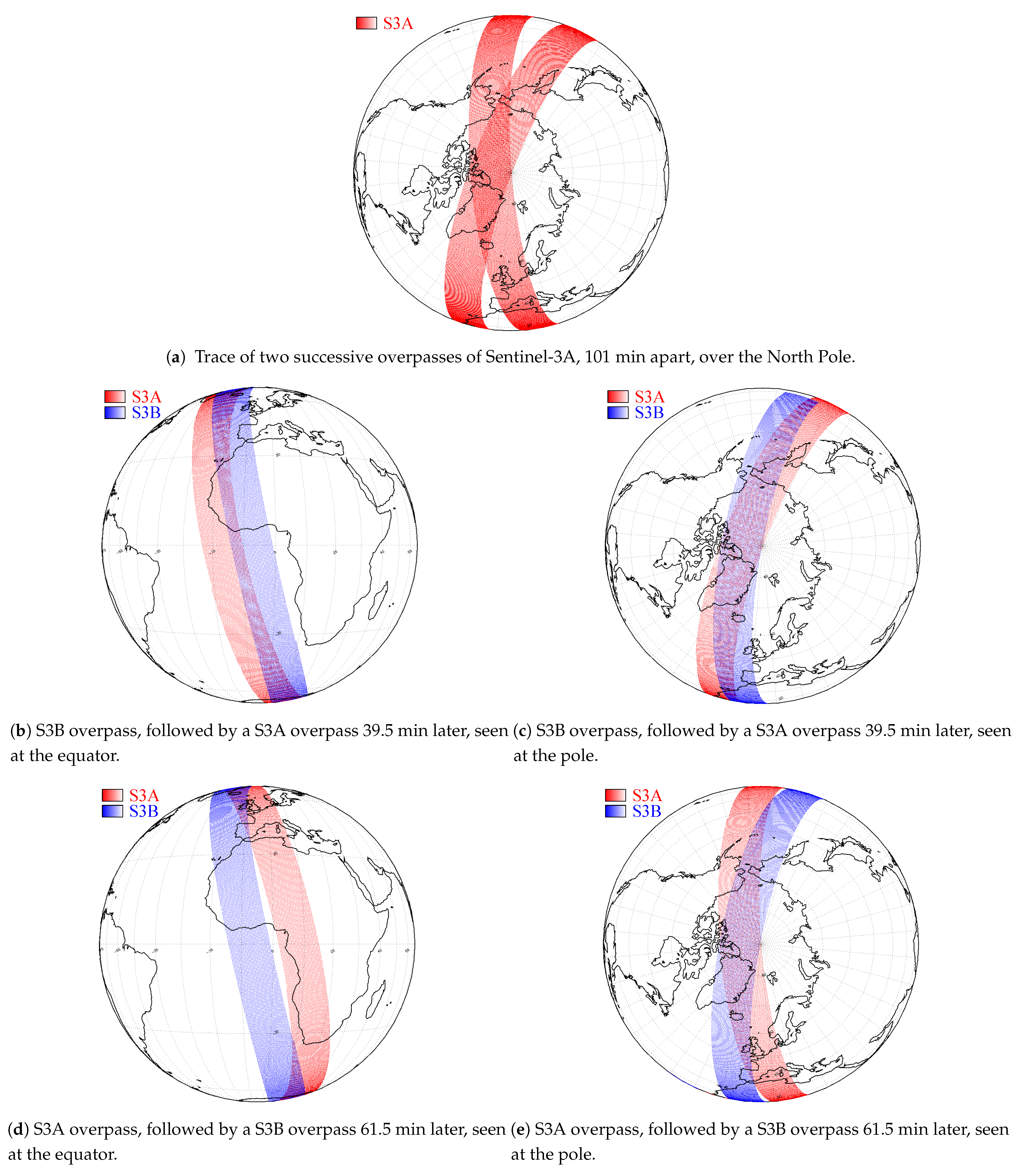
SLSTR AMVs are derived using L1B data from both Sentinel-3 satellites, S3A and S3B. The orbits of S3A and S3B are identical, but S3B flies 140 degrees out of phase with S3A. The 1420 km swath width of SLSTR has little overlap between successive overpasses of the same satellite (see Figure 1a). Furthermore, the temporal resolution of the observations is lower in a single platform approach (101 min) compared to a dual-platform approach (61.5 min or 39.5 min). Consequently, only dual-satellite (S3A and S3B combined) products will be disseminated.

The SLSTR AMV product consists of two complementary products from the S3A and S3B processing chains, even if both satellites data are used in both cases. The S3A (also called dual S3A/S3B) product considers S3A data as the reference image, and tracks the features backwards in S3B data (earlier pass), the second image; and conversely for the pair S3B/S3A. The phase between the two Sentinel-3 satellites implies a difference in the acquisition time gap for the two dual products: 39.5 min for S3A products, and 61.5 min for S3B products. This difference has three main consequences.

• S3A products cover all the globe, while S3B products are restricted to latitudes polewards of 50° (see Figure 1).
• S3A allows the production of many more AMVs than S3B. According to our study, about twice as many AMVs are derived from S3A as from S3B (see Section 3).
• The quality of AMVs, relative to the ECMWF forecast model, is higher for S3B than for S3A (as explained in Section 3).

2.2. Projection of Scans

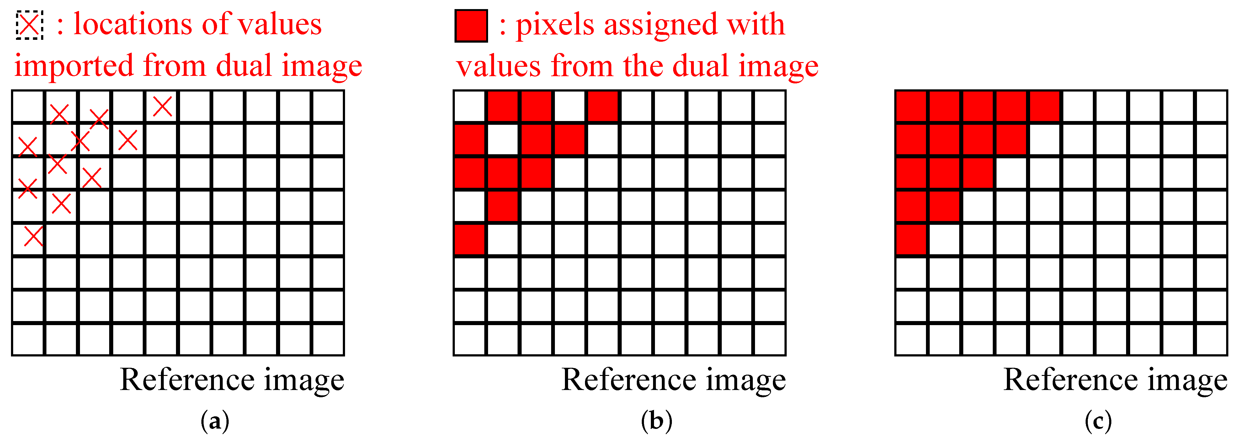
The main difference between the processing of SLSTR AMVs and that of AVHRR AMVs is the co-registration of the images, prior to the derivation of AMVs. Currently, pairs of AVHRR L1B images are co-registered by mapping the second image on the reference image. Values are assigned to the nearest neighbouring pixels, and then interpolated with a 2D bilinear interpolation (see Figure 2).

The approach described above has several drawbacks.

• Depending on the viewing angle, pixels of the reference frame may represent areas from 1 km × 1 km to 5 km × 5 km. The varying spatial resolution over the images induces a scale factor effect, possibly resulting in tracking inconsistency.
• The tracking is limited to the frame of the reference image. Clouds in both images which moved from outside of the frame (in the second image) to the inside of the frame cannot be tracked.
• This approach uses only one PDU from each orbit. However, successive SLSTR scans may be put in different PDUs, resulting in the loss of potential features lying in these scans.

For all these reasons, another methodology is used to co-register SLSTR data: L1B scans are projected onto an equal-area grid (see Figure 3).

EUMETSAT developped a Generic Projection Tool [8] based on the ground track oblique Cassini projection proposed by Mills [9] for VIIRS data. This tool is generic and can be used for all other LEO satellites like the future EPS-SG/METimage at EUMETSAT. The projection solves the aforementioned problems: it ensures a constant ground resolution over both images; it makes it possible to track features leaving either image frame; and by projecting successive PDUs together on the same grid, features lying at the edges of the reference image may be tracked. All these new elements together allow deriving many more AMVs, and a more consistent tracking across the images. The resolution of the projection, for the operational product to come, is set to 1 km, the nominal spatial resolution at the nadir of the thermal channel of SLSTR. The pixel field-of-view degrades down to almost 5 km on the edges of the swath. This means that a bilinear interpolation is necessary to achieve a constant ground resolution over all the image. In practice, this interpolation makes the features on the sides of the swath blurry, when compared to features at the centre. However, using the wind guess (see Section 2.3.2) allows the derivation of AMVs of acceptable quality, no matter the native ground resolution (as explained in Section 3.2). For this reason, the finest native ground resolution, 1 km, is preferred to other projection resolutions, which give fewer AMVs, although of marginally better quality.

2.3. Core AMV Algorithm

2.3.1. Target Selection

From here on, the algorithm is similar to those used for all other sensors utilised at EUMETSAT, including EPS-AVHRR and MSG-SEVIRI. The reference frame is divided into a regular grid of cells of 24 pixels. For each of these cells, we define a 32-pixel sized window, with the same centre as the cell. Within this window, the algorithm screens every frame of $24\times 24$ pixels in search of the one with highest contrast. To be selected as a target, the frame must meet the following criteria.

• At least 25 % of the target’s pixels shall be cloudy. Whether a pixel is cloudy is determined by the cloud mask available in the L1B product.
• Have a stricly positive contrast.
• The whole target lies in the frame of the reference image.
• The whole search area (as defined in Section 2.3.2) lies in the trace of the second image.

The selection of a target leads to the derivation of an AMV, unless the final correlation found with the matching target, at the motion tracking step, is below a given threshold.

2.3.2. Motion Tracking

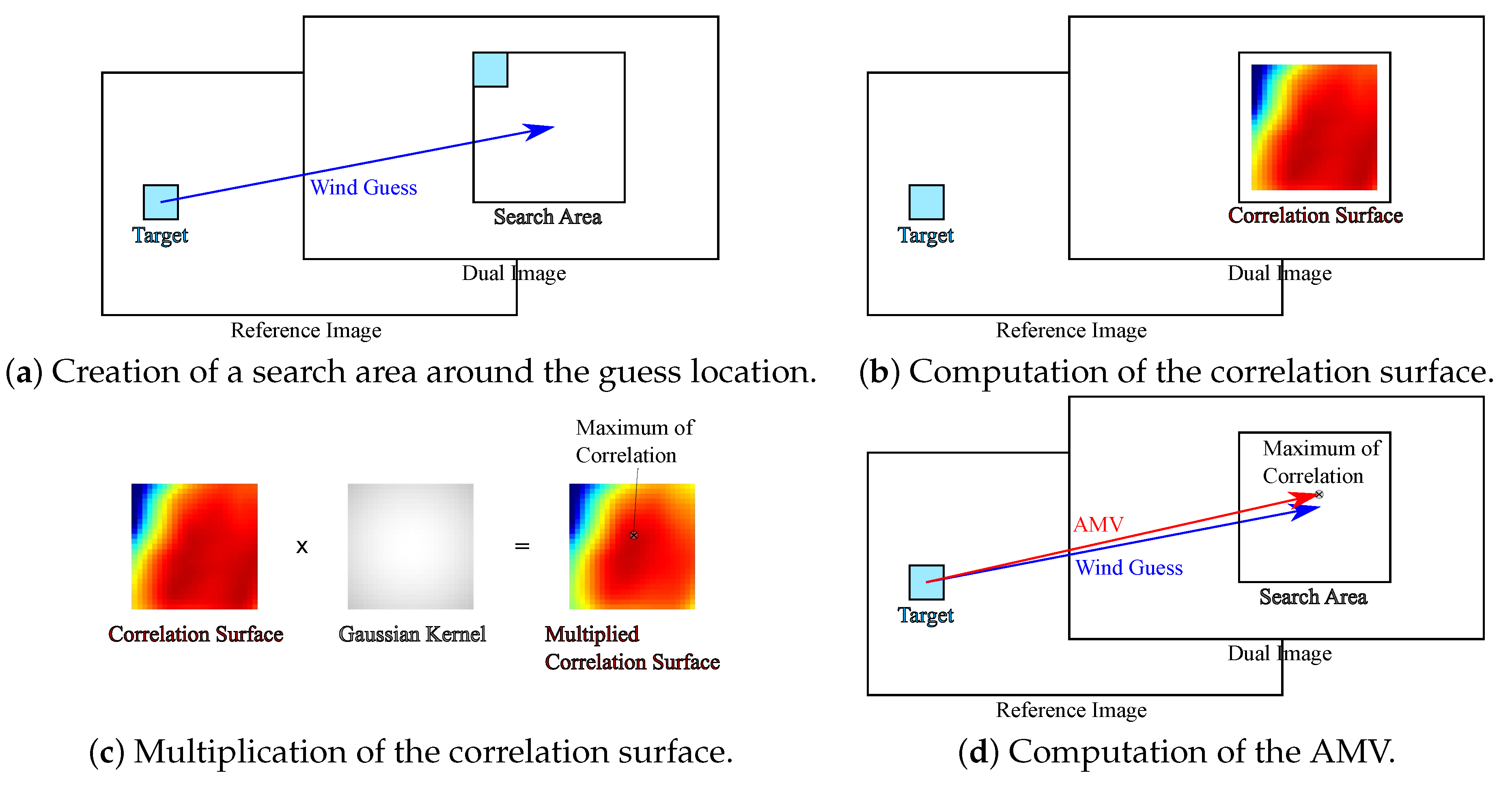
The tracking is performed backwards, that is, from the reference image to the dual image. Given the significant time gap between images for LEO satellites, a first guess is computed from wind forecasts to locate the search area’s position. It reduces computing time drastically and improves the robustness of AMV tracking. The impacts of the use of the guess are explained by Borde et Garcia Pereda [10]. The forecasted wind is retrieved at the location of the centre of the target, and at the height where the atmospheric temperature equals the average brightness temperature of the 20 % coldest pixels in the target. This rough estimation of the cloud height is also applied to AVHRR data [11]. We limit the search of a matching target to a search area of size $100\times 100$ pixels around the guessed feature location in the dual image. The cross-correlation between the starting target and the search area is computed, producing a correlation surface. The size of the search area relies on the expected error on the forecast wind. Since the time gap between the images varies among the AMV products, that size should also vary. This capability was introduced in the AVHRR AMV processing by the multiplication of the correlation surface with a Gaussian kernel. The objective is to maintain consistent quality between the two S3A and S3B products while decreasing the likelihood of deriving an outlier AMV. Consider $(x,y)$ the coordinates of a pixel in the correlation surface, $(0,0)$ being its centre, v the speed (in m/s) of the guess vector, $\Delta t$ the time gap between the acquisitions of the images (in seconds) and r the spatial resolution of the projection (in metres), then $g(x,y)$, the Gaussian weight at $(x,y)$ is given by Equation (1).

$$g(x,y)=exp\left(-{\left(\frac{\sqrt{x^2+y^2}}{\left(a\times v+b\right)\frac{\Delta t}{r}}\right)}^c\right)$$

(1)

In Equation (1), the parameters a, b and c can be adjusted depending on the confidence put in the forecast model. For the operational product, the values are $a=0.5$, $b=10$ m/s and $c=2$. The maximum of the multiplied correlation surface defines the centre of the matching target. This approach is summarised in Figure 4.

2.3.3. Height Assignment

The height assignment is based on the Cross-Correlation Contribution (CCC) method [12]. Basically, pixels that contribute the most to the final cross-correlation of the matched targets are selected, and the temperature used for the height assignment is the weighted mean of the temperatures of these pixels, the weights being the cross-correlation contributions. This temperature is placed in the ECMWF temperature profile, and the corresponding height is assigned to the AMV. Profiles are checked for temperature inversion and tropopause before assignment.

2.4. Final Product

The products will be disseminated in BUFR format [13], following the standard sequence 3-10-077. The satellite identifier for the SLSTR AMV product is coded 856, “combination of Sentinel-3 satellites”.

Up to one AMV product per L1B PDU can be derived, depending on the overlap and the cloudiness. In the offline data in production at EUMETSAT since June 2020, actual numbers of products are on average 480 per day for S3A, and 280 per day for S3B. Indeed, the two products are asymmetric, as explained in Section 2.1.2.

3. Results and Validation

3.1. Comparison to ECMWF Forecast Data

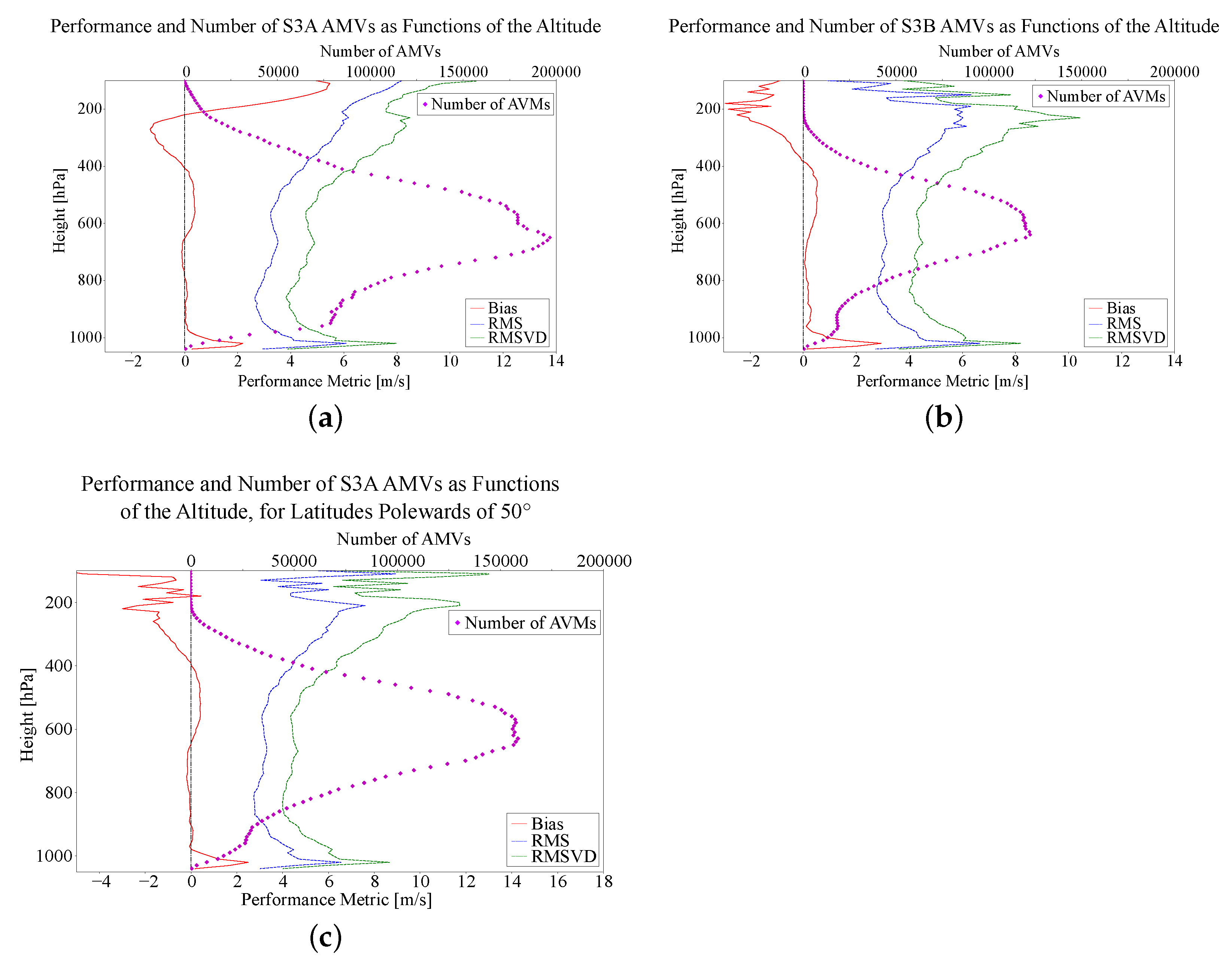
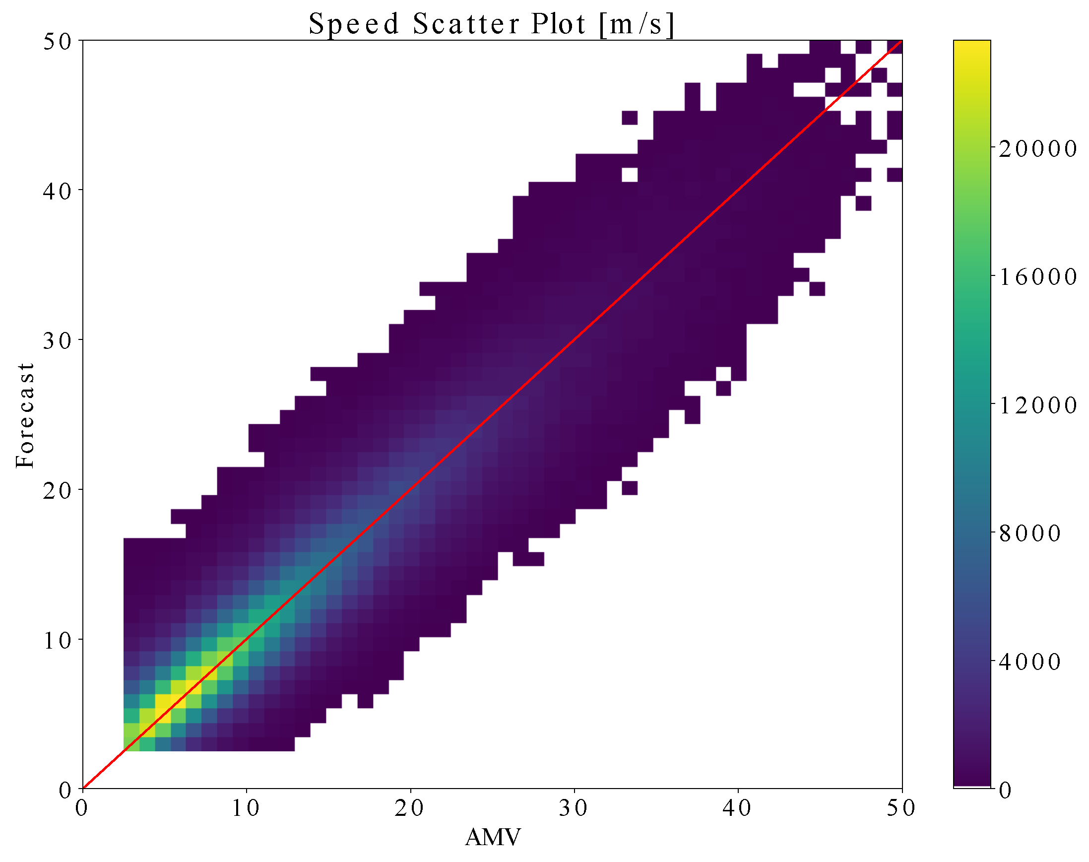
Our AMV data are first checked against the ECMWF forecast model. The forecast is available in the form of GRIB files with a 3-h step. We interpolate this information spatially (in height and planar location) and temporally to get the forecasted wind vector at the location and time of the AMV. We study here one month of SLSTR AMV data, 15 December 2020 to 15 January 2021. Several statistics and plots are shown here to illustrate the comparison. First, we show the scatter plots of AMVs speeds against co-located forecast wind speeds, Figure 5. Second, we plot the biases, Root Mean Square (RMS) errors and Root Mean Square Vector Differences (RMSVD) of AMVs against forecast as functions of the altitude, Figure 6. Third, we report a series of statistics, including RMS error on the speeds, RMSVD, overall biases, and numbers of AVMs derived,

Table 1. Statistics relative to SLSTR AMVs derived during the period of 15 December 2020–15 January 2021.

	S3A	S3A	S3B	S3A	S3A	S3B
	All AMVs	AMVs	All AMVs	Speed	AMVs	Speed
		Polewards		>2.5 m/s,	Polewards	>2.5 m/s,
		of 50°		QI > 60	of 50°,	QI > 60
					Speed > 2.5 m/s,
					QI > 60
RMS [m/s]	4.90	4.96	4.57	3.60	3.46	3.27
RMSVD [m/s]	6.50	6.30	5.96	5.06	4.86	4.65
Bias [m/s]	−0.46	−0.96	−0.56	0.08	0.12	0.29
Number of AMVs	16,929,930	11,399,723	9,320,270	9,158,914	6,491,511	4,730,554

. Statistics are reported for two sets of data: the full set, and the set of good quality AMVs, conventionally defined (for LEO satellites) as the AMVs faster than 2.5 m/s and of Quality Index (QI) [14] above 60 among the wind scientific community.

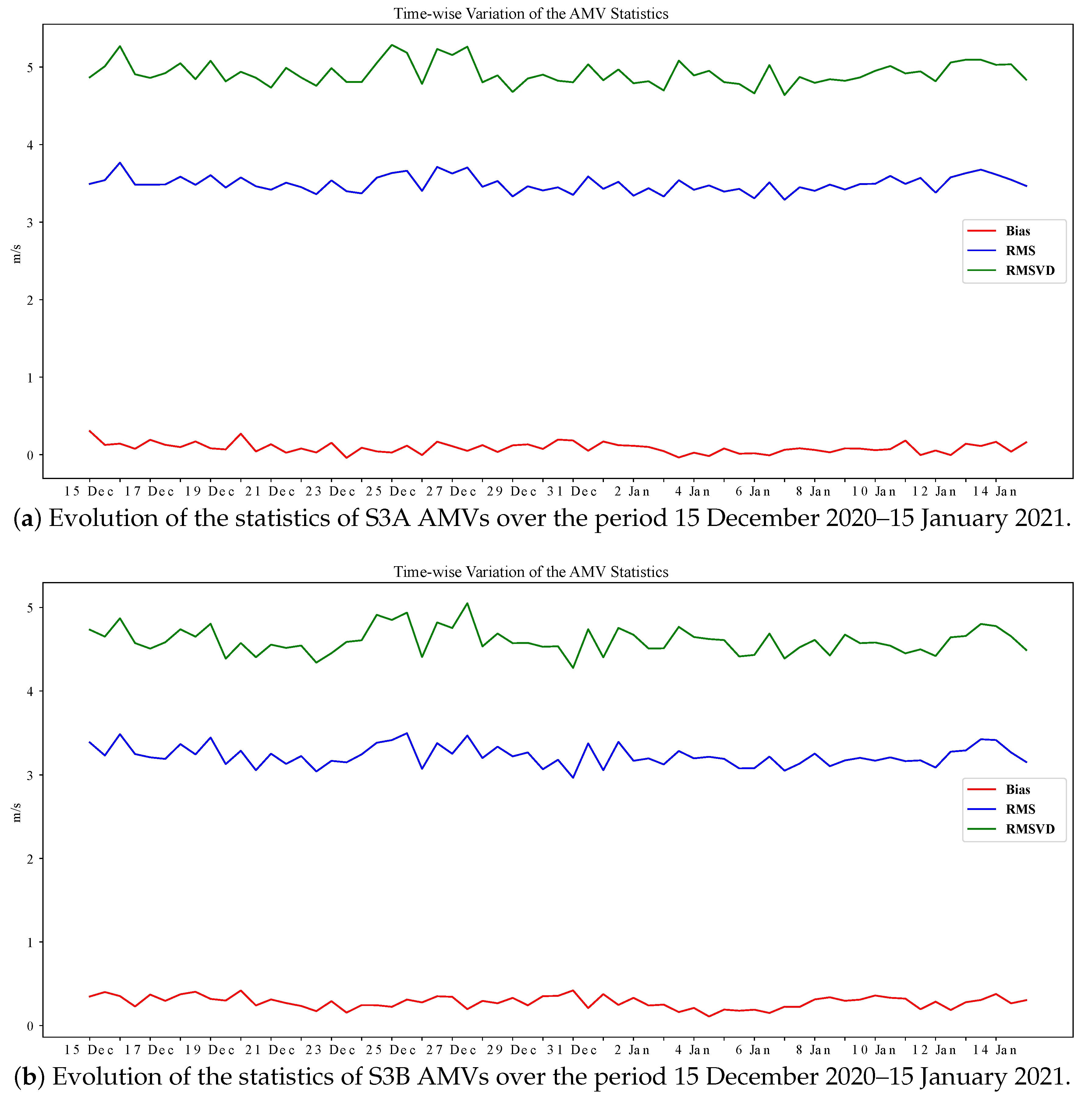
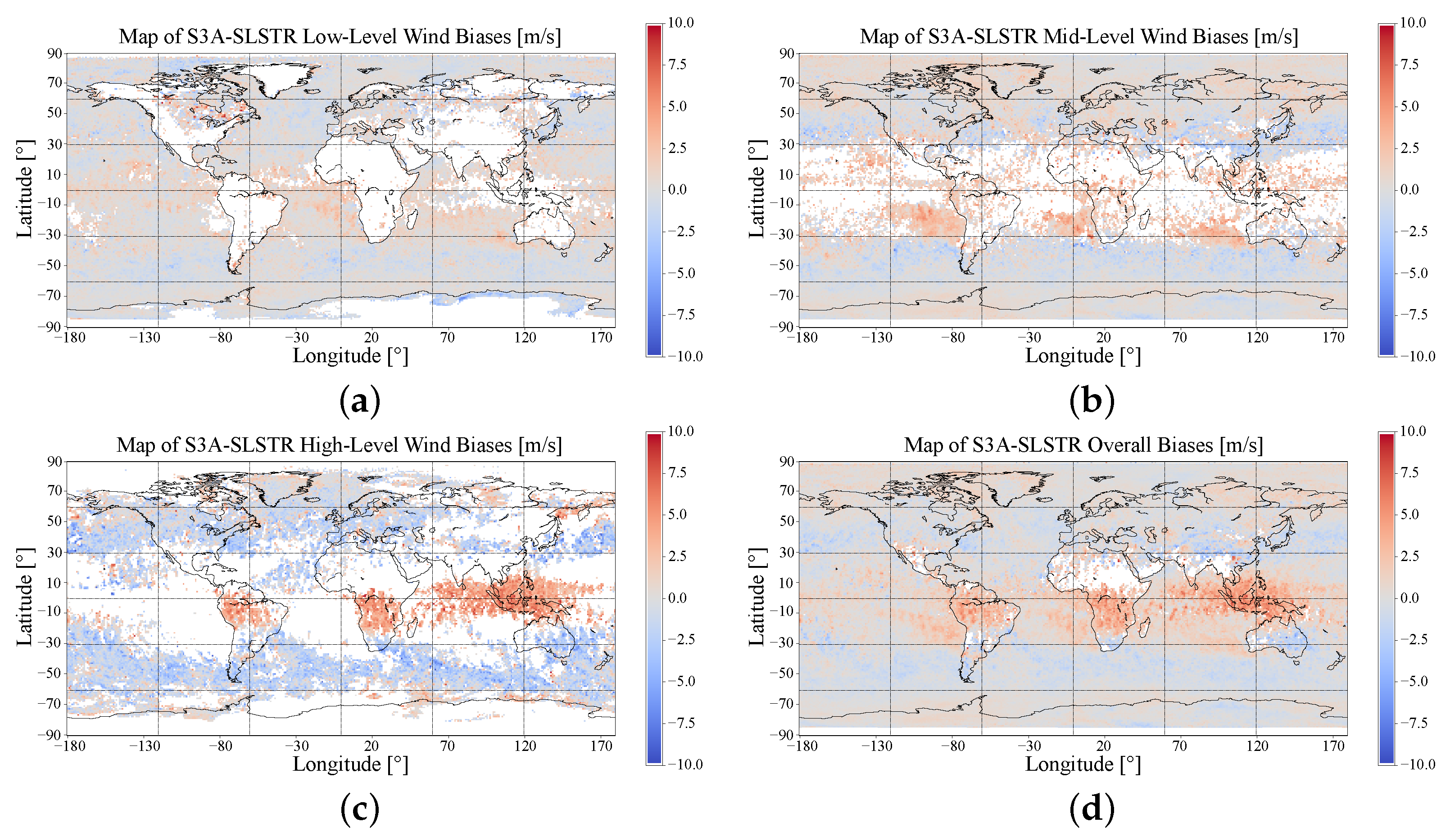
AMVs derived from both satellites present an RMSVD around 5 m/s, which is in line with statistics of AMVs from other sensors exploited by EUMETSAT. The RMS and RMSVD are slightly better for S3B. The higher time gap between the images may explain that behaviour [15]. The motion tracking achieves the same precision, in both cases, but the displacement estimate is divided by a longer time gap, resulting in a lower uncertainty on the wind vector [11]. Overall biases remain low in both cases, although increasing (in absolute value) at high altitudes (<400 hPa). The vast majority of AMVs output by the algorithm are assigned at low and mid altitudes (>600 hPa). Important differences in biases appear at high altitudes between S3A and S3B. This is caused by the difference in coverage of the products: the S3A product is global, it can include many high AMVs in the tropics, where the bias is very high. The S3B product only covers latitudes polewards of 50°, meaning it does not include all these high altitudes AMVs. When limiting the S3A products to AMVs derived polewards of 50° (that is, the areas covered by S3B), AMV biases from S3A and S3B are similar at all altitudes (see Figure 6b,c). The stability of the statistics is also studied time-wise and location-wise. Figure 7 shows the variation of the RMS, RMSVD and bias for both satellites over the period covered by the dataset, and Figure 8 is a world map of the bias AMV—forecast model, for S3A, over the same period.

The statistics remain consistent over time. Regarding spatial stability, the bias varies significantly across the globe, with a noticeable positive bias in the tropical zones. This behaviour is in agreement with observations from other sensors [7]. In some areas (around 10° to 20° latitude in Africa and Asia), too few AMVs of sufficient QI were derived to allow to compute a meaningful bias. It is to be noted that SLSTR is tilted so that it never senses any area South of $-86$° latitude, hence the absence of data at these latitudes in Figure 8.

3.2. Impact of the Projection Grid Resolution

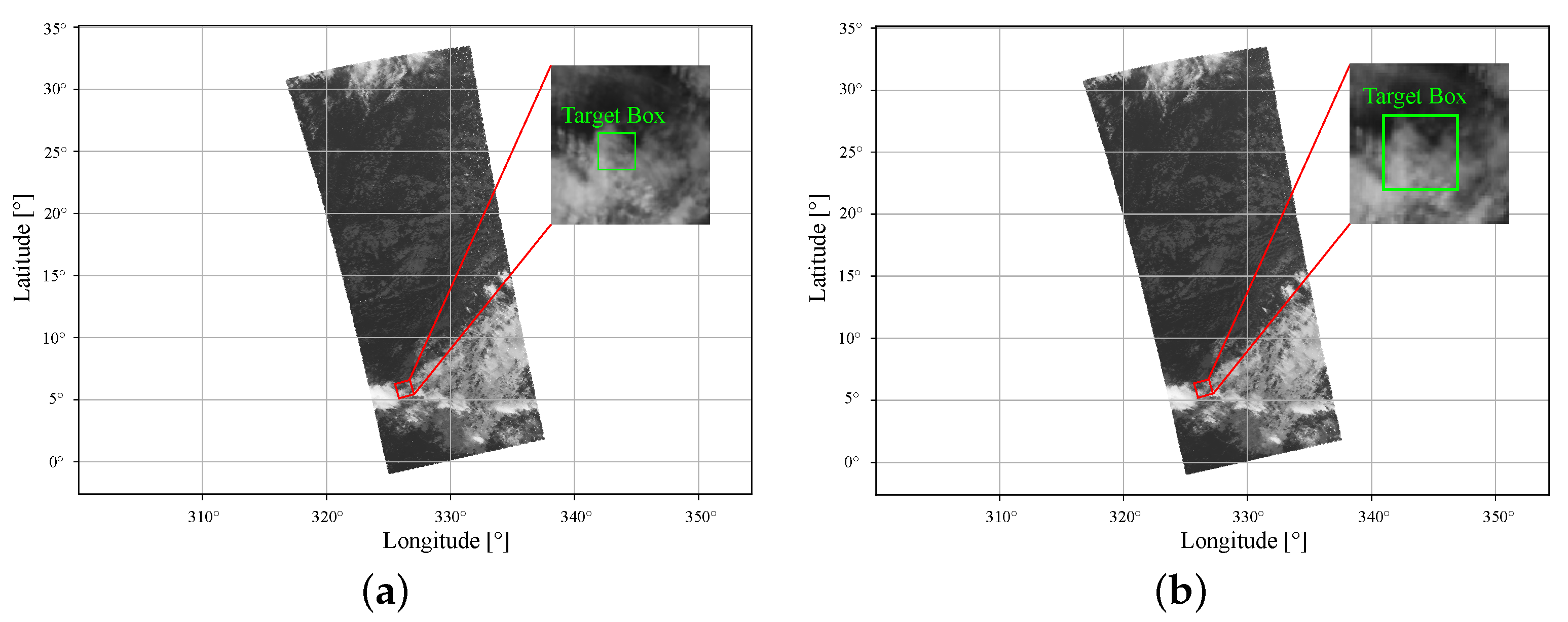
To justify the choice for the projection grid resolution of 1 km, we report hereafter the statistics of AMVs on the same period, but produced with a 2 km projection grid resolution. Projecting with a resolution twice as coarse has two major consequences: the total number of AMVs is divided by four, but the target box covers a geographical area four times as large, as illustrated in Figure 9. The scatter plot of AMVs against the ECMWF forecast model is shown in Figure 10. The corresponding statistics are reported in

Table 2. Comparison of statistics relative to SLSTR AMVs derived during the period of 15 December 2020–15 January 2021, for a projection resolution of 1 km and 2 km.

	S3A, 1 km Projection Resolution, Speed > 2.5 m/s, QI > 60	S3A, 2 km Projection Resolution, Speed > 2.5 m/s, QI > 60
RMS [m/s]	3.60	3.64
RMSVD [m/s]	5.06	5.00
Bias [m/s]	0.08	−0.25
Number of AMVs	9,158,914	1,984,776

. The results, for AMVs of speed $>2.5$ m/s and QI $>60$ are: $RMS=3.64$ m/s, $RMSVD=5.00$ m/s, bias = $-0.25$ m/s and 1,984,776 AMVs were derived. This is about four times less AMVs as for the 1 km resolution, which coincides with the decrease in the number of pixels. The performance statistics remain however similar. Thus, our choice is to keep 1 km as projection resolution to ensure the retrieval of the maximum number of AMVs.

3.3. Comparison between SLSTR and AHVRR Performances

Until the operational release of the SLSTR AMV product, EPS-AVHRR is the only source of AMVs derived from a LEO satellite at EUMETSAT, other sources being MODIS and VIIRS, operated by NOAA. In order to validate SLSTR AMVs, we compare their overall statistics to those of AVHRR AMVs. AVHRR AMVs and SLSTR AMVs are derived from very similar wavelengths, around 10,800 nm, and target and search box sizes are similar. However, there are two major differences between AVHRR and SLSTR AMVs. First, the swath width of SLSTR, 1,420 km, is less than half that of AVHRR, resulting in a much lower number of AMVs derived from each Sentinel-3 satellite. Second, the temporal gap varies a lot depending on which satellite is the reference. In particular, the time gap for S3B products is the highest, with more than a full hour of gap between two successive images. These properties are summarised in

Table 3. Properties of SLSTR and AVHRR, and the associated settings for the derivation of AMVs in dual-satellite mode.

	Sentinel-3A SLSTR	Sentinel-3B SLSTR	Metop-A AVHRR	Metop-B AVHRR	Metop-C AVHRR
Pixel Size at Nadir [m]	1	1	1.1	1.1	1.1
Swath Width [km]	1420	1420	2900	2900	2900
Temporal Gap between images [mins]	39.5	61.5	25	49	27
(as of February 2021)
Target/Search Box Sizes [pixels]	24/100	24/100	28/100	28/100	28/100
Channel Used for AMVs [nm]	10,854	10,854	10,800	10,800	10,800

.

Consequently, far fewer AMVs can be derived daily from either S3A or S3B. To illustrate this, we have computed the overall statistics of AVHRR AMVs for the same period of 15 December 2020 to 15 January 2021. Results are summarised in

Table 4. Statistics relative to SLSTR AMVs and AVHRR derived during the period of 15 December 2020–15 January 2021, for winds faster than 2.5 m/s and QI > 60.

	Sentinel-3A	Sentinel-3B	Metop-A	Metop-B	Metop-C
RMSVD [m/s]	5.06	4.65	4.81	4.35	4.02
Bias [m/s]	0.08	0.29	−0.83	0.13	0.56
Number of AMVs [millions]	9.2	4.7	11.8	16.9	24.4

.

The quality of AMVs is quite comparable across all satellites, in terms of RMSVD and bias. However, the reduced swath width results in significant differences in the number of AMVs. Especially for S3B, the monthly number of AMVs is less than half the equivalent number from any Metop satellite. Furthermore, a higher overlap between reference and dual images implies better performance, since the ground resolution of the pixels is more consistent across images. This fact is reflected in Table 4 by better performance statistics for Metop-C than for Metop-A, which is currently (February 2021, time of writing) drifting away from the nominal orbital plane. Overall, S3A and S3B still represent a monthly contribution of 15 million AMVs with QI > 60. This amount will be a significant source of additional data for NWP systems.

3.4. Comparison to Co-Localised MSG Data

Further validation of the product is made by comparing AMVs to co-located AMVs derived from MSG-SEVIRI. EUMETSAT derives AMVs from bands 2 (visible, at 810 nm), 5 (water vapour, 6,250 nm), 6 (water vapour, 7,350 nm), 9 (thermal infrared, 10,800 nm) and 12 (broadband). In the following, two Meteosat satellites are used for the comparison: Meteosat-11 (MET11), centred at 0°, and Meteosat-8 (MET08), centred at $41.5$° East. Co-location of SLSTR AMVs with AMVs from SEVIRI in the geostationary disks is performed on the period 12 January 2021 to 7 February 2021, with the following criteria:

• The QI of SLSTR vectors shall be above 60, and the QI of SEVIRI vectors shall be above 80.
• There shall be less than 45 min between the two AMVs.
• The distance between AMV locations shall be less than 50 km.
• The difference in height between the two AMVs shall be less than 25 hPa.

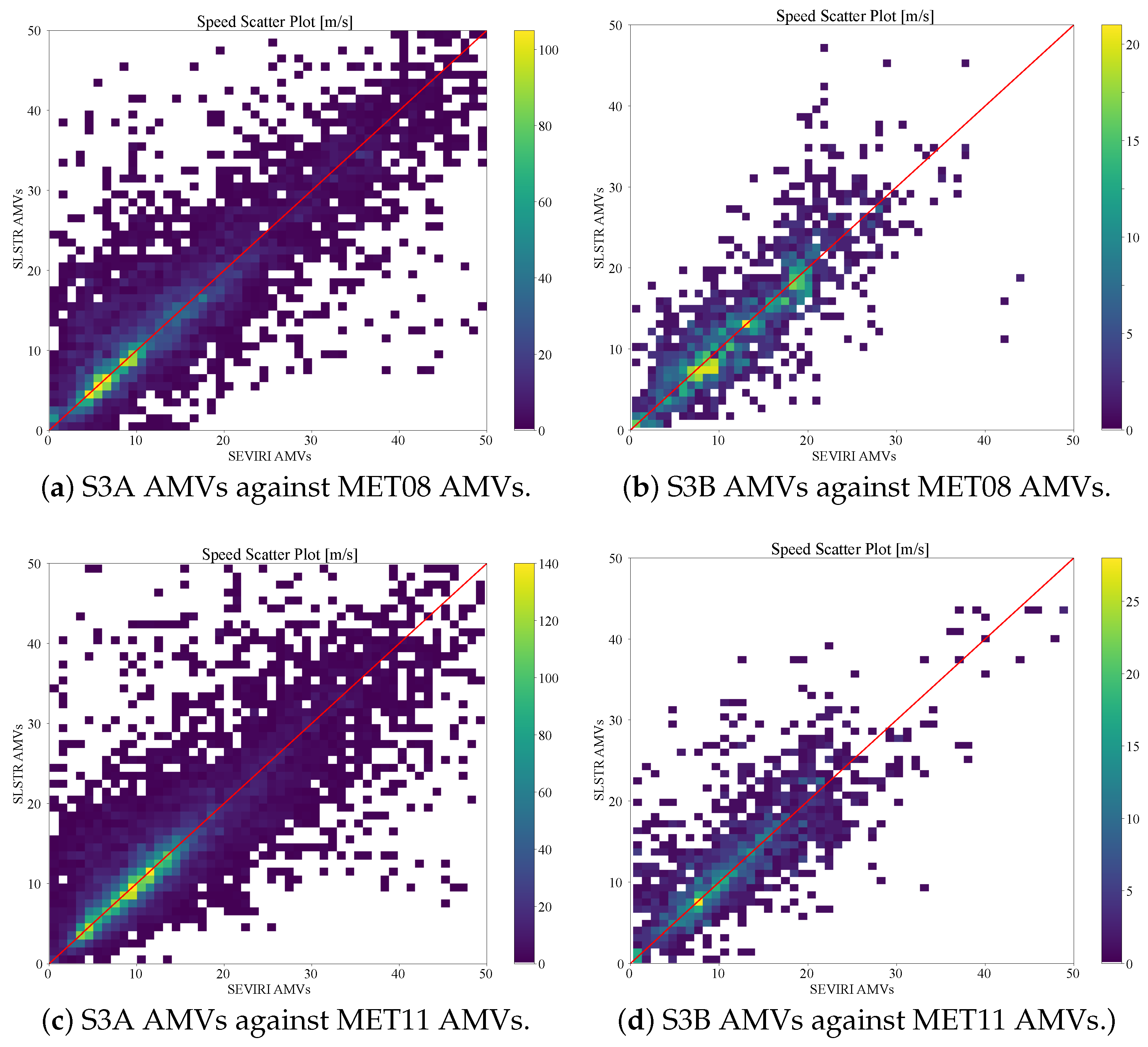
The scatter plots of SEVIRI AMVs, for MET08 and MET11, against SLSTR AMVs, for S3A and S3B, are shown in Figure 11.

The statistics are reported in

Table 5. Statistics on the comparison between matched AMVs from SLSTR and SEVIRI, for the period 5 January 2021–31 January 2021, for vectors of QI > 60.

	S3A/MET08	S3B/MET08	S3A/MET11	S3B/MET11
RMS [m/s]	6.90	4.32	6.50	5.16
RMSVD [m/s]	8.47	5.90	8.33	7.13
Bias, SLSTR—SEVIRI [m/s]	0.83	0.36	0.40	0.83
Number of AMVs matched	7339	1835	9482	1632

.

Given that S3B AMVs cover latitudes above 50°, there is minimal overlap between the S3B products coverage and the coverage of geo-winds products, resulting in a meagre number of matches for S3B. Nevertheless, in all cases, there is good agreement between the two sets of AMVs, with a noticeable positive bias. Considering that the biases against the model are high in the tropical regions (see Figure 8) which are the most represented regions in the geostationary disks, this is not surprising. Apart from the bias, the RMSVD suggests there is consistency between geostationary and LEO AMVs.

4. Conclusions

EUMETSAT presently derives offline and routinely AMVs from pairs of images from Sentinel-3A and B. When checked against the ECMWF forecast model, the quality of AMVs is similar to that of AMVs derived from AVHRR data. This will guarantee consistency between operational AMV products disseminated by EUMETSAT. The narrower swath of SLSTR, compared to AVHRR, results in lower coverage, and then, far fewer AMVs are derived daily from SLSTR than from AVHRR. However, using an equal-area projection grid allows the mitigation of some caveats of the current coregistration method used for AVHRR. SLSTR AMV products, like AVHRR AMV products, will help to measure winds at high latitudes (polewards of 50°), not covered by sensors on board geostationary satellites. After validation of the offline products by end users, EUMETSAT plans to start disseminating SLSTR AMV products operationally in 2022.

References

1. English, S.; McNally, T.; Bormann, N.; Salonen, K.; Matricardi, M.; Moranyi, A.; Rennie, M.; Janisková, M.; Di Michele, S.; Geer, A.; et al. Impact of satellite data. In ECMWF Tech. Memo No 711; European Centre for Medium-Range Weather Forecasts: Reading, UK, 2013. [Google Scholar]
2. Le Marshall, J.; Mills, G.; Pescod, N.; Seecamp, R.; Puri, K.K.; Stewart, P.; Leslie, L.M.; Rea, A. The estimation of high density atmospheric motion vectors and their application to operational numerical weather prediction. Aust. Meteorol. Mag. 2002, 51, 173–180. [Google Scholar]
3. Kim, M.; Kim, H.M.; Kim, J.W.; Kim, S.M.; Velden, C.; Hoover, B. Effect of enhanced satellite-derived atmospheric motion vectors on numerical weather prediction in East Asia using an adjoint-based observation impact method. Weather Forecast. 2017, 32, 579–594. [Google Scholar] [CrossRef]
4. Key, J.R.; Santek, D.; Velden, C.S.; Bormann, N.; Thepaut, J.N.; Riishojgaard, L.P. Cloud-drift and water vapor winds in the polar regions from MODIS. IEEE Trans. Geosci. Remote Sens. 2013, 41, 482–492. [Google Scholar] [CrossRef] [Green Version]
5. Lazzara, M.A.; Dworak, R.; Santek, D.A.; Hoover, B.T.; Velden, C.S.; Key, J.R. High-latitude atmospheric motion vectors from composite satellite data. J. Appl. Meteorol. Climatol. 2014, 53, 534–547. [Google Scholar] [CrossRef]
6. Borde, R.; Carranza, M.; Hautecoeur, O.; Barbieux, K. Winds of Change for Future Operational AMV at EUMETSAT. Multidiscip. Digit. Publ. Inst. 2019, 11, 2111. [Google Scholar] [CrossRef] [Green Version]
7. Borde, R.; Hautecoeur, O.; Carranza, M. EUMETSAT global AVHRR wind product. J. Atmos. Ocean. Technol. 2016, 33, 429–438. [Google Scholar] [CrossRef]
8. Bartolomei, D.M. Generic Projection Tool—Technical Note. In EUMETSAT Internal Document; EUM/RSP/TEN/18/1030434; EUMETSAT: Darmstadt, Germany, 2019. [Google Scholar]
9. Mills, S. The ground track oblique Cassini projection used for producing VIIRS mapped imagery. In Proceedings of the Earth Observing Systems XIX. International Society for Optics and Photonics, San Diego, DC, USA, 18–20 August 2014; Volume 9218. [Google Scholar]
10. Borde, R.; García-Pereda, J. Impact of wind guess on the tracking of atmospheric motion vectors. J. Atmos. Ocean. Technol. 2014, 31, 458–467. [Google Scholar] [CrossRef] [Green Version]
11. Hautecoeur, O.; Borde, R. Derivation of wind vectors from AVHRR/Metop at EUMETSAT. J. Atmos. Ocean. Technol. 2017, 34, 1645–1659. [Google Scholar] [CrossRef]
12. Borde, R.; Doutriaux-Boucher, M.; Dew, G.; Carranza, M. A direct link between feature tracking and height assignment of operational EUMETSAT atmospheric motion vectors. J. Atmos. Ocean. Technol. 2014, 31, 33–46. [Google Scholar] [CrossRef]
13. Karhila, V.; Hernandez-Carrascal, A. BUFR: A meteorological code for the 21st century. In Proceedings of the EUMETSAT Meteorological Satellite Conference, Córdoba, Spain, 20–24 September 2010; Volume 5. [Google Scholar]
14. Holmlund, K. The utilization of statistical properties of satellite-derived atmospheric motion vectors to derive quality indicators. Weather Forecast. 1998, 13, 1093–1104. [Google Scholar]
15. García-Pereda, J.; Borde, R. The impact of the tracer size and the temporal gap between images in the extraction of atmospheric motion vectors. J. Atmos. Ocean. Technol. 2014, 31, 1761–1770. [Google Scholar] [CrossRef] [Green Version]
Figure 1. Successive traces of scans from (a) Sentinel-3A (red), with the overlap in darker red, and (be) Sentinel-3A (red) and Sentinel-3B (blue), showing the overlap in which AMVs can be derived (purple).
Remotesensing 13 01702 g001
Figure 2. Principle of the co-registration of images for the derivation of AMVs from EPS-AVHRR: (a) values from the dual image are mapped, by latitude/longitude, to the frame of the reference image; (b) the values are then assigned to pixels of the reference grid following a nearest neighbour criterion; (c) then, the values are interpolated to the whole reference frame by bilinear interpolation.
Remotesensing 13 01702 g002
Figure 3. Principle of the co-registration of images for the derivation of AMVs from S3-SLSTR: (a) values of both PDUs are projected onto an equal-area grid; (b) the values are then assigned to pixels of the grid following a nearest neighbour criterion; (c) then, the values are interpolated to the whole reference frame by bilinear interpolation.
Remotesensing 13 01702 g003
Figure 4. Steps of the motion tracking method.
Remotesensing 13 01702 g004
Figure 5. Scatter plot of wind speeds, ECMWF forecast model against AMVs, for the period of 15 December 2020–15 January 2021, for (a) S3A, (b) S3B and (c) S3A polewards of 50°, for winds faster than 2.5 m/s and for QI > 60.
Remotesensing 13 01702 g005
Figure 6. Speed biases, RMS, RMSVD and number of SLSTR AMVs as functions of the altitude, for the period of 15 December 2020–15 January 2021, for (a) S3A and (b) S3B, for winds faster than 2.5 m/s and for QI > 60. (c) is a similar plot for S3A, but limited to AMVs polewards of 50°, so that AMV statistics of S3A and S3B can be compared. A positive bias means that AMVs are faster than their equivalent forecast winds; conversely a negative bias means AMVs are slower.
Remotesensing 13 01702 g006
Figure 7. Evolution of daily statistics of SLSTR AMVs, for winds faster than 2.5 m/s and for QI > 60.
Remotesensing 13 01702 g007
Figure 8. Speed bias AMV—forecast, per latitude/longitude cell, for S3A over the period 15 December 2020–15 January 2021, for winds faster than 2.5 m/s and QI > 60, for (a) low-level winds (pressure between 1000 and 700 hPa), (b) mid-level winds (pressure between 700 and 400 hPa), (c) high-level winds (pressure between 400 and 100 hPa) and (d) all winds.
Remotesensing 13 01702 g008
Figure 9. SLSTR scans from S3B, on 14 January 2021, from 00:08:51 to 00:17:51 UTC, projected on a grid of (a) 1 km of resolution and (b) 2 km of resolution. A zoom of the same geographical area (in red) and a target box of 24 × 24 pixels are shown in both cases, revealing the difference in size of features tracked between the two cases.
Remotesensing 13 01702 g009
Figure 10. Scatter plot of wind speeds, ECMWF forecast model against AMVs, for the period of 15 December 2020–15 January 2021, for S3A, with AMVs derived from 2 km grids.
Remotesensing 13 01702 g010
Figure 11. Scatter plot of wind speeds, SLSTR AMVs against SEVIRI AMVs, for the period 12 January 2021–7 February 2021.
Remotesensing 13 01702 g011