
Modeling the Spatial Dynamics of Soil Organic Carbon Using Remotely-Sensed Predictors in Fuzhou City, China

 , ,
, ,  ,
, 
 and
and
Abstract
1. Introduction
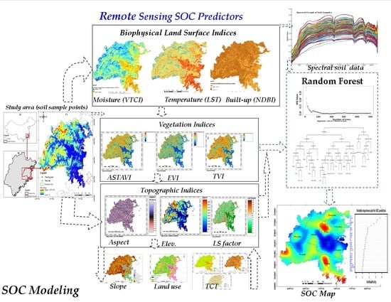
2. Materials and Methods
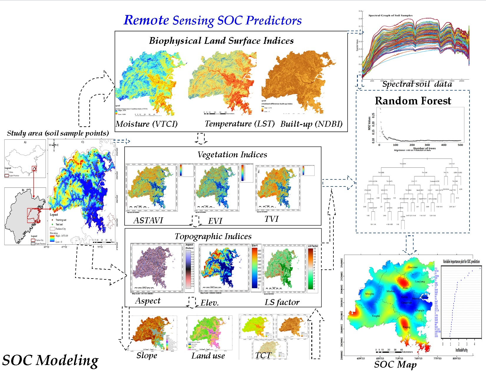
2.1. Description of the Study Area and Sampling Locations
2.2. Soil Sampling and Laboratory Analysis
2.3. Description and Preprocessing of Landsat-8 Images, and Soil Spectral Data Transformations
2.4. Data Sources, Software, and Extraction of Environmental Covariates
2.5. Statistical Analysis, Spatial Modeling, and Validation
3. Results
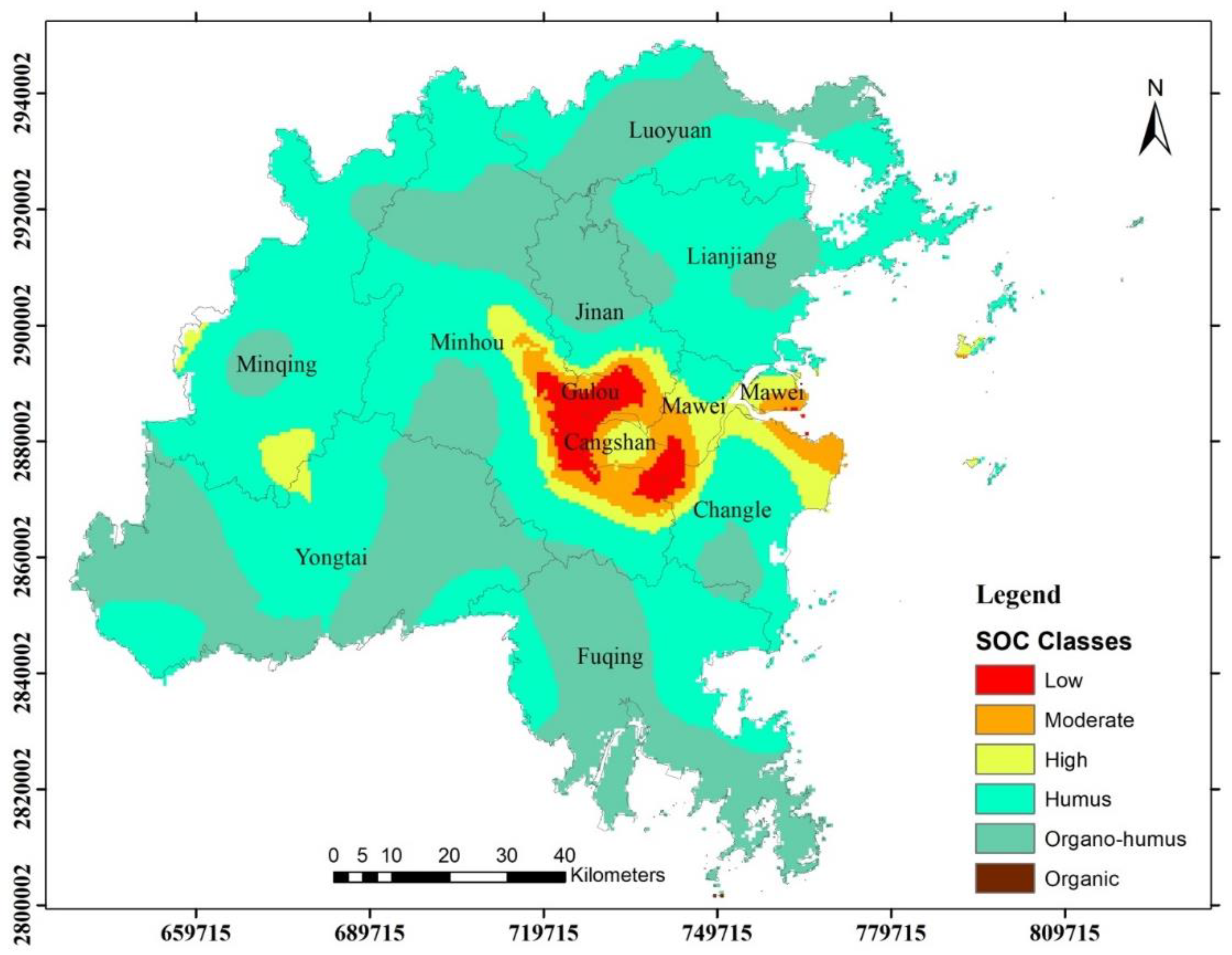
3.1. Spatial Prediction of SOC and Model Validation
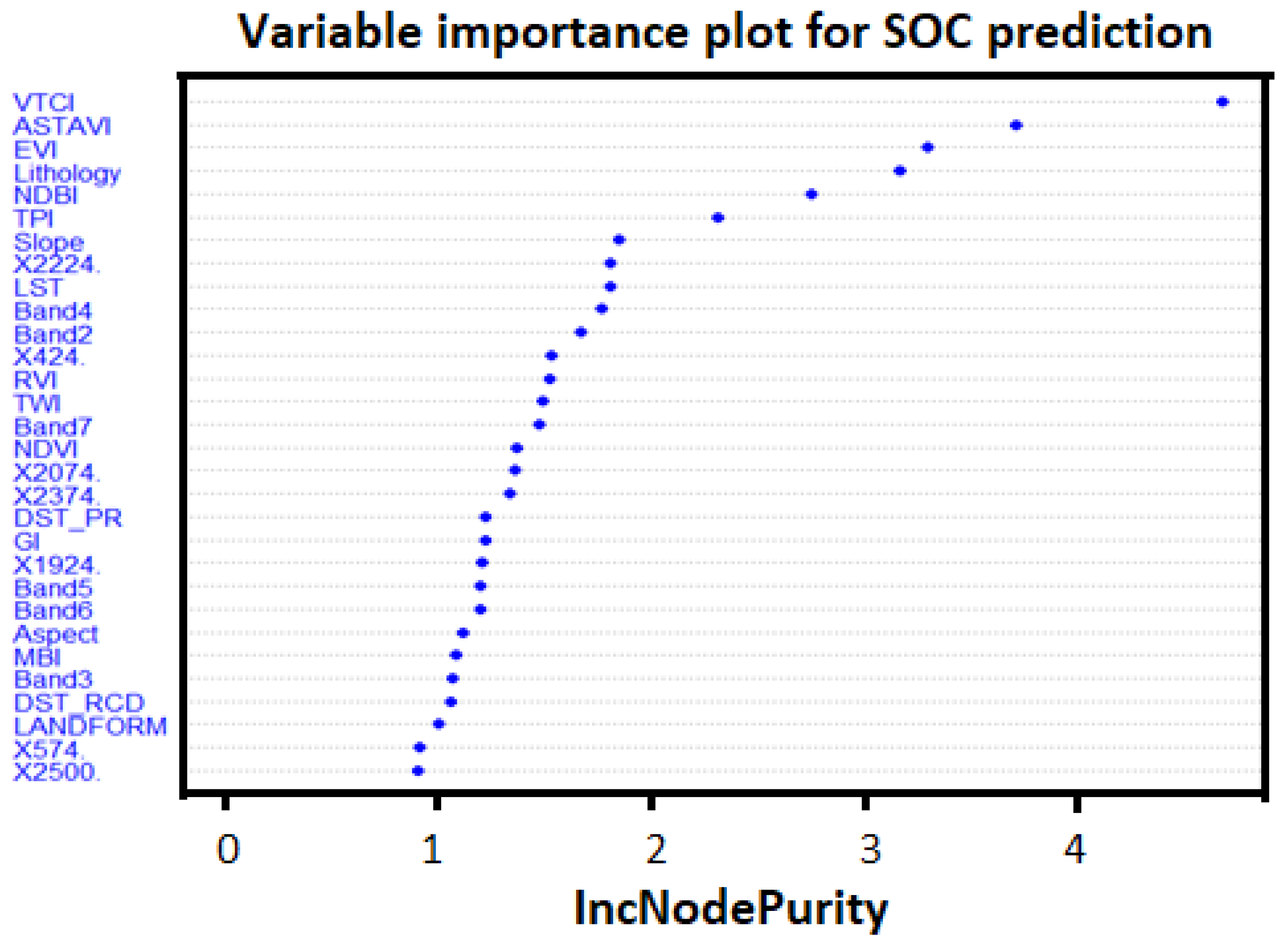
3.2. Importance of Environmental Variables
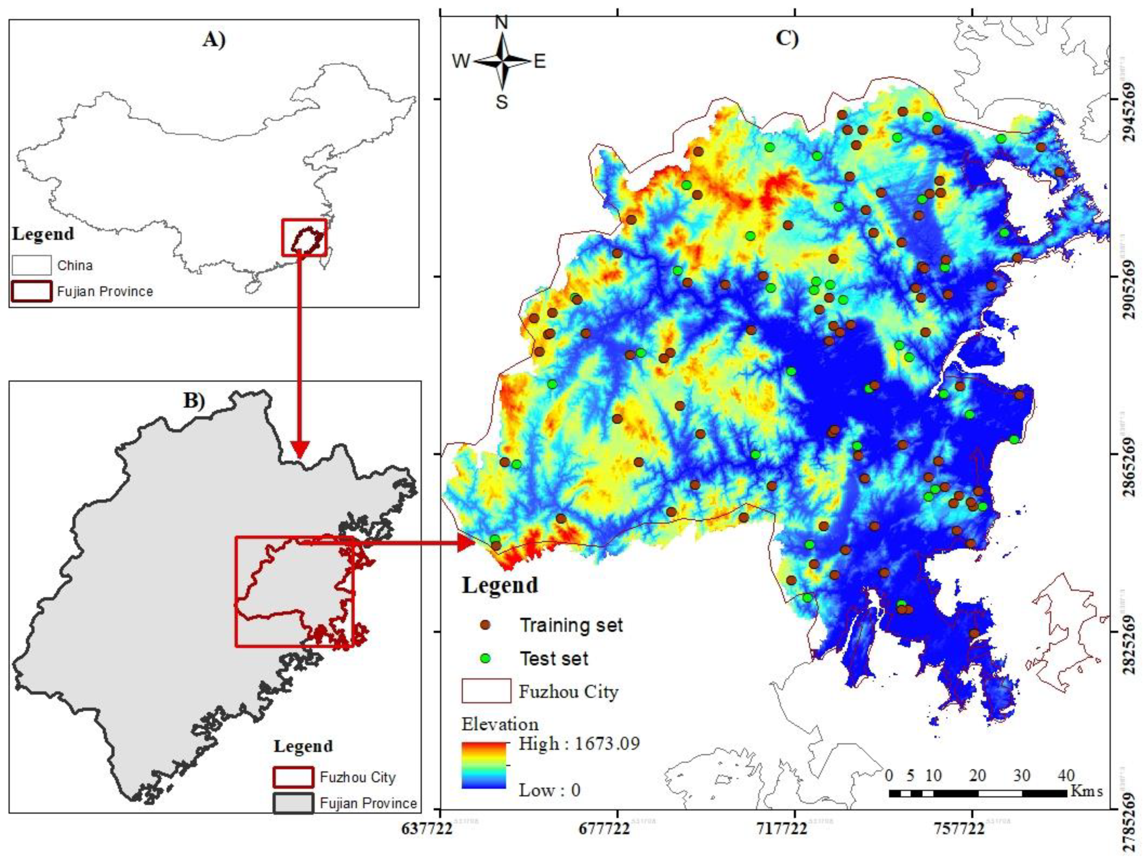
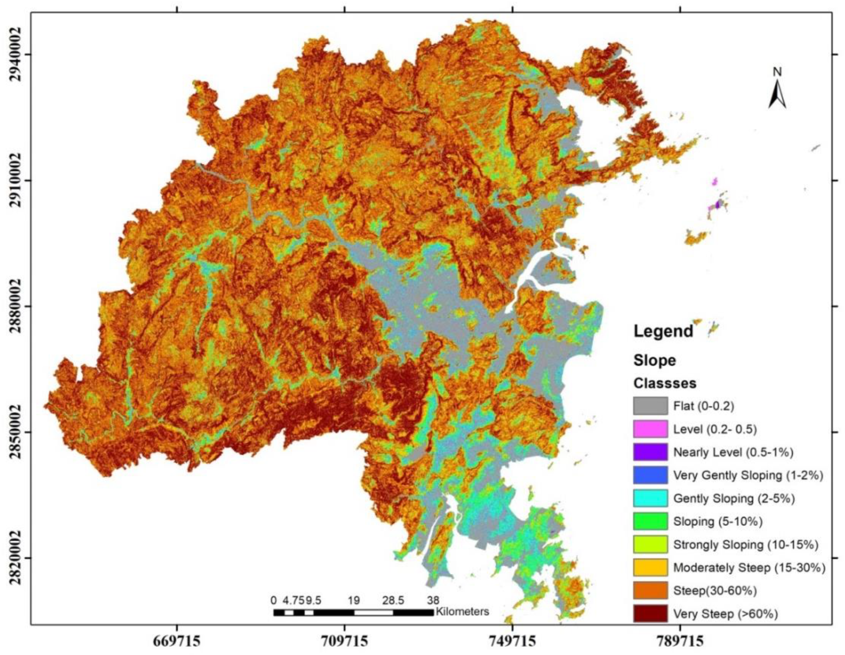
3.3. Influence of Topographic and Vegetation Indices
3.4. SOC Distribution across Landform, Land Use, and Lithology
4. Discussion
4.1. Spatial Variability of SOC
4.2. Importance of Environmental Variables
4.3. Influence of Topographic and Vegetation Indices
4.4. SOC Distribution across the Landform, Land Use, and Lithology
5. Conclusions
Author Contributions
Funding
Institutional Review Board Statement
Informed Consent Statement
Data Availability Statement
Acknowledgments
Conflicts of Interest
References
- Tiessen, H.; Cuevas, E.; Chacon, P. The role of soil organic matter in sustaining soil fertility. Nature 1994, 371, 783–785. [Google Scholar] [CrossRef]
- Oyonarte, C.; Aranda, V.; Durante, P. Soil surface properties in Mediterranean mountain ecosystems: Effects of environmental factors and implications of management. For. Ecol. Manag. 2008, 254, 156–165. [Google Scholar] [CrossRef]
- Yan, Y.; Kuang, W.; Zhang, C.; Chen, C. Impacts of impervious surface expansion on soil organic carbon—A spatially explicit study. Sci. Rep. 2015, 5, 17905. [Google Scholar] [CrossRef] [PubMed]
- Pouyat, R.; Groffman, P.; Yesilonis, I.; Hernandez, L. Soil carbon pools and fluxes in urban ecosystems. Environ. Pollut. 2002, 116, S107–S118. [Google Scholar] [CrossRef]
- Chen, W.Y. The role of urban green infrastructure in offsetting carbon emissions in 35 major Chinese cities: A nationwide estimate. Cities 2015, 44, 112–120. [Google Scholar] [CrossRef]
- Wang, S.; Zhuang, Q.; Jia, S.; Jin, X.; Wang, Q. Spatial variations of soil organic carbon stocks in a coastal hilly area of China. Geoderma 2017, 314, 8–19. [Google Scholar] [CrossRef]
- Raciti, S.M.; Hutyra, L.R.; Rao, P.; Finzi, A.C. Inconsistent definitions of “urban” result in different conclusions about the size of urban carbon and nitrogen stocks. Ecol. Appl. 2012, 22, 1015–1035. [Google Scholar] [CrossRef]
- Xia, X.; Yang, Z.; Xue, Y.; Shao, X.; Yu, T.; Hou, Q. Spatial analysis of land use change effect on soil organic carbon stocks in the eastern regions of China between 1980 and 2000. Geosci. Front. 2017, 8, 597–603. [Google Scholar] [CrossRef]
- McBratney, A.; Mendonça Santos, M.; Minasny, B. On digital soil mapping. Geoderma 2003, 117, 3–52. [Google Scholar] [CrossRef]
- Curtin, D.; Beare, M.H.; Hernandez-Ramirez, G. Temperature and Moisture Effects on Microbial Biomass and Soil Organic Matter Mineralization. Soil Sci. Soc. Am. J. 2012, 76, 2055–2067. [Google Scholar] [CrossRef]
- Wang, D.; He, N.; Wang, Q.; Lü, Y.; Wang, Q.; Xu, Z.; Zhu, J. Effects of Temperature and Moisture on Soil Organic Matter Decomposition Along Elevation Gradients on the Changbai Mountains, Northeast China. Pedosphere 2016, 26, 399–407. [Google Scholar] [CrossRef]
- Schrumpf, M.; Kaiser, K.; Schulze, E.-D. Soil Organic Carbon and Total Nitrogen Gains in an Old Growth Deciduous Forest in Germany. PLoS ONE 2014, 9, e89364. [Google Scholar] [CrossRef]
- Bartalis, Z.; Wagner, W.; Naeimi, V.; Hasenauer, S.; Scipal, K.; Bonekamp, H.; Figa, J.; Anderson, C. Initial soil moisture retrievals from the METOP-A Advanced Scatterometer (ASCAT). Geophys. Res. Lett. 2007, 34. [Google Scholar] [CrossRef]
- Zhang, D.; Tang, R.; Zhao, W.; Tang, B.; Wu, H.; Shao, K.; Li, Z.L. Surface soil water content estimation from thermal remote sensing based on the temporal variation of land surface temperature. Remote Sens. 2014, 6, 3170–3187. [Google Scholar] [CrossRef]
- Zhuo, L.; Tao, H.; Wei, H.; Chengzhen, W. Plantation in Fujian Province, China. PLoS ONE 2016, 11, 151527. [Google Scholar]
- Liu, Y.; Su, C.; Zhang, H.; Li, X.; Pei, J. Interaction of Soil Heavy Metal Pollution with Industrialisation and the Landscape Pattern in Taiyuan City, China. PLoS ONE 2014, 9, e105798. [Google Scholar]
- Roy, D.P.; Wulder, M.A.; Loveland, T.R.; Woodcock, C.E.; Allen, R.G.; Anderson, M.C.; Helder, D.; Irons, J.R.; Johnson, D.M.; Kennedy, R.; et al. Landsat-8: Science and product vision for terrestrial global change research. Remote Sens. Environ. 2014, 145, 154–172. [Google Scholar] [CrossRef]
- U.S. Department of Interior. Using the USGS Landsat 8 Product. 2013. Available online: http://landsat.usgs.gov (accessed on 27 April 2021).
- Savitzky, A.; Golay, M.J. Smoothing and Differentiation of Data by Simplified Least Squares Procedures. Anal. Chem. 1951, 40, 1627–1639. [Google Scholar] [CrossRef]
- Wei, Z.-Q.; Wu, S.-H.; Zhou, S.-L.; Li, J.-T.; Zhao, Q.-G. Soil Organic Carbon Transformation and Related Properties in Urban Soil Under Impervious Surfaces. Pedosphere 2014, 24, 56–64. [Google Scholar] [CrossRef]
- Jenness, J. Topographic Position Index (tpi_jen.avx_extension) for Arcview 3.x, v.1.3a, Jenness Enterprises [EB/OL]. 2006. Available online: http://www.jennessent.com/arcview/tpi.htm (accessed on 12 June 2018).
- Rasul, A.; Balzter, H.; Smith, C. Spatial variation of the daytime Surface Urban Cool Island during the dry season in Erbil, Iraqi Kurdistan, from Landsat 8. Urban Clim. 2015, 14, 176–186. [Google Scholar] [CrossRef]
- Thompson, J.A.; Bell, J.C.; Butler, C.A. Digital elevation model resolution: Effects on terrain attribute calculation and quantitative soil-landscape modeling. Geoderma 2001, 100, 67–89. [Google Scholar] [CrossRef]
- Wan, Z.; Wang, P.; Li, X. Using MODIS Land Surface Temperature and Normalized Difference Vegetation Index products for monitoring drought in the southern Great Plains, USA. Int. J. Remote Sens. 2004, 25, 61–72. [Google Scholar] [CrossRef]
- Avdan, U.; Jovanovska, G. Algorithm for Automated Mapping of Land Surface Temperature Using LANDSAT 8 Satellite Data. J. Sens. 2016, 2016, 1480307. [Google Scholar] [CrossRef]
- Rondeaux, G.; Steven, M.; Baret, F. Optimization of soil-adjusted vegetation indices. Remote Sens. Environ. 1996, 55, 95–107. [Google Scholar] [CrossRef]
- Ford, W.M.; Menzel, M.A.; Odom, R.H. Elevation, aspect, and cove size effects on southern Appalachian salamanders. Southeast. Nat. 2002, 1, 315–324. [Google Scholar] [CrossRef]
- Weier, J.; Herring, D. Measuring Vegetation (NDVI and EVI). NASA Earth Observatory. 2000. Available online: http://earthobservatory.nasa.gov/Features/MeasuringVegetation/ (accessed on 27 April 2021).
- Chejarla, V.R.; Maheshuni, P.K.; Mandla, V.R. Quantification of LST and CO2 levels using Landsat-8 thermal bands on urban environment. Geocarto Int. 2016, 31, 913–926. [Google Scholar] [CrossRef]
- Pennock, D.J.; Zebarth, B.J.; De Jong, E. Landform classification and soil distribution in hummocky terrain, Saskatchewan, Canada. Geoderma 1987, 40, 297–315. [Google Scholar] [CrossRef]
- Sørensen, R. Topographical Influence on Soil Chemistry; Sveriges lantbruksuniv: Uppsala, Sweden, 2006. [Google Scholar]
- Taghizadeh-Mehrjardi, R.; Nabiollahi, K.; Kerry, R. Digital mapping of soil organic carbon at multiple depths using different data mining techniques in Baneh region, Iran. Geoderma 2016, 266, 98–110. [Google Scholar] [CrossRef]
- Möller, M.; Volk, M. Effective map scales for soil transport processes and related process domains—Statistical and spatial characterization of their scale-specific inaccuracies. Geoderma 2015, 247, 151–160. [Google Scholar] [CrossRef]
- Li, X.; McCarty, G.W.; Karlen, D.L.; Cambardella, C.A. Topographic metric predictions of soil redistribution and organic carbon in Iowa cropland fields. Catena 2018, 160, 222–232. [Google Scholar] [CrossRef]
- Chuai, X.-W.; Huang, X.-J.; Wang, W.-J.; Zhang, M.; Lai, L.; Liao, Q.-L. Spatial Variability of Soil Organic Carbon and Related Factors in Jiangsu Province, China. Pedosphere 2012, 22, 404–414. [Google Scholar] [CrossRef]
- Mróz, M.; Sobieraj, A. Comparison of Several Vegetation Indices Calculated on the Basis of a Seasonal Spot XS Time Series, and Their Suitability for Land Cover and Agricultural Crop Identification. Tech. Sci. 2004, 7, 39–66. [Google Scholar]
- Van Khoa, P.; Hoa, N.H.; Tuan, D.A. Using remote sensing indices to reduce effects of hillshade on LANDSAT 8 imagery. Available online: https://vnuf.edu.vn/documents/454250/1808434/9.pdf (accessed on 27 April 2021).
- Payero, J.O.; Neale, C.M.U.; Wright, J.L. Comparison of eleven vegetation indices for estimating plant height of alfalfa and grass. Appl. Eng. Agric. 2004, 20, 385–393. [Google Scholar] [CrossRef]
- Patel, N.R.; Parida, B.R.; Venus, V.; Saha, S.K.; Dadhwal, V.K. Analysis of agricultural drought using vegetation temperature condition index (VTCI) from Terra/MODIS satellite data. Environ. Monit. Assess. 2012, 184, 7153–7163. [Google Scholar] [CrossRef]
- Ahmad, F. Spectral vegetation indices performance evaluated for Cholistan Desert. J. Geogr. Reg. Plan. 2012, 5, 165–172. [Google Scholar]
- Mróz, M.; Sciences, A.S.-T. Undefined Comparison of several vegetation indices calculated on the basis of a seasonal SPOT XS time series, and their suitability for land cover and agricultural crop identification. Tech. Sci. 2004, 7, 39–66. [Google Scholar]
- Kandwal, R.; Jeganathan, C.; Tolpekin, V.; Kushwaha, S.P.S. Discriminating the invasive species, ‘Lantana’ using vegetation indices. J. Indian Soc. Remote Sens. 2009, 37, 275–290. [Google Scholar] [CrossRef]
- Peuquet, D.J. An algorithm for calculating minimum Euclidean distance between two geographic features. Comput. Geosci. 1992, 18, 989–1001. [Google Scholar] [CrossRef]
- Barsi, J.; Lee, K.; Kvaran, G.; Markham, B.; Pedelty, J. The Spectral Response of the Landsat-8 Operational Land Imager. Remote Sens. 2014, 6, 10232–10251. [Google Scholar] [CrossRef]
- Erbek, F.S.; Özkan, C.; Taberner, M. Comparison of maximum likelihood classification method with supervised artificial neural network algorithms for land use activities. Int. J. Remote Sens. 2004, 25, 1733–1748. [Google Scholar] [CrossRef]
- FAO. Guidelines for Soil Description, 4th ed.; Food and Agriculture Organization of the United Nations: Rome, Italy, 2006; ISBN 92-5-105521-1. [Google Scholar]
- Grover, A.; Singh, R. Monitoring Spatial Patterns of Land Surface Temperature and Urban Heat Island for Sustainable Megacity. Environ. Urban. ASIA 2016, 7, 38–54. [Google Scholar] [CrossRef]
- Hengl, T.; Heuvelink, G.B.M.; Kempen, B.; Leenaars, J.G.B.; Walsh, M.G.; Shepherd, K.D.; Sila, A.; MacMillan, R.A.; De Jesus, J.M.; Tamene, L.; et al. Mapping soil properties of Africa at 250 m resolution: Random forests significantly improve current predictions. PLoS ONE 2015, 10, e0125814. [Google Scholar] [CrossRef] [PubMed]
- Nielsen, D.R.; Bouma, J. Soil spatial variability. In Proceedings of the Workshop of the ISSS (Int. Society of Soil Science) and the SSSA (Soil Science Society of America), Las Vegas, NV, USA, 30 November–1 December 1985. [Google Scholar]
- Grimm, R.; Behrens, T.; Märker, M.; Elsenbeer, H. Soil organic carbon concentrations and stocks on Barro Colorado Island—Digital soil mapping using Random Forests analysis. Geoderma 2008, 146, 102–113. [Google Scholar] [CrossRef]
- Breiman, L. Classification and regression trees. In Encyclopedia of Ecology; CRC Press: Boca Raton, FL, USA, 1984. [Google Scholar]
- Wiesmeier, M.; Barthold, F.; Blank, B.; Kögel-Knabner, I. Digital mapping of soil organic matter stocks using Random Forest modeling in a semi-arid steppe ecosystem. Plant Soil 2011, 340, 7–24. [Google Scholar] [CrossRef]
- Sorenson, P.T.; Small, C.; Tappert, M.C.; Quideau, S.A.; Drozdowski, B.; Underwood, A.; Janz, A. Monitoring organic carbon, total nitrogen, and pH for reclaimed soils using field reflectance spectroscopy. Can. J. Soil Sci. 2017, 97, 241–248. [Google Scholar] [CrossRef]
- Liaw, A.; Wiener, M. Classification and Regression by randomForest. R News 2002, 2, 18–22. [Google Scholar]
- Forkuor, G.; Hounkpatin, O.K.L.; Welp, G.; Thiel, M. High resolution mapping of soil properties using Remote Sensing variables in south-western Burkina Faso: A comparison of machine learning and multiple linear regression models. PLoS ONE 2017, 12, e0170478. [Google Scholar] [CrossRef]
- Probst, P.; Boulesteix, A.L. To tune or not to tune the number of trees in random forest. J. Mach. Learn. Res. 2018, 18, 6673–6690. [Google Scholar]
- Ridgeway, G. gbm: Generalized Boosted Regression Models. R Packag. Version 2006, 1, 55. [Google Scholar]
- Minasny, B.; McBratney, A.B.; Malone, B.P.; Wheeler, I. Chapter One—Digital Mapping of Soil Carbon. Adv. Agron. 2013, 118, 1–47. [Google Scholar]
- Zhang, L.; Liu, Y.; Li, X.; Huang, L.; Yu, D.; Shi, X.; Chen, H.; Xing, S. Effects of soil map scales on simulating soil organic carbon changes of upland soils in Eastern China. Geoderma 2018, 312, 159–169. [Google Scholar] [CrossRef]
- Nawar, S.; Mouazen, A. Comparison between Random Forests, Artificial Neural Networks and Gradient Boosted Machines Methods of On-Line Vis-NIR Spectroscopy Measurements of Soil Total Nitrogen and Total Carbon. Sensors 2017, 17, 2428. [Google Scholar] [CrossRef] [PubMed]
- Alvarez, R.; Lavado, R.S. Climate, organic matter and clay content relationships in the Pampa and Chaco soils, Argentina. Geoderma 1998, 83, 127–141. [Google Scholar] [CrossRef]
- Jenny, H.; Amundson, R. Factors of Soil Formation: A System of Quantitative Pedology; Courier Corporation: North Chelmsford, MA, USA, 1994. [Google Scholar]
- Sun, W.; Li, X.; Niu, B. Prediction of soil organic carbon in a coal mining area by Vis-NIR spectroscopy. PLoS ONE 2018, 13, e0196198. [Google Scholar] [CrossRef] [PubMed]
- Purevdorj, T.S.; Tateishi, R.; Ishiyama, T.; Honda, Y. Relationships between percent vegetation cover and vegetation indices. Int. J. Remote Sens. 1998, 19, 3519–3535. [Google Scholar] [CrossRef]
- Peng, Y.; Xiong, X.; Adhikari, K.; Knadel, M.; Grunwald, S.; Greve, M.H. Modeling Soil Organic Carbon at Regional Scale by Combining Multi-Spectral Images with Laboratory Spectra. PLoS ONE 2015, 10, e0142295. [Google Scholar] [CrossRef]
- Raciti, S.M.; Groffman, P.M.; Jenkins, J.C.; Pouyat, R.V.; Fahey, T.J.; Pickett, S.T.A.; Cadenasso, M.L. Accumulation of Carbon and Nitrogen in Residential Soils with Different Land-Use Histories. Ecosystems 2011, 14, 287–297. [Google Scholar] [CrossRef]
- Gray, J.M.; Bishop, T.F.A.; Wilson, B.R. Factors Controlling Soil Organic Carbon Stocks with Depth in Eastern Australia. Soil Sci. Soc. Am. J. 2015, 79, 1741. [Google Scholar] [CrossRef]
- Vohland, M.; Ludwig, M.; Thiele-Bruhn, S.; Ludwig, B.; Vohland, M.; Ludwig, M.; Thiele-Bruhn, S.; Ludwig, B. Quantification of Soil Properties with Hyperspectral Data: Selecting Spectral Variables with Different Methods to Improve Accuracies and Analyze Prediction Mechanisms. Remote Sens. 2017, 9, 1103. [Google Scholar] [CrossRef]
- Gabriel, J.L.; Zarco-Tejada, P.J.; López-Herrera, P.J.; Pérez-Martín, E.; Alonso-Ayuso, M.; Quemada, M. Airborne and ground level sensors for monitoring nitrogen status in a maize crop. Biosyst. Eng. 2017, 160, 124–133. [Google Scholar] [CrossRef]
- Cheng, S.; Fang, H.; Zhu, T.; Zheng, J.; Yang, X.; Zhang, X.; Yu, G. Effects of soil erosion and deposition on soil organic carbon dynamics at a sloping field in Black Soil region, Northeast China. Soil Sci. Plant Nutr. 2010, 56, 521–529. [Google Scholar] [CrossRef]
- Rhanor, T. Topographic Position and Land Cover Effects on Soil Organic Carbon Distribution of Loess-Veneered Hillslopes in the Central United States. Ph.D. Dissertation, Southern Illinois University Carbondale, Carbondale, IL, USA, 2013. [Google Scholar]
- Stevens, F.; Bogaert, P.; Van Oost, K.; Doetterl, S.; Van Wesemael, B. Regional-scale characterization of the geomorphic control of the spatial distribution of soil organic carbon in cropland. Eur. J. Soil Sci. 2014, 65, 539–552. [Google Scholar] [CrossRef]
- Yazidhi, B. A Comparative Study of Soil Erosion Modelling in Lom Kao-Phetchabun, Thailand; ITC: Kolkata, India, 2003.
- Bui, L.V.; Stahr, K.; Clemens, G. A fuzzy logic slope-form system for predictive soil mapping of a landscape-scale area with strong relief conditions. Catena 2017, 155, 135–146. [Google Scholar] [CrossRef]
- Peterson, B.J.; Melillo, J.M. The potential storage of carbon caused by eutrophication of the biosphere. Tellus B 2017, 37, 117–127. [Google Scholar] [CrossRef]
- Wu, H.-Y.; Chen, K.-L.; Zhang, P.; Fu, S.-F.; Hou, J.-P.; Chen, Q.-H. Eco-environmental quality assessment of Luoyuan Bay, Fujian province of East China based on biotic indices. Ying yong sheng tai xue bao = J. Appl. Ecol. 2013, 24, 825–831. [Google Scholar]
- Sherwood, W.C.; Hartshorn, A.S.; Eaton, L.S. Soils, geomorphology, landscape evolution, and land use in the Virginia Piedmont and Blue Ridge. In The Mid-Atlantic Shore to the Appalachian Highlands: Field Trip Guidebook for the 2010 Joint Meeting of the Northeastern and Southeastern GSA Sections; Geological Society of America: Boulder, CO, USA, 2010; pp. 31–50. [Google Scholar]
- Ellahi, S.S.; Taghipour, B.; Nejadhadad, M.; Salamab Ellahi, S.; Taghipour, B.; Nejadhadad, M. The Role of Organic Matter in the Formation of High-Grade Al Deposits of the Dopolan Karst Type Bauxite, Iran: Mineralogy, Geochemistry, and Sulfur Isotope Data. Minerals 2017, 7, 97. [Google Scholar] [CrossRef]
- Liu, Y.; Gao, P.; Zhang, L.; Niu, X.; Wang, B. Spatial heterogeneity distribution of soil total nitrogen and total phosphorus in the Yaoxiang watershed in a hilly area of northern China based on geographic information system and geostatistics. Ecol. Evol. 2016, 6, 6807–6816. [Google Scholar] [CrossRef]
- Kidd, D.; Malone, B.; McBratney, A.; Minasny, B.; Webb, M. Operational sampling challenges to digital soil mapping in Tasmania, Australia. Geoderma Reg. 2015, 4, 1–10. [Google Scholar] [CrossRef]
- Zhang, Y.; Yu, Q.; Ma, W.; Chen, L. Atmospheric deposition of inorganic nitrogen to the eastern China seas and its implications to marine biogeochemistry. J. Geophys. Res. 2010, 115, D00K10. [Google Scholar] [CrossRef]


| Variable Explanation | Formula (Value) | Reference |
|---|---|---|
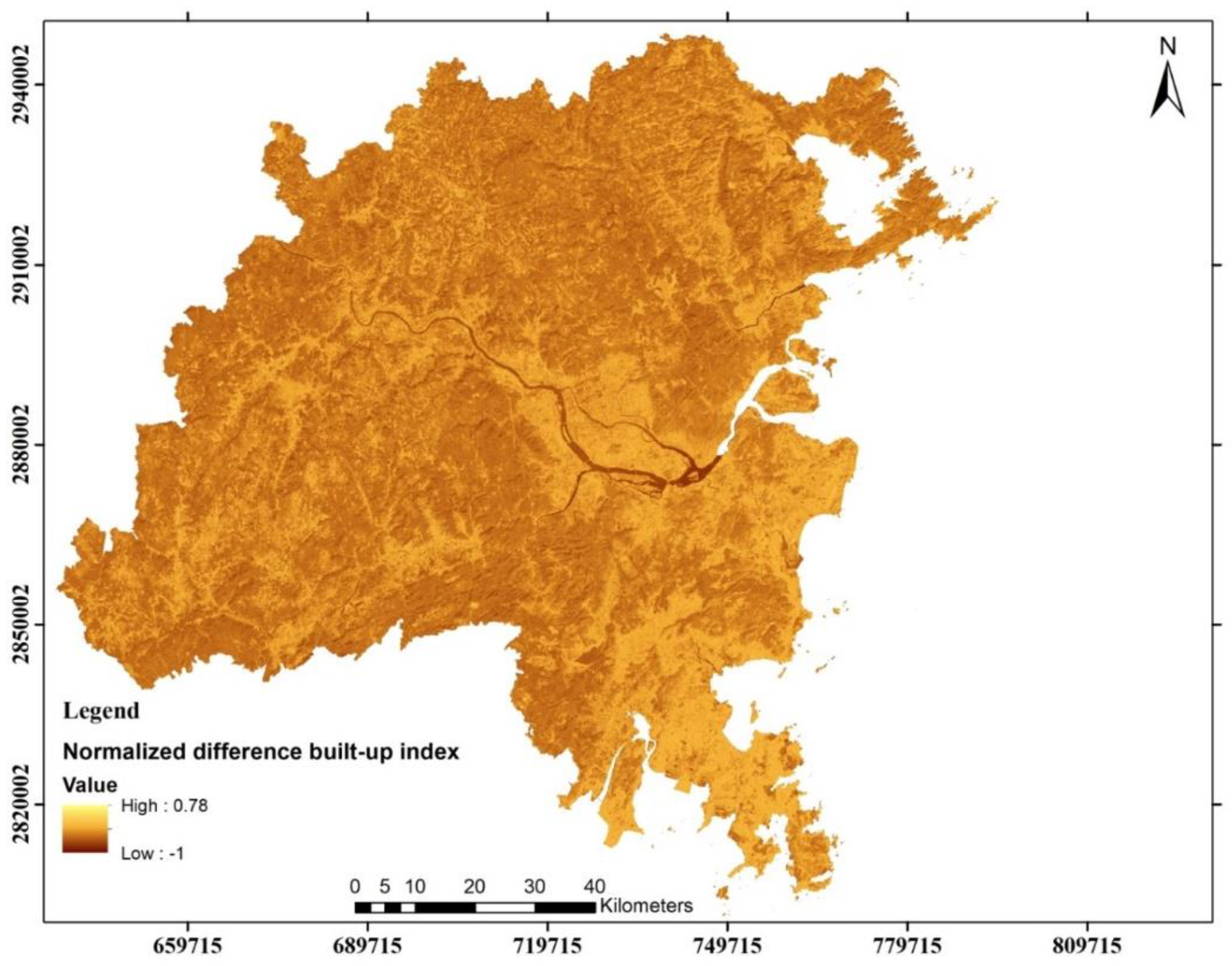
| Normalized difference built-up index | [20] | |
| Topographic position index (TPI) | [21] | |
| Greenness index | [22] | |
| Curvature | [23] | |
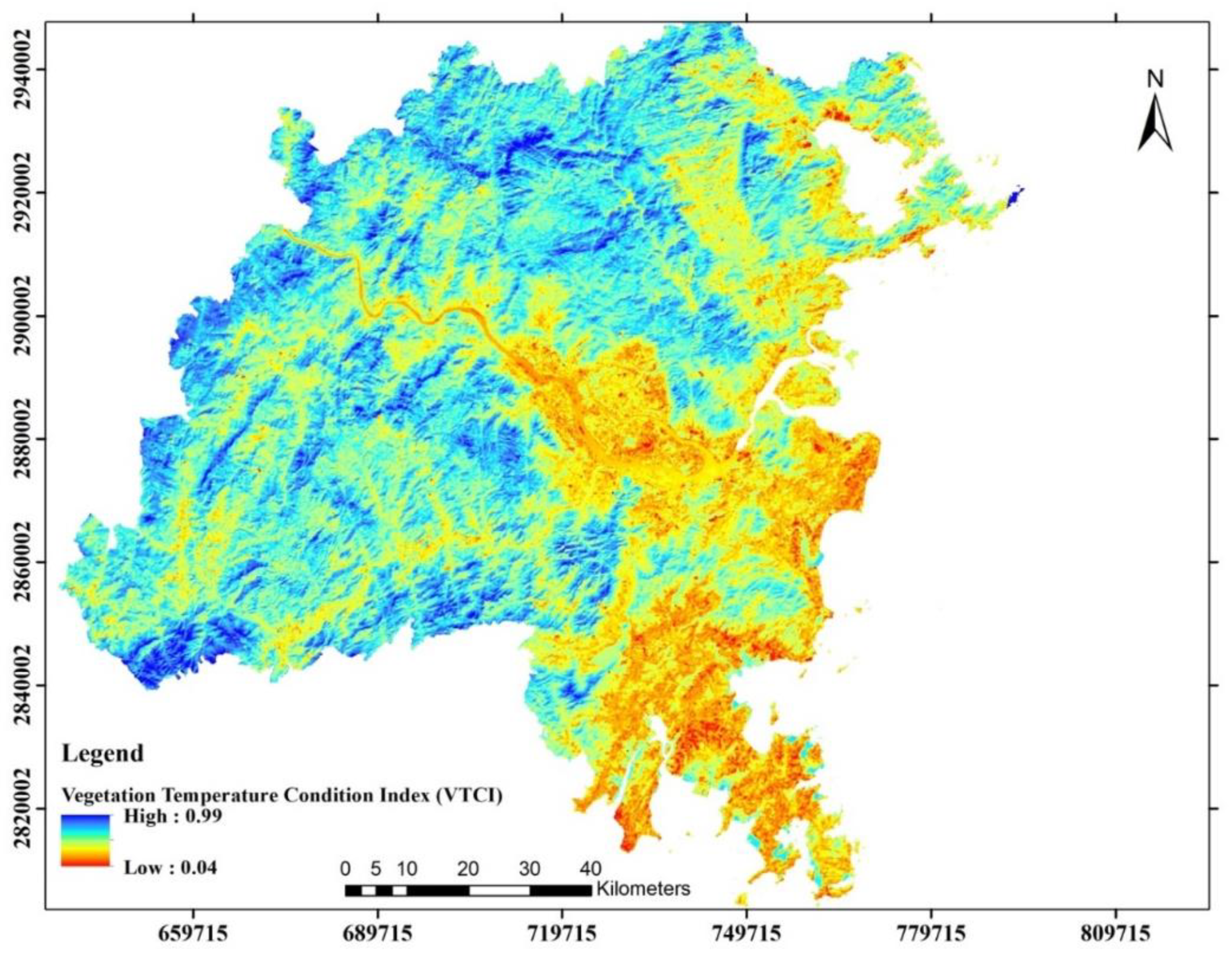
| Vegetation temperature condition index | [24] | |
| Proportion of Vegetation | [25] | |
| Adjusted transformed soil-adjusted Vegetation Index | [25] | |
| Emissivity | [25] | |
| Soil-adjusted vegetation index | [26] | |
| Aspect | [27] | |
| Normalized difference vegetation index | [28] | |
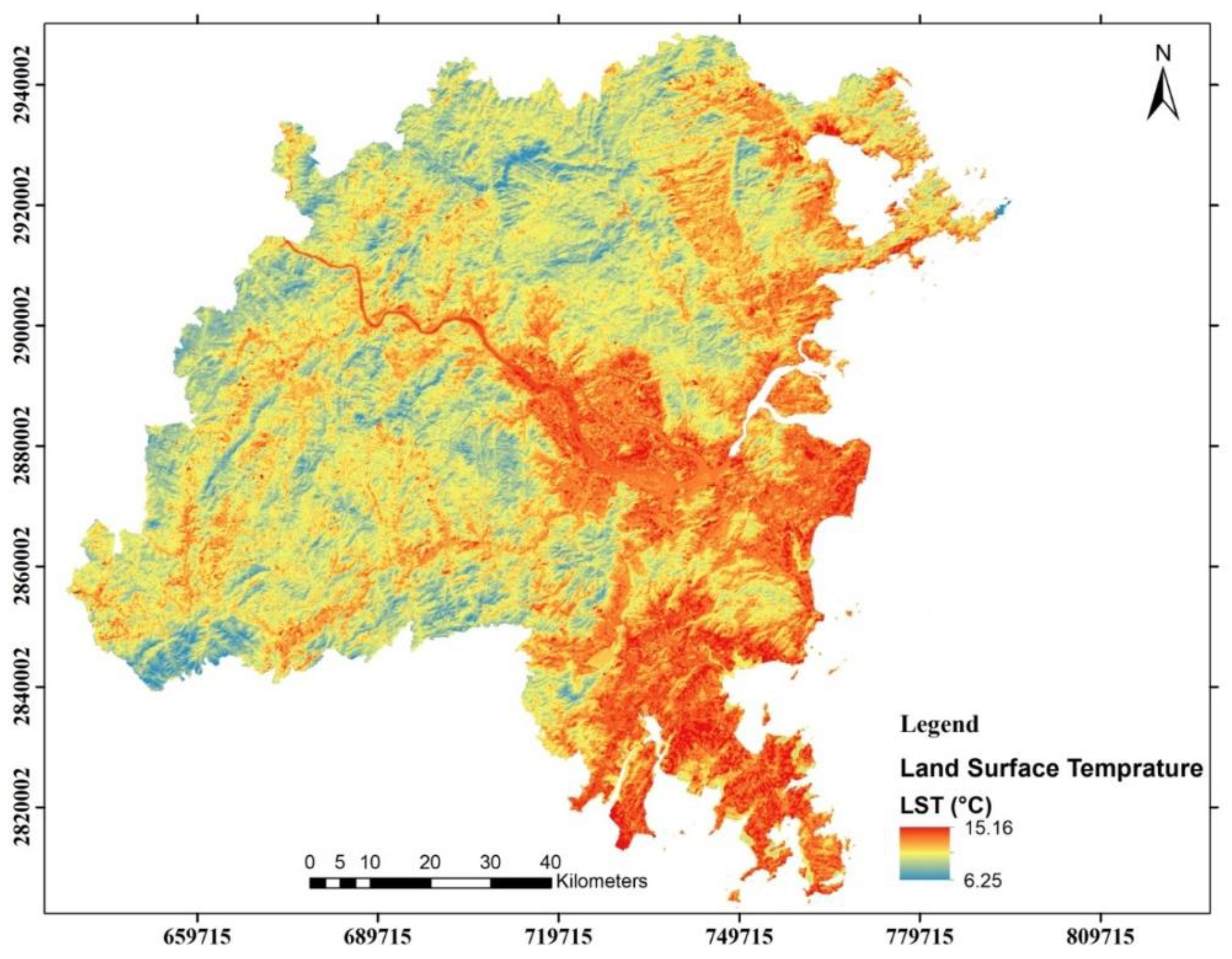
| Land surface temperature | [29] | |
| Profile curvature | [30] | |
| Brightness temperature | [25] | |
| Slope | [31] | |
| Enhanced vegetation index | [28] | |
| Brightness index | [22] | |
| Wetness index | [32] | |
| Mass balance index | [33] | |
| Topographic wetness index | [34] | |
| Length slope (LS) factor | [35] | |
| Thiam’s transformed vegetation index | [36] | |
| Corrected transformed vegetation index | [37] | |
| Normalized ratio vegetation index | [38] | |
| Normalized ratio vegetation index | [38] | |
| Ratio vegetation index | [38] | |
| Difference vegetation index | [39] | |
| Transformed soil-adjusted vegetation index (Baret and Guyot, 1991) | 2) | [40] |
| Transformed soil-adjusted vegetation index (Baret et al. 1989) | [26] | |
| Perpendicular vegetation index (Perry and Lautenschlager, 1984) | [41] | |
| Perpendicular vegetation index (Qi, et al-, 1994) | [41] | |
| Perpendicular vegetation index (Richardson and Wiegand, 1977) | [42] | |
| Distance from industries, landfill | DST_Inds = proximity analysis | [43] |
| Distance from primary roads | DST_PR = proximity analysis | [43] |
| Distance from water bodies, canal, dam, ditch, drain, riverbank, river, stream, waterfall, weir | DST_RCD = proximity analysis | [43] |
| Aerosol band 1 | Coastal aerosol (0.443 µm) | [44] |
| Blue band | Blue (450–510 nm) | [44] |
| Green band | Green (530–590 nm) | [44] |
| Red band | Red (640–670 nm) | [44] |
| NIR band | Near infrared (NIR) (850–880 nm) | [44] |
| SWIR-1 band | SWIR-1 (1570–1650 nm) | [44] |
| SWIR-2 band | SWIR-2 (2110–2290 nm) | [44] |
| Land-use types | Supervised the maximum-likelihood method | [45] |
| Landform types | TPI-based landform classification | [21] |
| Soil pH | pH meter | |
| Lithology | FAO soil database | |
| Spectral soil data | Wavelength (from 350 to 2500 nm with 1 nm interval) |
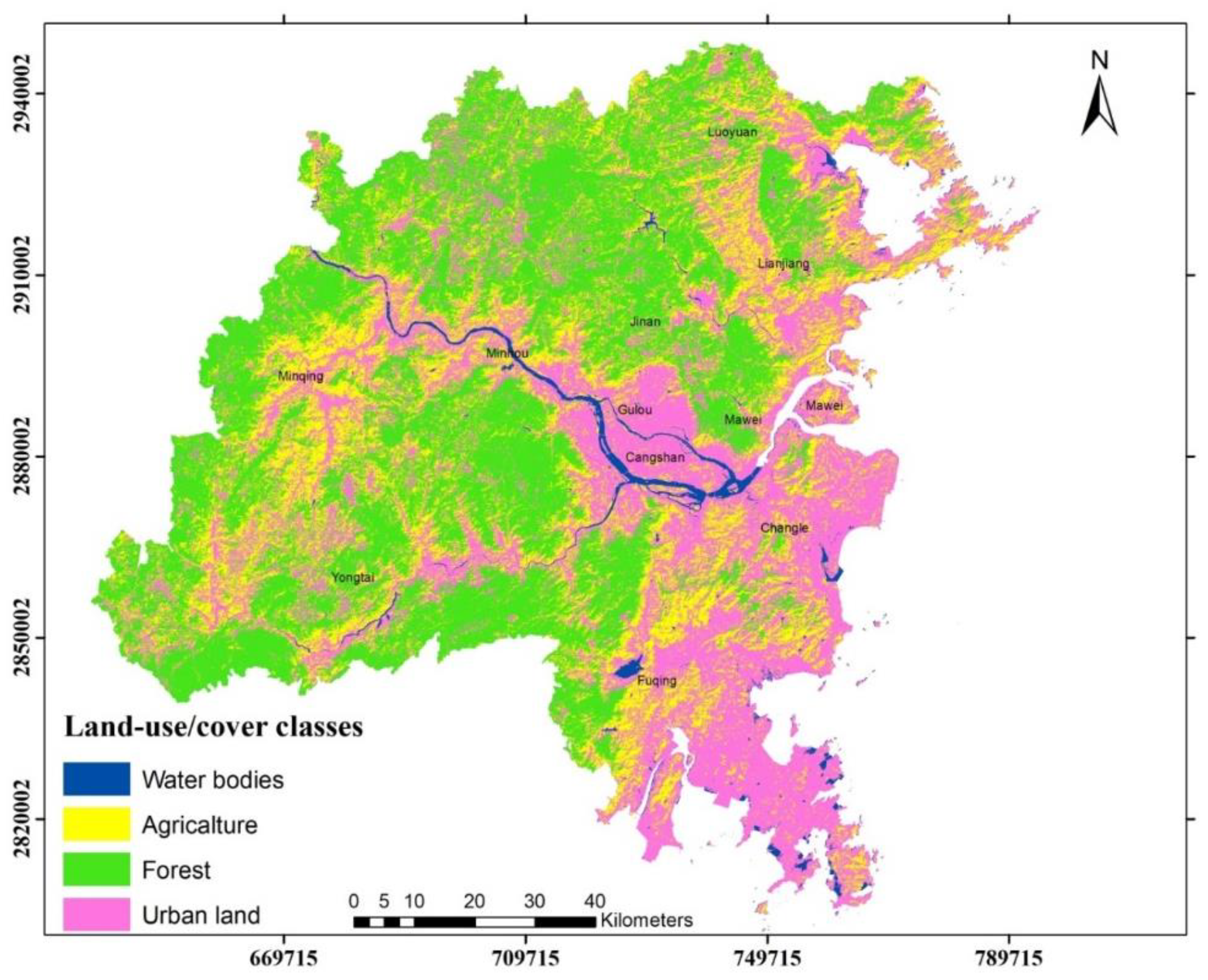
| Main Land Cover | Area (ha) | Area Proportion (%) | Com. Error | Om. Error | Acc. |
|---|---|---|---|---|---|
| Agriculture | 28,198.71 | 21.80 | 3.04 | 0.58 | |
| Forest | 44,562.51 | 34.44 | 2.13 | 0.74 | 95.52 |
| Water bodies | 18,580.59 | 14.36 | 0.15 | 0.38 | |
| Urban land | 38,034.36 | 29.40 | 1.2 | 3.08 |
| Datasets | Indicators | Min | 25% | Mean | 75% | Max. | SD |
|---|---|---|---|---|---|---|---|
| Training set | ME | 0.05 | 0.04 | 0.04 | 0.03 | 0.06 | 0.003 |
| RMSE | 1.35 | 1.36 | 1.37 | 1.37 | 1.38 | 0.026 | |
| R2 | 0.68 | 0.76 | 0.033 | ||||
| Test set | ME | 0.3 | 0.4 | 0.4 | 0.43 | 0.36 | 0.001 |
| RMSE | 0.94 | 0.95 | 0.96 | 0.96 | 0.97 | 0.024 | |
| R2 | 0.88 | 0.91 | 0.92 | 0.021 |
| Variables (Unit) | Min. | Max. | Mean | zSD | CV | yr | L.B. | U.B. | Coeff. | p−Values | R2 |
|---|---|---|---|---|---|---|---|---|---|---|---|
| SOC (mg·g−1) | 0.70 | 45.80 | 11.70 | 8.92 | 0.81 | 1 | - | - | - | - | - |
| Slope (°) | 0.00 | 103.51 | 37.55 | 23.55 | 0.58 | −0.16 | −0.33 | 0.02 | 0.02 | 0.09 | 0.03 |
| Curvature | −5.80 | 5.94 | 0.22 | 2.11 | 0.36 | −0.19* | −0.36 | −0.01 | 0.04 | 0.04 | 0.04 |
| Aspect | −1.00 | 357.92 | 160.70 | 117.89 | 0.67 | 0.16 | −0.02 | 0.33 | 0.03 | 0.08 | 0.03 |
| TPI | −2.29 | 2.10 | −0.01 | 0.93 | 0.41 | 0.10 | −0.08 | 0.27 | 0.01 | 0.29 | 0.01 |
| MBI | −0.84 | 0.87 | 0.06 | 0.54 | 0.61 | −0.18* | −0.35 | 0.00 | 0.03 | 0.05 | 0.03 |
| TWI | −1.95 | 11.55 | 6.79 | 3.66 | 0.43 | 0.17 | −0.01 | 0.34 | 0.03 | 0.06 | 0.03 |
| LS Factor | 0.00 | 21.791 | 10.633 | 7.473 | 0.68 | −0.06 | −0.23 | 0.12 | 0.68 | 0.96 | 0.01 |
| NDVI | −0.47 | 0.89 | 0.64 | 0.24 | 0.19 | 0.20* | −0.36 | −0.02 | 0.04 | 0.03 | 0.04 |
| ASTAVI | −0.70 | 1.35 | 0.96 | 0.35 | 0.18 | 0.23* | −0.39 | −0.05 | 0.05 | 0.01 | 0.05 |
| WI | 0.01 | 0.21 | 0.11 | 0.04 | 0.39 | −0.14 | −0.31 | 0.04 | 0.02 | 0.13 | 0.02 |
| GI | −0.09 | 0.27 | 0.12 | 0.08 | 0.35 | 0.28* | −0.44 | −0.11 | 0.08 | 0.00 | 0.08 |
| BI | 0.02 | 0.39 | 0.20 | 0.07 | 0.40 | −0.11 | −0.28 | 0.07 | 0.01 | 0.23 | 0.01 |
| EVI | −0.07 | 0.55 | 0.29 | 0.15 | 0.38 | 0.28* | −0.43 | −0.10 | 0.08 | 0.00 | 0.08 |
| SAVI | −0.48 | 1.13 | 0.78 | 0.29 | 0.20 | 0.24* | −0.40 | −0.07 | 0.06 | 0.01 | 0.06 |
| CTVI | 0.42 | 1.12 | 1.00 | 0.11 | 0.16 | 0.22* | −0.39 | −0.05 | 0.05 | 0.01 | 0.05 |
| TVI | 0.09 | 1.37 | 1.21 | 0.17 | 0.28 | 0.22* | −0.38 | −0.04 | 0.05 | 0.01 | 0.05 |
| NRVI | −0.32 | 0.76 | 0.52 | 0.19 | 0.20 | 0.24* | −0.40 | −0.07 | 0.06 | 0.01 | 0.06 |
| RVI | 0.51 | 7.18 | 3.77 | 1.61 | 0.46 | 0.27* | −0.43 | −0.10 | 0.07 | 0.00 | 0.07 |
| TSAVI_91 | 0.01 | 0.73 | 0.53 | 0.15 | 0.25 | 0.26* | −0.42 | −0.08 | 0.07 | 0.00 | 0.07 |
| PV | 0.00 | 0.59 | 0.05 | 0.08 | 1.68 | 0.14 | −0.04 | 0.31 | 0.02 | 0.13 | 0.02 |
| LST (°C) | 6.25 | 15.15 | 10.65 | 2.11 | 0.47 | 0.09 | −0.09 | 0.27 | 0.01 | 0.32 | 0.01 |
| VTCI | 0.04 | 0.99 | 0.51 | 0.23 | 0.48 | 0.09 | −0.09 | 0.27 | 0.01 | 0.32 | 0.01 |
| NDBI | −0.65 | 0.07 | −0.30 | 0.16 | 0.44 | 0.26* | 0.08 | 0.41 | 0.07 | 0.00 | 0.07 |
| DST_INDST (km) | 1.05 | 62.59 | 16.35 | 12.15 | −0.12 | −0.29 | 0.06 | 0.01 | 0.20 | 0.01 | |
| DST_PR (km) | 0.07 | 43.64 | 9.77 | 9.01 | 0.88 | −0.05 | −0.23 | 0.12 | 0.00 | 0.55 | 0.00 |
| DST_RCD (km) | 0.04 | 25.05 | 3.38 | 4.92 | 1.46 | −0.13 | −0.31 | 0.05 | 0.02 | 0.14 | 0.02 |
| Band2 | 824.94 | 1552.34 | 1057.66 | 172.56 | 0.70 | 0.16 | −0.02 | 0.33 | 0.03 | 0.08 | 0.03 |
| Band3 | 496.94 | 1503.39 | 826.82 | 213.15 | 0.61 | 0.10 | −0.08 | 0.28 | 0.01 | 0.25 | 0.01 |
| Band4 | 308.63 | 1526.16 | 647.02 | 270.15 | 0.77 | 0.13 | −0.04 | 0.31 | 0.02 | 0.14 | 0.02 |
| Band5 | 404.82 | 3859.93 | 2202.38 | 780.76 | 0.42 | −0.23* | −0.39 | −0.05 | 0.05 | 0.01 | 0.05 |
| Band6 | 123.38 | 2683.87 | 1230.17 | 543.24 | 0.50 | −0.02 | −0.19 | 0.16 | 0.00 | 0.87 | 0.00 |
| Band7 | 54.04 | 1817.46 | 671.75 | 397.67 | 0.64 | 0.09 | −0.09 | 0.26 | 0.01 | 0.35 | 0.01 |
| pH | 0.00 | 9.10 | 4.82 | 1.81 | 0.38 | 0.12 | −0.06 | 0.29 | 0.01 | 0.19 | 0.01 |
| Landform | Min | Max | Mean | SD | CV (%) |
|---|---|---|---|---|---|
| TM | 3.70 | 34.06 | 12.64 | 8.52 | 67.43 |
| LP | 1.65 | 29.47 | 11.94 | 6.78 | 56.79 |
| SH | 0.70 | 45.80 | 11.88 | 9.28 | 78.09 |
| SM | 2.29 | 26.24 | 10.90 | 13.31 | 122.08 |
| TH | 1.70 | 1.70 | 1.70 | - | - |
| WR | 3.83 | 11.12 | 7.48 | 5.15 | 68.96 |
| Land Use | Min | Max | Mean | SD | CV (%) |
|---|---|---|---|---|---|
| Agriculture | 0.70 | 39.57 | 10.43 | 8.37 | 80 |
| Forestland | 1.65 | 45.80 | 13.60 | 8.49 | 62 |
| Urban area | 1.70 | 26.5 | 9.74 | 9.83 | 101 |
| Water bodies | 0.6 | 8.89 | 4.55 | 5.86 | 129 |
| Lithology | Min | Max | Mean | SD | CV (%) |
|---|---|---|---|---|---|
| Pyroclastic, ignimbrite | 1.34 | 45.80 | 12.04 | 9.73 | 80.80 |
| Sandstone, greywacke, arkose | 1.70 | 14.27 | 5.54 | 4.53 | 81.80 |
| Fluvial | 2.63 | 29.47 | 13.57 | 9.97 | 73.51 |
| Gneiss, migmatite | 0.70 | 31.47 | 11.91 | 8.61 | 72.30 |
| Granite | 4.39 | 15.24 | 11.61 | 4.98 | 42.87 |
| Shale | 3.70 | 34.06 | 14.52 | 9.58 | 65.98 |
| Siltstone, mudstone, claystone | 1.65 | 12.03 | 7.93 | 4.45 | 56.14 |
| Inland water or lakes deposits | 3.83 | 11.12 | 7.48 | 5.15 | 68.96 |
| Marine unconsolidated rock | 8.73 | 13.26 | 11.00 | 3.20 | 29.10 |
| Weathered residuum, bauxite, laterite | 2.12 | 35.67 | 14.69 | 11.06 | 75.30 |
Publisher’s Note: MDPI stays neutral with regard to jurisdictional claims in published maps and institutional affiliations. |
© 2021 by the authors. Licensee MDPI, Basel, Switzerland. This article is an open access article distributed under the terms and conditions of the Creative Commons Attribution (CC BY) license (https://creativecommons.org/licenses/by/4.0/).
Share and Cite
Sodango, T.H.; Sha, J.; Li, X.; Noszczyk, T.; Shang, J.; Aneseyee, A.B.; Bao, Z. Modeling the Spatial Dynamics of Soil Organic Carbon Using Remotely-Sensed Predictors in Fuzhou City, China. Remote Sens. 2021, 13, 1682. https://doi.org/10.3390/rs13091682
Sodango TH, Sha J, Li X, Noszczyk T, Shang J, Aneseyee AB, Bao Z. Modeling the Spatial Dynamics of Soil Organic Carbon Using Remotely-Sensed Predictors in Fuzhou City, China. Remote Sensing. 2021; 13(9):1682. https://doi.org/10.3390/rs13091682
Chicago/Turabian StyleSodango, Terefe Hanchiso, Jinming Sha, Xiaomei Li, Tomasz Noszczyk, Jiali Shang, Abreham Berta Aneseyee, and Zhongcong Bao. 2021. "Modeling the Spatial Dynamics of Soil Organic Carbon Using Remotely-Sensed Predictors in Fuzhou City, China" Remote Sensing 13, no. 9: 1682. https://doi.org/10.3390/rs13091682
APA StyleSodango, T. H., Sha, J., Li, X., Noszczyk, T., Shang, J., Aneseyee, A. B., & Bao, Z. (2021). Modeling the Spatial Dynamics of Soil Organic Carbon Using Remotely-Sensed Predictors in Fuzhou City, China. Remote Sensing, 13(9), 1682. https://doi.org/10.3390/rs13091682