Abstract
Remote sensing image object detection has been studied by many researchers in recent years using deep neural networks. However, optical remote sensing images contain many scenes with small and dense objects, resulting in a high rate of misrecognition. Firstly, in this work we selected a deep layer aggregation network with updated deformable convolution layers as the backbone to extract object features. The detection and classification of objects was based on the center-point network without non-maximum suppression. Secondly, the dynamic gradient adjustment embedded into the classification loss function was put forward to harmonize the quantity imbalance between easy and hard examples, as well as between positive and negative examples. Furthermore, the complete intersection over union (CIoU) loss function was selected as the objective function of bounding box regression, which achieves better convergence speed and accuracy. Finally, in order to validate the effectiveness and precision of the dynamic gradient adjustment network (DGANet), we conducted a series of experiments in remote sensing public datasets UCAS-AOD and LEVIR. The comparison experiments demonstrate that the DGANet achieves a more accurate detection result in optical remote sensing images.
1. Introduction
With the rapidly developing technology applied in the remote sensing field, target detection in remote sensing images has been a popular area of research because of its wide applications [1,2,3,4,5]. Meanwhile, object detection in optical remote sensing is faced with various challenges, including changes in the appearance of objects caused by illumination, observation angle, shadow, weather, and partial shelter. These challenges result in a relatively lower accuracy and higher computational complexity compared with general object detection methods. In recent years, deep convolution neural networks (CNNs) have been used by researchers to detect objects, and a variety of methods have been proposed to achieve better performance [6,7,8,9,10,11,12,13,14]. The excellent performance of CNN arouses the research interest of scholars. Detection methods based on CNN have been applied in fields such as image denoising, object detection, semanteme division, pose estimation, and object tracking in natural scene images [15,16,17,18]. Meanwhile, some improved CNN methods have been applied in optical remote sensing images to promote performance and applicability [1,19,20,21]. Besides, a new set of methods based on Capsule network are proposed for object detection [22,23,24,25,26], which may offer another alternative solution for optical remote sensing images as an emerging research area.
In general, typical deep convolutional neural networks can be divided into anchor-based and anchor-free according to the regression of bounding box. For the anchor-based framework, the regression of the bounding box relies on a set of pre-defined anchor boxes with various sizes and aspect ratios. Detect networks such as Faster R-CNN [27], SSD [14], YOLOv2 [28] and YOLOv3 [29] are of the anchor-based framework. This type of method needs to select a certain number of anchor boxes on the feature layer, then it calculates the confidence of objects and refines bounding boxes according to the intersection over union (IoU), and finally draws detection results including these refined bounding boxes and confidences on original images. However, the use of the anchor box suffers from two drawbacks. First, the network needs a certain number of preset anchor boxes to match different objects with various scales and aspect ratios, while most of the preset boxes are invalid that would increase the training time of the model [30]. Second, the anchor-based method introduces many hyper-parameters that need to be optimized [14,30], which increases the difficulty of model design.
Due to the emergence of Feature Pyramid Networks [31] and Focal Loss [30], some scholarly research has been performed to investigate anchor-free network frameworks. The networks directly detect objects without presetting anchor boxes, which is conducive to the design of the network and the improvement of training speed. Anchor-free detectors can be divided into two different types. The first type delineates the bounding box by merging a pair of corner points of the target. This kind of anchor-free detector, such as CornerNet [32,33] and MatrixNets [34], is classified as the keypoint-based network. The other type locates the center point of the targets and then predicts the width and height of the bounding box. This kind of anchor-free detector is called a centerpoint-based network [35,36]. The CenterNet [35] doesn’t need to preset a large number of anchor boxes and has achieved similar or even better performance compared with anchor-based detectors. Centerpoints appear inside the object while corners are outside, so the extraction of centerpoints is more accurate. The centerpoint-based detectors have more advantages in object detection.
Focal Loss is used to solve the class imbalance between foreground and background as well as between easy and hard examples. However, Li et al. [37] points out that Focal Loss defines a static ratio coefficient to increase attention to hard examples during training, which does not adapt the change of data distribution. In this context, the article propose a gradient harmonizing mechanism (GHM) to restrict the disharmony. In the field of remote sensing, there is a large number of hard examples in remote sensing images because of illumination, shadow, shelter, haze and so on. Referring to the experimental results, we define these indistinguishable examples as outliers because they exist stably even after the model is converged. The schematic diagram of outliers is shown in Figure 1. We introduce the gradient harmonizing method into the Centernet to improve the performance of the model. However, the gradient harmonizing mechanism doesn’t consider the imbalance between positive examples and negative examples, and the inhibition mechanism of example imbalance needs to be further improved.
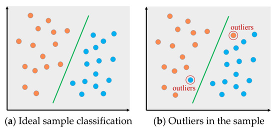
Figure 1.
Illustrations of object classification in deep learning, Colors are used to distinguish different catagories of objects. (a) Under ideal conditions. (b) Outliers in the sample.
We propose a dynamic gradient adjustment anchor-free object detection method used for optical remote sensing field. The model is based on CenterNet [36], and the deep layer aggregation [38] combined with deformable convolution layers [39] was chosen as the backbone network to extract effective features of objects. In order to settle the problem of example imbalance and improve the performance of the detector, we propose a dynamic gradient adjustment network which embeds the gradient density into the updated Focal Loss function. Furthermore, the Complete-IoU loss function [40] is used for the regression of bounding box, which can harmonize the coupling characteristic of border size and its location. Contrast experiments were conducted to compare the performance of the proposed method with other advanced detectors on dataset UCAS-AOD and LEVIR. The experimental results show that the proposed network significantly improves the accuracy of object detection.
The main contributions of this article are listed as follows:
- We propose a dynamic gradient adjustment method to harmonize the quantity imbalance between easy and hard examples as well as between positive and negative examples.
- For the detection of small and dense objects in optical remote sensing images, we select a deep layer aggregation combined with deformable convolution as the backbone network, which has a better prediction performance.
- We select the Complete-IoU as regression loss function instead of the sum of dimension loss and position offset loss to improve learning efficiency.
- The object detection precision and recall in optical remote sensing images demonstrate the significant improvement of our method.
The rest of the article is organized as follows. Section 2 reviews relevant works in remote sensing object detection and describes basic principles of CenterNet. We expound the proposed improved method in Section 3. The effectiveness of the proposed method is verified and comparison experiments with the existing detectors are conducted in Section 4. Finally, Section 5 gives the conclusion of this article.
2. Related Work
2.1. Object Detection in Remote Sensing Images
With the continuous development of deep learning techniques, some of the latest networks take object detection as a classification problem and prediction performance is constantly being improved. Simultaneously, many approaches have been introduced into the optical remote sensing field, where detection faces more complex challenges. Chen et al. proposed a hybrid CNN for vehicle detection in satellite images [41]. This method was capable of extracting multi-scale features at its highest convolutional layer, which could improve the separability of the space feature. But the method cannot be used for multi-target recognition because it selected a time-consuming sliding-windows search paradigm to locate targets. Singular Value Decompensation Networks (SVDNet) was proposed [42] to generate candidate objects through convolution layers and nonlinear mapping layers. Then it further verified each candidate by using feature pooling and the linear SVM classifier. But the dependence on prior knowledge limited its application expansion. Han et al. proposed an object detection method based on the classical paradigm Faster R-CNN, which improved the effectiveness and robustness by sharing features between the region proposal generation stage and the object detection stage [43]. In order to improve the accuracy of Faster R-CNN, authors [44] introduced dilated convolution, multi-scale combination and Online Hard Example Mining (OHEM) [45] into the network. Besides, this method used a fully convolution neural network instead of the fully connected layer to realize the lightweight of model. In order to detect small objects under complex background conditions, scholars proposed an object detection method based on multi-attention, which identified a global spatial attention module to pay attention to the location of objects and reduced the loss of small items [46]. However, the performance and the real-time function of those methods need to be further improved.
2.2. Development and Basic Principle of CenterNet
With the emergence of Feature Pyramid Networks [31] and Focal Loss [30], the detectors based on the anchor-free network become a research hotspot and exhibit their good performance. CornerNet [32] was first reported in 2018 and realized anchor-free detection by regarding the object as a pair of corner points. Authors designed two heatmap branches to predict the top-left corner point and bottom-right corner point, respectively. In order to settle the problem of no local visual feature for the location of corners, the corner pooling module was proposed. The detector achieved the highest detection accuracy at that time. Inspired by CornerNet, Keypoint Triplets [35] detected top-left corner, bottom-right corner and center point of the object as triplets, while ExtremeNet [47] detected the top-most, left-most, bottom-most, right-most, and center point of the object. Both these methods build on the same robust keypoint estimation network. However, they require a combinatorial grouping stage after keypoint detection, which significantly reduces the detection speed.
CenterNet simply extracted the center-point for each object, and then regressed the size and the location of the bounding box. The input image was feed into a Fully Convolution Network to generate a heatmap branch, in which peaks corresponded to target centers. Offset branch predicted the location offsets of the center pixel while size branch predicted the height and weight of the bounding box. CenterNet assigned anchor based on center point, while adjacent points were lowered in sequence, thus there was no need to set thresholds between foreground and background classification. The recognition speed of CenterNet was much better than that of anchor-based detectors, since it eliminated the need for multiple anchors.
3. Proposed Approach
In our proposed approach, the Centernet [36] is used as our baseline, and the framework of the dynamic adjustment network is shown in Figure 2. The detection regards the object as a point and then regress the size and offset of bounding box. The deep convolution network extracts features of the input image and generates a heatmap. Peaks in the heatmap indicate detected objects. Due to the influence of light, obscuration and sharpness, images contain a few objects that are difficult to distinguish. We call them outliers. Dynamic gradient adjustment module is proposed to dynamically refine the loss weight depend on density distribution and minimize the effect of these outliers.
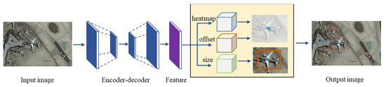
Figure 2.
The framework of the dynamic adjustment network. Dynamic gradient adjustment (DGA) module dynamically refine the prediction of heatmap.
Deep Layer Aggregation (DLA34) [38] is used as the backbone network of the model, which is illustrated in Figure 3. The upgraded deformable convolutional net (DCN) is used as up sampling to connect features between layers in the network. The shallow layer has spatial-rich information and is more advantageous to detect small targets, while deep layer with semantic-rich information has better robustness and is more suitable for detecting large targets. This approach realizes multi-scale feature fusion and effectively extracts the feature information of objects at different scales. Besides, we introduce the CIoU to improve the convergence speed and accuracy of the model.
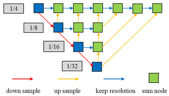
Figure 3.
Illustrations of the DLA34 backbone network. The deformable convolutional layer is used for up sample instead of common inverse convolution in deep layer aggregation.
3.1. Dynamic Gradient Adjustment for Classification Function
This region is focused on classification in anchor-free object detection where the class (foreground and background) of images, as well as easy and hard examples, are quite imbalanced. Concerning this issue, we propose a dynamic refinement mechanism to inhibit these two disharmonies based on updated Focal Loss and GHM. Both of them originate from the multi-classification cross entropy loss:
In Equation (1), denotes the ground-truth label for a certain class and is the probability predicted by the detector.
Experiments show that the large class imbalance, as well as disharmony between easy and hard examples, limits the improvement of detector performance. We propose the dynamic gradient adjustment focal loss to settle the problem:
The input image is defined as with width and height . The detector extracts the targets as points, and then maps all ground truth keypoints onto a heatmap . indicates the number of classes, while is the down-sampling factor of the network. The heatmap is expected to be equal to 1 at target centers and adjacent positions are decreasing in order. The values on the heatmap are not less than 0. Refering to the practice of CornerNet [32] and CenterNet [36], the ground truth center points of targets are mapped using a 2D Gaussian kernel , where and are the target center points after down-sampled, while is a standard deviation which changes with the size of the object. In Equation (2), is used to harmonize positive and negative examples, while and are hyper parameters of the updated Focal Loss, respectively. N is the number of center-points in an image, and it is applied to normalize all positive focal losses instance to 1.
Meanwhile, in Equation (2) is introduced to dynamically refine the loss function by reducing weight of easy examples and hard examples. GHM adds the in Equation (1) to improve the performance of one-stage detectors. Gradient density and gradient norm are defined as follows:
In Equation (3), is the gradient norm of the k-th example, and is a function indicating whether is located in the interval centered at with a valid length .
Thus, gradient density GD(g) represents the ratio of examples in the specific interval to all examples. It is a dynamically varying value determined by predictions. is used to down-weights the contribution of outliers as well as easy examples.
3.2. United Bounding Regression Function
The regression loss function of the bounding box in CenterNet is defined as , where denotes the loss function of the bounding box size by using the L1 loss and is introduced to inhibit the discretization error of the center-point caused by the output stride. However, there are two drawbacks to this approach. First, the size and location of the bounding box are regarded as two independent variables, which violated the fact that the size and location of an object are highly correlated. Second, this method introduces weight parameters and , which need to be optimized. We select the CIoU as the bounding box regression function and its schematic diagram is shown in Figure 4.
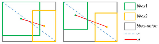
Figure 4.
Illustrations of complete-intersection over union (CIoU) loss for bounding box regression. c is the diagonal length of the smallest enclosing box covering bbox1 and bbox2, and d is distance of center-points of two boxes. Besides, additional is the parameter of aspect ratio.
The united regression function is defined as follows:
where and denote the center-points of predicted bounding box and ground truth bounding box, respectively. is the maximal overlap between the predicted bounding box and the ground truth box. is the Euclidean distance of two points and is the diagonal length of the smallest enclosing box that covers the predicted box and ground truth box. is a positive trade-off parameter and measures the consistency of box aspect ratio. Besides, Distance IoU (DIoU) is defined similarly to CIoU, which doesn’t consider the effect of aspect ratio. Since the experiment part involves the comparison of both of the methods, the expression of DIoU is given here:
After a series of optimizations to the classification function and regression function, the overall training objective is:
and are equal to 1 in our experiments. DGANet is used to predict the center-point, offset, and size of objects. All output branches share a common fully convolution backbone network as shown in Figure 2.
4. Experiment and Discussion
In the experimental section, we describe a series of experiments conducted to demonstrate the effectiveness of the proposed network in optical remote sensing images. First, we introduce datasets used and evaluation metrics for the performance. Second, we describe four groups of experiments conducted to evaluate the performance of the proposed DGANet. Finally, we compare the method with published state-of-the-art approaches to adequately prove the advantages of our DGANet framework.
4.1. Datasets and Evaluation Metrics
UCAS-AOD: Ablation experiments are conducted on an dataset named UCAS-AOD [48] with two commonly used categories: car and plane. The airplane category is composed of 1000 optical remote sensing images with 7482 objects in total. In contrast, the car category is composed of 510 optical remote sensing images with 7114 items in total. The dataset sequence is randomly arranged. For the training set 80% of figures were randomly chosen, while the rest were adopted as the validation set.
LEVIR: The LEVIR dataset [49] is selected from high-resolution Google Earth images with more than 22 thousand images. The dataset background covers most types of geomorphic features such as city, country, mountain area, and ocean. There are three categories of objects: airplane, ship (inshore and offshore ships), and oil-tank, respectively. It contains 11 thousand labeled images, including 4724 airplanes, 3025 ships, and 3279 oil-tanks for training. In contrast, 6585 images are set as the validation set.
Experiments were performed on a laptop with an Intel single Core i7 Central Processing Unit (CPU), NVIDIA RTX-2070 GPU (8 GB memory). The deep learning operating environment is Pytorch 1.2.0, CUDA 10.0, Python version 3.6. The initial learning rate was set to 1.25e-4, and the batch size was set to 8.
Evaluation metrics: We selected two widely used indicators mean Average Precision (mAP) and mean Recall (mRecall) to measure the performance of different frameworks of detectors. The evaluation method [50] is described as follows:
- IoU: Intersection-over-union (IoU) is used to describe the matching rate between the ground truth box and the predicted box. If the calculated value of IoU is higher than the threshold, the predicted result is labeled as true positive (TP); otherwise it is annotated as false positive (FP). If a ground truth box does not been matched by any predicted box, it is regarded as an false negative (FN).
- Precision and recall: precision and recall are obtained by calculating the number of TP, FP, and FN.
Precision and recall are important indexes of model evaluation, and they can be used to evaluate a certain category.
- 3.
- Average precision: Average precision (AP) corresponds to a certain category to calculate the mean value of precision for each recall rates, and it is a comprehensive index sensitive to sort. mAP is the calculated average value of each AP. Meanwhile, mRecall is the mean value of the recall for all classes. We adopted the mAP and mRecall at the IoU threshold of 0.5 to evaluate the performance of the detector. In addition, the objects are divided into three categories by area. Intervals of instance area are (1 × 1, 32 × 32), (32 × 32, 96 × 96), and (96 × 96, inf), corresponding to “small”, “medium”, and “large” respectively. The mean average precisions from IoU = 0.5 to IoU = 0.95 with step size of 0.05 for each group were defined as APS, APM, and APL.
4.2. Ablation Experiments
A series of contrast experiments were conducted to verify the superiority of our proposed approaches. In order to make it more intuitive, we defined ORIG to denote the baseline model CenterNet [36]. The ablation experiments cover the evaluation of the dynamic gradient adjustment (DGA) and the united bounding regression (UBR), as well as their combination DGANet.
4.2.1. Evaluation of Dynamic Gradient Adjustment
In order to verify the superiority of DGA module, we conducted multiple sets of experiments to compare the performance among the original CenterNet and different DGA frameworks. Table 1 shows some of the main contrast results of different classification modules. First, we introduced an equilibrium coefficient to address the imbalance between positive and negative examples. The parameter was introduced to avoid overlearning easy negative examples that contribute little to the detector, which was set to 0.25 after a series of experiments. A comparison of the results between ORIG and DGA-1 revealed that mAP increased from 0.942 to 0.961 with an increase of 1.9 percent.

Table 1.
Performance comparison among different setting of classification modules used on the UCAS-AOD dataset. mAP, mean Average Precision; mRecall, mean Recall; GD, gradient density; ORIG, baseline model CenterNet.
Second, gradient density was used to dynamically refine the Focal Loss function to harmonize the imbalance easy and hard examples. DGA-2 stands for the updated gradient harmonizing mechanism, which introduces two hyper-parameters and to improve the recognition ability of the model to real samples. We have designed verification experiments and obtained positive results. When hyper-parameters were equal to 0, the performance of the detector degraded, and the prediction accuracy of GDA-3 deteriorated to 0.927. DGA-4 defines as equal to 4, and the mAP reached 0.952, which achieves 2.5% higher than DGA-3 and 1% higher than ORIG. DGA-5 set the value of parameter to 2, and the accuracy of the model reached 0.956.
Finally, the dynamic gradient adjustment algorithm contains all three optimized parameters , and the framework is abbreviated with DGA. The DGA framework showed the best result with mAP of 0.966 and mRecall of 0.987 among all models in the contrast experiments. Especially for small and dense vehicle objects, the accuracy increased by 2.4% compared with the Focal Loss scheme, and the mean recall increased by 1.9%.
The precision-recall curve is an important indicator of the performance of the CNN network. The large the area between the P-R curve and coordinate axeses, the better the class prediction performance of the mode. In Figure 5, we have plotted P-R curves of different classification networks on the UCAS-AOD dataset. By comparing the two pictures, it can be found that the AP of the car dataset is lower. This is because the size of a car is less than that of plane. The precision and recall were significantly improved by introducing the DGA module. Our improvement scheme resulted in an improvement of 3.2% and 1.6% on AP for the car and plane. The results, as shown in Figure 5, indicate that our proposed DGA classification module obviously achieves the best object prediction performance.
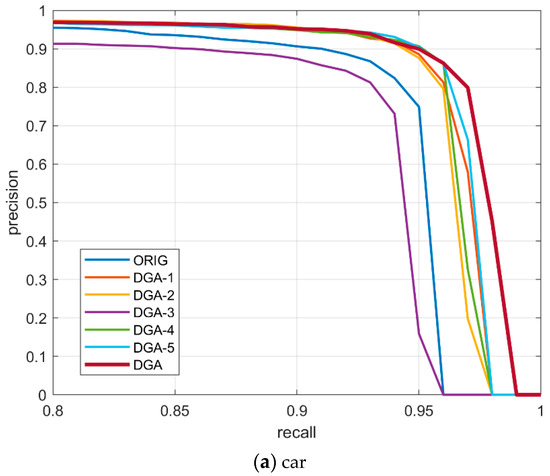
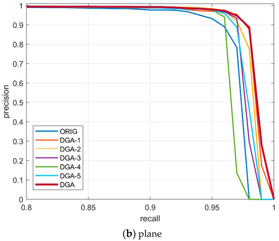
Figure 5.
Precision-recall curves of different classification networks used on the UCAS-AOD dataset.
Some qualitative results between the original network and our proposed DGA module are illustrated in Figure 6. Both models can realize the detection of car and plane objects in complex backgrounds. However, there are some differences between these two networks. On the one hand, the prediction confidence of the propose model for significant objects is higher. On the other hand, there were more mispredictions and omissions for the original network. Some car objects in the shadow could not be predicted accurately. Compared with the original network, the proposed method could better overcome the interference of similar objects in the background.
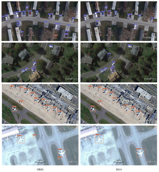
Figure 6.
Selected detection results of the original network and the DGA network. The first column shows the results of the original network, while the second column shows the results of DGA.
4.2.2. Evaluation of United Bounding Regression
The original bounding box regression directly estimate the center point offset coordinating with height and width, which treats these points as independent variables. However, this method ignores the integrity of the bounding box itself. In order to improve the convergence speed and accuracy of regression, united bounding regression based on IoU was adopted instead of the original independent regression of size and offset. Focal Loss was selected as the classification module, which is same as the original network. At the same time, IoU, DioU, and CIoU were adopted for the regression of borders to qualitative analyze the influence of the bounding box regression on the prediction network.
In Table 2 it can be seen that the prediction network reached the best performance when CIoU was adopted. This is because CioU loss simultaneously considers the overlapping area, the distance between center points, and the aspect ratio. From the data, we can see that the mAP improved from 0.942 (ORIG) to 0.964 (CIOU) and mRecall improved from 0.968 to 0.985.
Table 2.
Performance comparison among different settings of regression module. UBR, united bounding regression; AP, average precision.
4.2.3. Evaluation of Combining DGA and UBR
The proposed DGANet network combines DGA with the UBR module to improve detector performance in remote sensing images. The comparison results are listed in Table 3.
Table 3.
Performance of combining DGA and UBR.
Compared with a single module improvement, the DGANet network performance is more advantageous. The mean average precision rose further to 0.971 and the mean recall reached 0.987. Compared with the original network, the accuracy increased by 2.9% and the mRecall increased by 1.9%. We improved the Centernet with a dynamic gradient adjustment mechanism, since it significantly increased the ability of the network to learn effective features and almost no reduction of the network operation speed. DGANet achieved a better convergence speed compared with the original network.
4.2.4. Evaluation of Backbone Model
Table 4 compares the performance of the updated anchor-free detector based on different backbones: ResNet101, Hourglass, and DLA34, and the effect of the deformable convolution layer was also experimentally compared. From the table, it can be seen that the performance of Hourglass or DLA34 is obviously better than that of ResNet101. The mAP of ResNet101 can reach 0.891, which decreases about six percentage points compared with either of the other two backbones. We added the DCN block over the ResNet101 and DLA34, since it adaptively adjusts according to the scale and shape of the objects. This module resulted in a promotion of 1.9% and 1% on mAP for the ReseNet101 and DLA34, respectively. P-R curves of different backbone models are shown in Figure 7, our studies demonstrate that the DLA34 combined with DCN is considerably better compared with other backbone models.
Table 4.
Evaluation results of different backbone models used on the UCAS-AOD dataset.
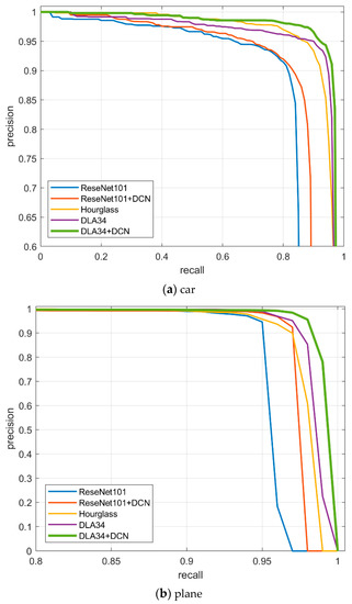
Figure 7.
Precision-recall curves of different backbone models used on the UCAS-AOD dataset.
4.3. Comparison with the State-of-the-Art Methods
We compared the proposed DGANet with the state-of-the-art algorithms on two datasets: UCAS-AOD and LEVIR. Experimental results demonstrate that the performance of DGANet exceeds all other published methods.
Results on UCAS-AOD. We performed extensive comparison between the proposed detector with other state-of-the-art methods used on the UCAS-AOD dataset. Among the comparison experiments, we chose some well-known frameworks, such as Faster RCNN, YOLOv2, SSD, RFCN, and YOLOv4. In addition, many deep CNNs such as VGG-Net, ResNet50, ResNet101, GooLeNet, and DenseNet65 were involved. The overall comparison performance is listed in Table 5.
Table 5.
Evaluation results for the UCAS-AOD dataset.
In this section, we mainly compare the average precision among multiple frameworks and baselines. From the table, it can be noticed that our method achieved 0.956 for the average precision of the car and 0.987 for the average precision of the plane, and both results are highly competitive with the existing published methods. The mAP of our proposed method reached 0.971. From the results, we note that the precision of our approach is considerably better than that of other methods. Figure 8 shows typical detection results on UCAS-AOD dataset by the proposed method. It can be seen that DGANet can detect objects accurately in a variety of challenging backgrounds, and it performs well in a densely arranged scene.
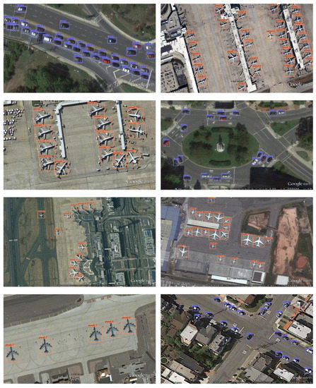
Figure 8.
Detection illustration on the UCAS-AOD dataset.
Results on LEVIR. We compare DGANet predicted results with other models on the LEVIR dataset. LEVIR is a new remote sensing images dataset, which has three categories and is used to realize horizontal bounding box target detection. We also compare our network with other competitive methods, such as Faster RCNN, Sig-NMS, SSD300, RetinaNet500, and Centernet. Table 6 shows the comparison results among different models on the LEVIR dataset. From the data in Table 6 it is apparent that DGANet achievds 0.863 for the mAP, which pulls away from other existing published methods. Compared with the well-known methods Faster RCNN and SSD, DGANet outperformed them with a 6.1% and 7% promotion on mAP.
Table 6.
Evaluation results on the LEVIR dataset.
Compared with the original networks, the proposed detector results in improvements of 1.9%, 4.3%, and 4.4% respectively on AP for the plane, ship, and oil-tank dataset. The mAP is improved from 0.828 to 0.863 with a increasement of 3.5% by using dynamic gradient adjustment mechanism and CioU regression module. Figure 9 shows some detection results on the LEVIR by using the proposed DGANet method.
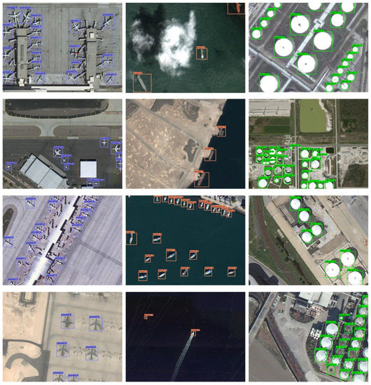
Figure 9.
Detection illustration on the LEVIR dataset.
5. Conclusions
In this article, we proposes a center-point network based on the dynamic gradient adjustment mechanism for object recognition in the remote sensing field. The dynamic gradient adjustment mechanism embedded into the classification loss function is put forward to harmonize the quantity imbalance between easy and hard examples as well as between positive and negative examples. Furthermore, the Complete-IoU loss function is used for the regression of bounding boxes, which converges much more accurately and faster in training. Finally, we describe ablation experiments performed on the UCAS-AOD and LEVIR datasets to evaluate the performance of DGANet. The results demonstrate that the proposed network achieves state-of-the-art prediction accuracy. In the future, we would like to explore the arbitrary-oriented object detection and further improve the model performance in small object detection.
Author Contributions
Conceptualization, P.W.; methodology, P.W.; software, P.W.; validation, C.Z. and Y.N.; formal analysis, P.W. and R.X.; writing—original draft preparation, P.W. and F.M.; writing—review and editing, P.W. and R.X.; visualization, F.M.; supervision, C.Z. and Y.N. All authors have read and agreed to the published version of the manuscript.
Funding
This research received no external funding.
Institutional Review Board Statement
Not applicable.
Informed Consent Statement
Not applicable.
Data Availability Statement
The data used to support the findings of this study are available from the corresponding author upon request.
Conflicts of Interest
The authors declare no conflict of interest.
References
- Cheng, G.; Han, J. A survey on object detection in optical remote sensing images. ISPRS J. Photogramm. Remote Sens. 2016, 117, 11–28. [Google Scholar] [CrossRef]
- Alshehhi, R.; Marpu, P.R.; Woon, W.L.; Mura, M.D. Simultaneous extraction of roads and buildings in remote sensing imagery with convolutional neural networks. ISPRS J. Photogramm. Remote Sens. 2017, 130, 139–149. [Google Scholar] [CrossRef]
- Ding, J.; Xue, N.; Long, Y.; Xia, G.S.; Lu, Q. Learning roi transformer for orientedobject detection in aerial images. In Proceedings of the 2019 IEEE/CVF Conference on Computer Vision and Pattern Recognition (CVPR), Long Beach, CA, USA, 15–20 June 2019; pp. 2849–2858. [Google Scholar]
- Hossain, D.M.; Chen, D.M. Segmentation for Object-Based Image Analysis (OBIA): A review of algorithms and challenges from remote sensing perspective. ISPRS J. Photogramm. Remote Sens. 2019, 150, 115–134. [Google Scholar] [CrossRef]
- Xia, G.S.; Bai, X.; Ding, J.; Zhu, Z.; Belongie, S.; Luo, J.B.; Datcu, M.; Pelillo, M.; Hang, L.P. DOTA: A Large-scale Dataset for Ob-ject Detection in Aerial Images. In Proceedings of the 2018 IEEE/CVF Conference on Computer Vision and Pattern Recognition, Salt Lake City, UT, USA, 18–23 June 2018; pp. 3974–3983. [Google Scholar]
- Guo, Y.; Liu, Y.; Oerlemans, A.; Lao, S.; Wu, S.; Lew, M.S. Deep learning for visual understanding: A review. Neurocomputing 2016, 187, 27–48. [Google Scholar] [CrossRef]
- Girshick, R.; Donahue, J.; Darrell, T.; Malik, J. Region-based convolutional networks for accurate object detection and segmentation. IEEE Trans. Pattern Anal. 2016, 38, 142–158. [Google Scholar] [CrossRef]
- He, K.; Zhang, X.; Ren, S.; Sun, J. Spatial pyramid pooling in deep convolutional networks for visual recognition. IEEE Trans. Pattern Anal. 2015, 37, 1904–1916. [Google Scholar] [CrossRef] [PubMed]
- Girshick, R. Fast R-CNN. In Proceedings of the 2015 IEEE International Conference on Computer Vision (ICCV), Santiago, Chile, 7–13 December 2015; pp. 1440–1448. [Google Scholar]
- Girshick., R.; Donahue, J.; Darrell, T.; Malik, J. Rich feature hierarchies for accurate object detection and semantic segmentation. In Proceedings of the 2014 IEEE Conference on Computer Vision and Pattern Recognition (CVPR), Columbus, OH, USA, 24–27 June 2014; pp. 580–587. [Google Scholar]
- Dai, J.; Li, Y.; He, K.; Sun, J. R-FCN: Object detection via region based fully convolutional networks. In Proceedings of the 30th International Conference on Neural Information Processing Systems, Barelona, Spain, 5–10 December 2016; pp. 379–387. [Google Scholar]
- He, K.; Gkioxari, G.; Dollar, P.; Girshick, R. Mask RCNN. In Proceedings of the 2017 IEEE International Conference on Computer Vision (ICCV), Venice, Italy, 22–29 October 2017; pp. 2980–2988. [Google Scholar]
- Uijlings, J.R.R.; Van De Sande, K.E.A.; Gevers, T.; Smeulders, A.W.M. Selective search for object recognition. Int. J. Comput. Vis. 2013, 104, 154–171. [Google Scholar] [CrossRef]
- Liu, W.; Anguelov, D.; Erhan, D.; Szegedy, C.; Reed, S.; Fu, C.; Berg, A. SSD: Single shot multibox detector. In Proceedings of the European Conference on Computer Vision (ECCV) (2016), Amsterdam, The Netherlands, 8–16 October 2016; pp. 21–37. [Google Scholar]
- Cao, Z.; Hidalgo Martinez, G.; Simon, T.; Wei, S.-E.; Sheikh, Y.A. OpenPose: Realtime Multi-Person 2D Pose Estimation using Part Affinity Fields. IEEE Trans. Pattern Anal. Mach. Intell. 2019, 1–14, in press. [Google Scholar] [CrossRef]
- Zhang, C.; Pan, X.; Li, H.; Gardiner, A.; Sargent, I.; Hare, J.; Atkinson, P.M. A hybrid MLP-CNN classifier for very fine resolution remotely sensed image classification. ISPRS J. Photogramm. Remote Sens. 2017, 140, 133–144. [Google Scholar] [CrossRef]
- Paoletti, M.E.; Haut, J.M.; Plaza, J.; Plaza, A. A new deep convolutional neural network for fast hyperspectral image classifi-cation. ISPRS J. Photogramm. Remote Sens. 2017, 145, 120–147. [Google Scholar] [CrossRef]
- Cui, Z.; Xiao, S.; Feng, J.; Yan, S. Recurrently Target-Attending Tracking. In Proceedings of the 2016 IEEE Conference on Computer Vision and Pattern Recognition (CVPR), Las Vegas, NV, USA, 27–30 June 2016; pp. 1449–1458. [Google Scholar]
- Cheng, G.; Zhou, P.; Han, J. Learning Rotation-Invariant Convolutional Neural Networks for Object Detection in VHR Optical Remote Sensing Images. IEEE Trans. Geosci. Remote Sens. 2016, 54, 7405–7415. [Google Scholar] [CrossRef]
- Li, K.; Cheng, G.; Bu, S.; You, X. Rotation-insensitive and context-augmented object detection in remote sensing images. IEEE Trans. Geosci. Remote Sens. 2017, 2337–2348. [Google Scholar] [CrossRef]
- Deng, Z.; Sun, H.; Zhou, S.; Zhao, J.; Lei, L.; Zou, H. Multi-scale object detection in remote sensing imagery with convolutional neural networks. ISPRS J. Photogramm. Remote Sens. 2018, 145, 3–22. [Google Scholar] [CrossRef]
- Yu, Y.; Gu, T.; Guan, H.; Li, D.; Jin, S. Vehicle Detection from High-Resolution Remote Sensing Imagery Using Convolutional Capsule Networks. IEEE Geosci. Remote Sens. Lett. 2019, 16, 1894–1898. [Google Scholar] [CrossRef]
- Algamdi, A.M.; Sanchez, V.; Li, C.T. Dronecaps: Recognition of Human Actions in Drone Videos Using Capsule Networks with Binary Volume Comparisons. In Proceedings of the 2020 IEEE International Conference on Image Processing (ICIP), Abu Dhabi, United Arab Emirates, 25–28 October 2020. [Google Scholar]
- Mekhalfi, M.L.; Bejiga, M.B.; Soresina, D.; Melgani, F.; Demir, B. Capsule networks for object detection in UAV imagery. Remote Sens. 2021, 11, 1694. [Google Scholar] [CrossRef]
- Chen, Z.; Zhang, J.; Tao, D. Recursive Context Routing for Object Detection. Int. J. Comput. Vis. 2021, 129, 142–160. [Google Scholar] [CrossRef]
- Yu, Y.; Gao, J.; Liu, C.; Guan, H.; Li, D.; Yu, C.; Jin, S.; Li, F.; Li, J. OA-CapsNet: A One-Stage Anchor-Free Capsule Network for Geospatial Object Detection from Remote Sensing Imagery. Can. J. Remote Sens. 2021, 6, 1–4. [Google Scholar] [CrossRef]
- Ren, S.; He, K.; Girshick, R.; Sun, J. Faster R-CNN: Towards real time object detection with region proposal networks. IEEE Trans. Pattern Anal. 2017, 39, 1137–1149. [Google Scholar] [CrossRef]
- Redmon, J.; Farhad, A. YOLO9000: Better, faster, stronger. In Proceedings of the 2017 IEEE Conference on Computer Vision and Pattern Recognition (CVPR), Honolulu, HI, USA, 21–26 July 2017; pp. 6517–6525. [Google Scholar]
- Redmon, J.; Farhadi, A. YOLOv3: An Incremental Improvement. arXiv 2018, arXiv:1804.02767. [Google Scholar]
- Lin, T.-Y.; Goyal, P.; Girshick, R.B.; He, K.; Dollar, P. Focal Loss for Dense Object Detection. IEEE Trans. Pattern Anal. Mach. Intell. 2020, 42, 318–327. [Google Scholar] [CrossRef]
- Lin, T.-Y.; Dollar, P.; Girshick, R.; He, K.; Hariharan, B.; Belongie, S. Feature Pyramid Networks for Object Detection. In Proceedings of the 2017 IEEE Conference on Computer Vision and Pattern Recognition (CVPR), Honolulu, HI, USA, 21–26 July 2017; pp. 936–944. [Google Scholar]
- Law, H.; Deng, J. CornerNet: Detecting Objects as Paired Keypoints. In Proceedings of the Advances in Information Retrieval; Springer: Berlin/Heidelberg, Germany, 2018; pp. 765–781. [Google Scholar]
- Law, H.; Teng, Y.; Russakovsky, Y.; Deng, J. Cornernetlite: Efficient keypoint based object detection. arXiv 2019, arXiv:1904.08900. [Google Scholar]
- Rashwan, A.; Agarwal, R.; Kalra, A.; Poupart, P. Matrix Nets: A New Scale and Aspect Ratio Aware Architecture for Object Detection. In Proceedings of the 2019 IEEE/CVF International Conference on Computer Vision Workshop (ICCVW), Seoul, Korea, 27–28 October 2019; pp. 2025–2028. [Google Scholar]
- Duan, K.; Bai, S.; Xie, L.; Qi, H.; Huang, Q.; Tian, Q. CenterNet: Keypoint Triplets for Object Detection. In Proceedings of the 2019 IEEE/CVF International Conference on Computer Vision (ICCV), Seoul, Korea, 27–28 October 2019; pp. 6568–6577. [Google Scholar]
- Zhou, X.; Wang, D.; Krahenbuhl, P. Objects as points. arXiv 2019, arXiv:1904.07850. [Google Scholar]
- Li, B.; Liu, Y.; Wang, X. Gradient Harmonized Single-Stage Detector. In Proceedings of the AAAI Conference on Artificial Intelligence; Association for the Advancement of Artificial Intelligence (AAAI): Menlo Park, CA, USA, 2019; Volume 33, pp. 8577–8584. [Google Scholar]
- Yu, F.; Wang, D.; Shelhamer, E.; Darrell, T. Deep Layer Aggregation. In Proceedings of the 2018 IEEE/CVF Conference on Computer Vision and Pattern Recognition, Salt Lake City, UT, USA, 18–23 June 2018; pp. 2403–2412. [Google Scholar]
- Dai, J.; Qi, H.; Xiong, Y.; Li, Y.; Zhang, G.; Hu, H.; Wei, Y. Deformable convolutional networks. In Proceedings of the 2017 IEEE International Conference on Computer Vision (ICCV), Venice, Italy, 22 October 2017; pp. 764–773. [Google Scholar]
- Zheng, Z.H.; Wang, P.; Liu, W.; Li, J.Z.; Ye, R.G.; Ren, D.W. Distance-IoU Loss: Faster and Better Learning for Bounding Box Regression. In Proceedings of the AAAI Conference on Artificial Intelligence; Association for the Advancement of Artificial Intelligence (AAAI): Menlo Park, CA, USA, 2020; Volume 34, pp. 12993–13000. [Google Scholar]
- Chen, X.; Xiang, S.; Liu, C.-L.; Pan, C.-H. Vehicle Detection in Satellite Images by Hybrid Deep Convolutional Neural Networks. IEEE Geosci. Remote Sens. Lett. 2014, 11, 1797–1801. [Google Scholar] [CrossRef]
- Zou, Z.; Shi, Z. Ship Detection in Spaceborne Optical Image with SVD Networks. IEEE Trans. Geosci. Remote Sens. 2016, 54, 5832–5845. [Google Scholar] [CrossRef]
- Han, X.; Zhong, Y.; Zhang, L. An Efficient and Robust Integrated Geospatial Object Detection Framework for High Spatial Resolution Remote Sensing Imagery. Remote Sens. 2017, 9, 666. [Google Scholar] [CrossRef]
- Ding, P.; Zhang, Y.; Deng, W.J.; Jia, P.; Kuijper, A. A light and faster regional convolutional neural network for object detection in optical remote sensing images. ISPRS J. Photogramm. Remote Sens. 2018, 141, 208–218. [Google Scholar] [CrossRef]
- Shrivastava, A.; Gupta, A.; Girshick, R. Training Region-Based Object Detectors with Online Hard Example Mining. In Proceedings of the 2016 IEEE Conference on Computer Vision and Pattern Recognition (CVPR), Las Vegas, NV, USA, 26 June–1 July 2016; pp. 761–769. [Google Scholar]
- Ying, X.; Wang, Q.; Li, X.W.; Yu, M.; Yu, R.G. Multi-attention object detection model in remote sensing images based on multi-scale. IEEE Access 2019, 7, 94508–94519. [Google Scholar] [CrossRef]
- Zhou, X.; Zhuo, J.; Krahenbuhl, P. Bottom-Up Object Detection by Grouping Extreme and Center Points. In Proceedings of the 2019 IEEE/CVF Conference on Computer Vision and Pattern Recognition (CVPR), Long Beach, CA, USA, 15–20 June 2019; pp. 850–859. [Google Scholar]
- Zhu, H.Q.; Chen, X.; Dai, W.; Fu, K.; Ye, Q.; Jiao, J. Orientation robust object detection in aerial images using deep convolutional neural network. In Proceedings of the 2015 IEEE International Conference on Image Processing (ICIP), Quebec City, QC, Canada, 27–30 September 2015; pp. 3735–3739. [Google Scholar]
- Zou, Z.X.; Shi, Z.W. Random access memories: A new paradigm for target detection in high resolution aerial remote sensing images. IEEE Trans. Image Process. 2018, 27, 1100–1111. [Google Scholar] [CrossRef]
- Fu, K.; Chang, Z.; Zhang, Y.; Xu, G.; Zhang, K.; Sun, X. Rotation-aware and multi-scale convolutional neural network for object detection in remote sensing images. ISPRS J. Photogramm. Remote Sens. 2020, 161, 294–308. [Google Scholar] [CrossRef]
- Yang, X.; Sun, H.; Fu, K.; Yang, J.; Sun, X.; Yan, M.; Guo, Z. Automatic Ship Detection in Remote Sensing Images from Google Earth of Complex Scenes Based on Multiscale Rotation Dense Feature Pyramid Networks. Remote Sens. 2018, 10, 132. [Google Scholar] [CrossRef]
- Bochkovskiy, A.; Wang, C.Y.; Liao, H.Y. YOLOv4: Optimal Speed and Accuracy of Object Detection. arXiv 2020, arXiv:2004.10934. [Google Scholar]
- Bao, S.; Zhong, X.; Zhu, R.; Zhang, X.; Li, Z.; Li, M. Single Shot Anchor Refinement Network for Oriented Object Detection in Optical Remote Sensing Imagery. IEEE Access 2019, 7, 87150–87161. [Google Scholar] [CrossRef]
- Yang, X.; Yang, J.; Yan, J.; Zhang, Y.; Zhang, T.; Guo, Z.; Sun, X.; Fu, K. SCRDet: Towards More Robust Detection for Small, Cluttered and Rotated Objects. In Proceedings of the 2019 IEEE/CVF International Conference on Computer Vision (ICCV), Seoul, Korea, 27 October–2 November 2019; pp. 8231–8240. [Google Scholar]
- Wang, Y.Y.; Li, H.F.; Jia, P.; Zhang, G.; Wang, T.; Hao, X. Multi-scale densenets-based aircraft detection from remote sensing images. Sensors 2019, 19, 5270. [Google Scholar] [CrossRef]
- Li, C.; Xu, C.; Cui, Z.; Wang, D.; Zhang, T.; Yang, J. Feature-Attentioned Object Detection in Remote Sensing Imagery. In Proceedings of the 2019 IEEE International Conference on Image Processing (ICIP), Taipei, Taiwan, 22–25 September 2019; pp. 3886–3890. [Google Scholar]
- Dong, R.; Xu, D.; Zhao, J.; Jiao, L.; An, J. Sig-NMS-Based Faster R-CNN Combining Transfer Learning for Small Target Detection in VHR Optical Remote Sensing Imagery. IEEE Trans. Geosci. Remote Sens. 2019, 57, 8534–8545. [Google Scholar] [CrossRef]


Publisher’s Note: MDPI stays neutral with regard to jurisdictional claims in published maps and institutional affiliations. |
© 2021 by the authors. Licensee MDPI, Basel, Switzerland. This article is an open access article distributed under the terms and conditions of the Creative Commons Attribution (CC BY) license (https://creativecommons.org/licenses/by/4.0/).