Using Multi-Angular Hyperspectral Data to Estimate the Vertical Distribution of Leaf Chlorophyll Content in Wheat

Abstract

Heterogeneity exists in the vertical distribution of the biochemical components of crops. A leaf chlorophyll deficiency occurs in the bottom- and middle-layers of crops due to nitrogen stress and leaf senescence. Some studies used multi-angular remote sensing data for estimating the vertical distribution of the leaf chlorophyll content (LCC). However, these studies performed LCC inversion of different vertical layers using a fixed view zenith angle (VZA), but rarely considered the contribution of the components of the non-target layers to the spectral response. The main goal of this work was to determine the LCC of different vertical layers of the canopy of winter wheat (Triticum aestivum L.), using multi-angular remote sensing and spectral vegetation indices. Different combinations of VZAs were used for obtaining the LCC of different layers. The results revealed that the responses of the transformed chlorophyll in reflectance absorption index (TCARI) and modified chlorophyll absorption in reflectance index (MCARI)/optimized soil-adjusted vegetation index (OSAVI) to the upper-layer LCC were strongest at VZA 10°. For the middle-layer LCC, the response was strongest at 30°, but the response was significantly lower than that of the upper-layer. For the bottom-layer LCC, the responses were weak due to the obscuring effect of the upper- and middle-layer; thus, the LCC inversion of the bottom-layer data was not optimal for a single VZA. The optimal VZA or VZA combinations for LCC estimation were VZA 10° for the upper-layer LCC (TCARI with coefficient of determination (R²) = 0.69, root mean square error (RMSE) = 4.80 ug/cm², MCARI/OSAVI with R² = 0.73, RMSE = 4.17 ug/cm²), VZA 10° and 30° for the middle-layer LCC (TCARI with R² = 0.17, RMSE = 4.81 ug/cm², MCARI/OSAVI with R² = 0.17, RMSE = 4.76 ug/cm²), and VZA 10°, 30°, and 50° for the bottom-layer LCC (TCARI with R² = 0.40, RMSE = 6.29 ug/cm², MCARI/OSAVI with R² = 0.40, RMSE = 6.36 ug/cm²). The proposed observation strategy provided a significantly higher estimation accuracy of the target layer LCC than the single VZA approach, and demonstrated the ability of canopy multi-angular spectral reflectance to accurately estimate the wheat canopy chlorophyll content vertical distribution.

1. Introduction

The importance of analyzing the leaf chlorophyll content (LCC) in vegetation has been recognized for decades [1,2,3,4]. The LCC depends on the photosynthetic capacity, developmental stage, and canopy stress [5,6,7]. It has been suggested that the LCC can be used to predict crop yield [8].

Nitrogen (N) exhibits a pronounced heterogeneity in the vertical distribution in crop canopies since it is highly mobile [9,10]. If the N demand of a crop is higher than its uptake, N is efficiently translocated to the photosynthetically most active leaves in the top canopy [11]. Therefore, N deficiency generally occurs in the lower layer leaves. Nitrogen is an important substance for chlorophyll synthesis. The deficiency of nitrogen is accompanied by the decrease of chlorophyll content, which is manifested as leaf wither and yellow. Timely and accurate monitoring of chlorophyll content can effectively obtain the growth status of crops. Remote sensing provides an alternative to large-area LCC analysis of crops. Various methods have been presented for estimating the canopy chlorophyll content using hyperspectral reflectance data. However, the vertical chlorophyll gradient is not considered in most top-of-the-canopy remote sensing techniques. The use of multiple viewing angles may improve the detection of the canopy architecture, leaf area index (LAI), and leaf chemical parameters of the canopy overstory and understory vegetation since differences in light scattering and shadowing depend on the vegetation layer and the phenology of the understory vegetation [12,13,14]. Methods for estimating crop chlorophyll content using hyperspectral resolution remote sensing data can be divided into the following three categories: chlorophyll content monitoring based on light reflection and its derivative, logarithm, etc. [15,16,17,18], chlorophyll content monitoring based on red edge parameters and chlorophyll content monitoring based on physical models. From a mathematical point of view, vegetation index is also a spectral derived parameter, but due to the absorption characteristics of chlorophyll, water, and dry matter in vegetation, it has formed its unique spectral characteristics, and has been widely used in the research of crop chlorophyll remote sensing monitoring [19,20,21]. Vegetation indices exhibit directionality effects because of the canopy structure, canopy composition, background, shadowing [22,23], as well as the sensor view angle. Vegetation indices based on multiple view zenith angles (VZAs) have the potential to improve the estimation of the vertical distribution of the LCC in the crop canopy [12,24,25,26].

The winter wheat (Triticum aestivum L.) canopy can be regarded as consisting of different layers. Substantial differences exist in the reflection and scattering of electromagnetic waves in different canopy layers due to different light conditions of the leaves. Leaves in different layers have different contributions to the canopy hyperspectral reflectance, affecting the remote sensing assessments of the crop’s biochemical properties (e.g., LCC) [27]. It is crucial to define the contribution of the leaves in different layers to the canopy’s spectral reflectance to increase the accuracy of estimating the vertical distribution of the LCC. At a given VZA, the spectrum contains LCC information from different layers. The contribution of the LCC from other layers and the influences on the layer of interest should also be considered to determine the LCC of the crop in different layers. In recent years, monitoring of the vertical distribution of different components of the crop canopy [28,29,30,31,32,33] and different crop varieties [28,29,30,32,33] has received increasing attention. Kong et al. discussed the monitoring ability of two-band and three-band combinations in normalized difference vegetation index (NDVI)-, simple ratio (SR)-, and chlorophyll index(CI)-like types of indices at different viewing angles to LCC vertical distribution [26]. Huang et al. carried out monitoring of LCC vertical distribution by using two VZAs combination [12]. However, until recently, few studies have considered the vertical distribution of the LCC and the contribution to the multi-angular spectrum, and formulate specific monitoring strategies according to the differences in the monitoring difficulty of LCC at different vertical layers. This monitoring strategy would significantly improve the accuracy and practicability of LCC vertical distribution monitoring.

The purpose of this study is to determine the effect of the vertical chlorophyll distribution on the multi-angular spectrum and improve the monitoring ability of the LCC in specific layers. We analyze the contribution of the LCC in different layers to the spectral index at different VZAs to select the optimum VZA or VZA combination for the target layer and improve the monitoring ability of the LCC of the crop in a specific vertical location.

2. Materials and Methods

2.1. Experimental Site and Design

Field experiments were conducted in 2005 and 2007 at the National Experiment Station for Precision Agriculture (40°10.6′N, 116°26.3′E), Beijing, China. The cropping system is winter wheat with summer maize rotation, the most popular system in North China. The field site is located in a warm temperate climate zone in a semi-moist continental monsoon region. The annual average temperature of the experimental site is 10–12 °C, the annual average precipitation is 600–700 mm, and the annual average sunshine time is 2700–2800 h. The seasonal distribution of precipitation is uneven, with 70% occurring from July to September. The field experiments consisted of eleven erect-type wheat varieties, including Jing411, Nongda3291, 9158, Jingdong12, Laizhou3279, I-93, 6211, Jing9843, Lumai21, P7, and Xiaoyan54. The treatment plot size was 45 m × 10.8 m. In the experiment, 345 kg of compound fertilizer (15% N, 15% P, 15% K) and 75 kg of urea were applied per hectare. The spectral and leaf chlorophyll measurements were performed in the typical winter wheat growth stages: 17 April (stem elongation, Z31), 28 April (stem elongation, Z39), 9 May (booting, Z47), 19 May (heading, Z59), and 29 May (Milk-filling, Z73) in 2007. The experimental growth stage in 2005 was matched with that in 2007.

2.2. Data Acquisition

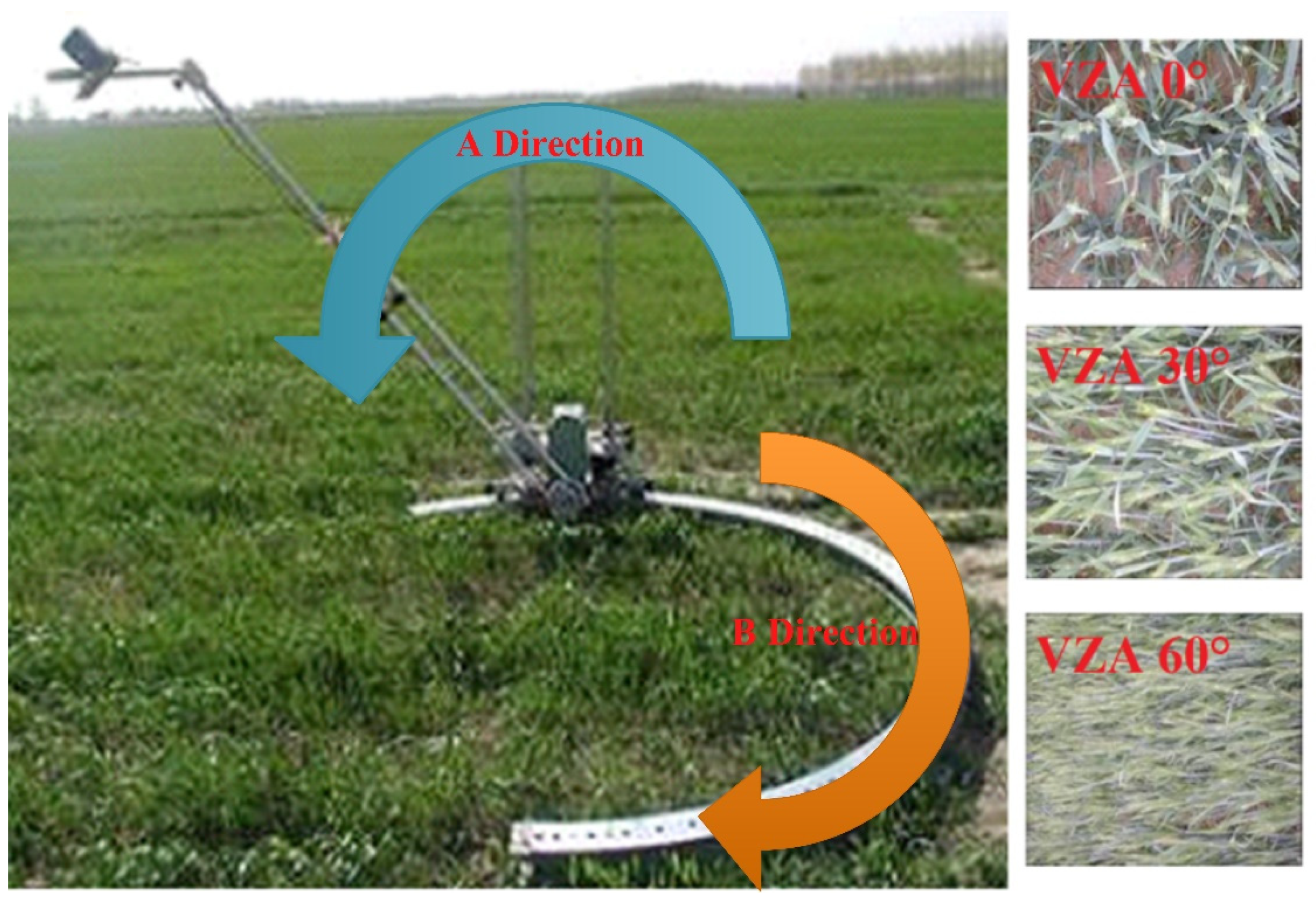
A 1 m² area of the crop canopy was selected in each plot to measure the canopy reflectance under clear sky conditions at 11:00–13:00 local time using an ASD FieldSpec 3 spectrometer (Analytical Spectral Devices, Boulder, CO, USA) fitted with a 25°-field-of-view fiber optic adaptor. Each spectral measurement was preceded by a dark current measurement, and a white reference measurement was taken using a white Spectralon (Labsphere, Inc., North Sutton, NH, USA) reference panel. The sensor was placed at the height of 1 m above the canopy on top of the zenith arc of a goniometer. The observation azimuth was relatively fixed as the sun direction, as seen from the observation point. The VZA ranged from 0° to +60° at intervals of 10° in each plot (expect for VZA 5°), and ten scans were averaged into a single spectral sample (Figure 1). The multi-angular observation device has 3 moving parts to adjust the observation position and direction. The adjustment in A direction is to change the VZA, the direction of observation plane can be adjusted in B direction, and the length of the swing arm can also be adjusted to change the sensor receiving distance to the canopy.

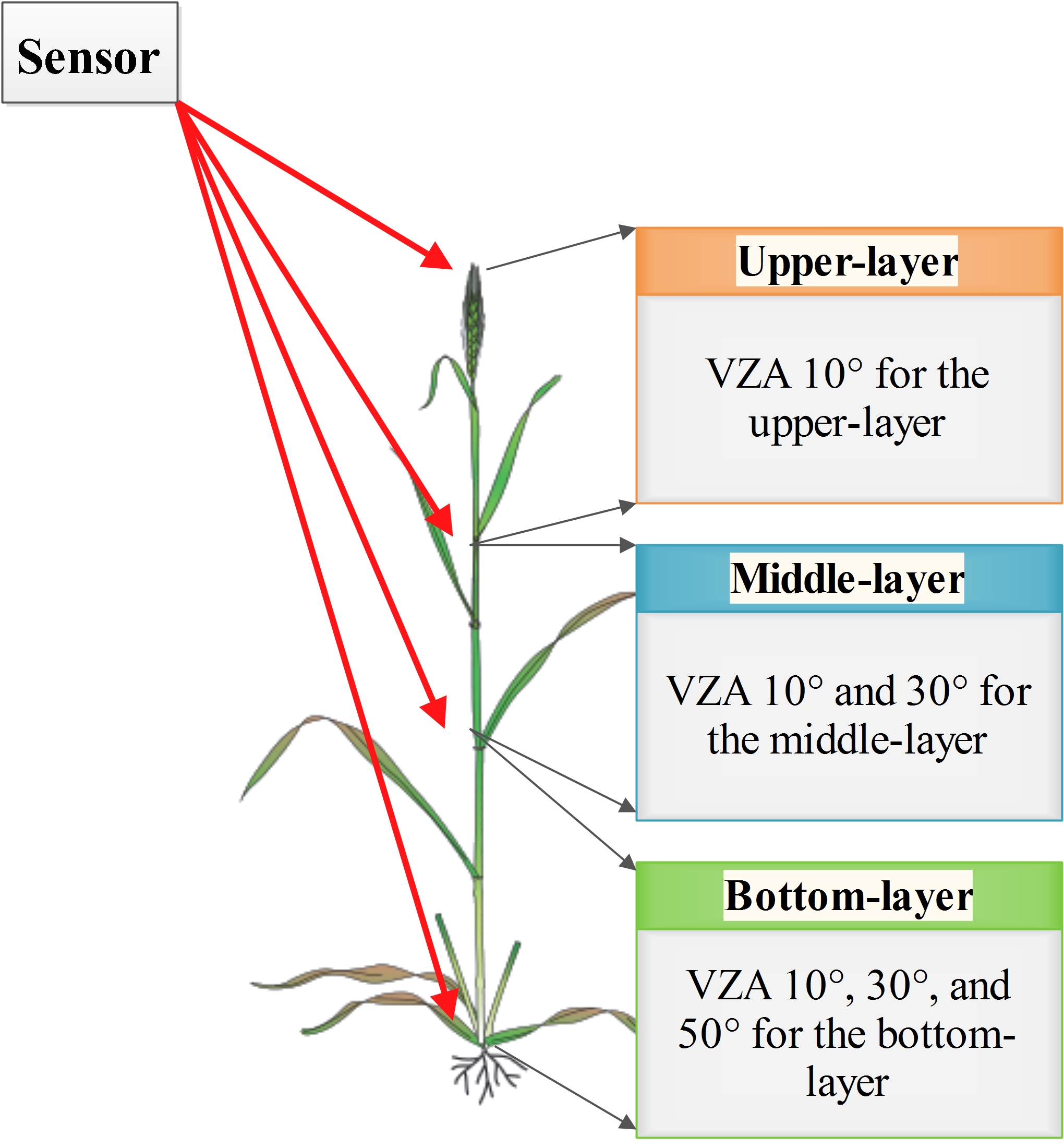
In order to simplify the study, wheat canopy leaves at different growth stages were vertically stratified. The stratification method in the previous studies, to some extent, referred to the agronomic stratification method of wheat [26]. There was a problem that the vertical depth (distance from the top of the canopy) of a particular layer changes at different growth stages. In order to meet the needs of remote sensing monitoring research, the distance of different layers to the top of the canopy was taken as the basis of stratification. Plant leaves were cut off and divided into two or three layers, according to their positions in the canopy. The top 1st and 2nd leaves were assigned to the upper-layer, the top 3rd leaves were assigned to the middle-layer, and the top 4th and the leaves below were assigned to the bottom-layer. Leaves sampled at the stem-elongation stage were divided only into the upper- and middle-layers due to the limited number of leaves in that stage.

The leaf fresh weight (FW) of the sample (0.5 g) was obtained by 80% acetone extraction. The visible light absorption spectrum of the pigments was determined with the spectrophotometer at 663 nm and 645 nm. We used the following equation to calculate the chlorophyll a and chlorophyll b contents.

$${\mathrm{Chl}}_{\mathrm{a}}\left(\mathrm{mg}/\mathrm{g}\right)=\left[\left(12.25{\mathrm{A}}_{663}-2.79{\mathrm{A}}_{645}\right)\times {\mathrm{V}}_{\mathrm{T}}\left(\mathrm{mL}\right)]/[\mathrm{DW}\left(\mathrm{g}\right)\times 1000\right]$$

(1)

$${\mathrm{Chl}}_{\mathrm{b}}\left(\mathrm{mg}/\mathrm{g}\right)=\left[\left(21.50{\mathrm{A}}_{645}-5.10{\mathrm{A}}_{663}\right)\times {\mathrm{V}}_{\mathrm{T}}\left(\mathrm{mL}\right)]/[\mathrm{DW}\left(\mathrm{g}\right)\times 1000\right]$$

(2)

where Chl_a and Chl_b refer to the concentrations of chlorophyll a and b. A₆₆₃ and A₆₄₅ are the absorption spectra of the pigments extracted at 663 nm and 645 nm, respectively. According to the volume of the pigment extract (V_T), the dry weight (DW), and area of the leaves (LA), the unit of the pigment content can be converted to the concentration and the pigment content per unit leaf area (ug/cm²). The conversion formula is as follows:

$${\mathrm{Chl}}_{\mathrm{a}+\mathrm{b}}\left(\mathsf{\mu }\mathrm{g}/{\mathrm{cm}}^2\right)=\left[\left({\mathrm{Chl}}_{\mathrm{a}}\left(\mathrm{mg}/\mathrm{g}\right)+{\mathrm{Chl}}_{\mathrm{b}}\left(\mathrm{mg}/\mathrm{g}\right)\right)\times \mathrm{DW}\left(\mathrm{g}\right)\times 1000\right]/\mathrm{LA}\left({\mathrm{cm}}^2\right)$$

(3)

where Chl_a+b refer to the concentrations of chlorophyll ab. where LA (cm²) is the leaf area of the sample.

2.3. Chlorophyll-Sensitive Spectral Index Selection

This study makes full use of previous research results and incorporates multiple spectral indices. The chlorophyll absorption in reflectance index (CARI) is a common vegetation index for detecting chlorophyll [34]. Subsequently, the modified chlorophyll absorption in reflectance index (MCARI) and the transformed chlorophyll in reflectance absorption index (TCARI) were proposed (

Table 1. Spectral vegetation indices used in this study.

Index	Formula	Reference
TCARI	3[(R700 − R670) − 0.2(R700 − R550) × (R700/R670)]	[35]
MCARI/OSAVI	[(1 + 0.16) × (R800 − R680)/(R800 + R680 + 0.16)]/[(1 + 0.5) × (R800 − R670)/(R800 + R670 + 0.5)]	[6]

) [35,36].

The CARI uses the 670 nm, 550 nm, and 700 nm bands. Kim believes that the 670 nm band is the strongest absorption band for chlorophyll a, and the 550 nm and 700 nm bands are the strong response band of chlorophyll a [29]. The CARI reduces the effects of changes in photosynthetically active radiation caused by non-photosynthetic materials in the canopy but is substantially affected by the background soil reflectance. It is also difficult to estimate the chlorophyll content at a low LAI. Daughtry stated that a change in the background reflectance affects the first derivative of the reflectance at wavelengths from 550 to 700 nm [35]. The ratio of the reflectance at 700 nm to the reflectance at 670 nm was used to offset this effect, resulting in the TCARI. In addition, we use the MCARI/optimized soil-adjusted vegetation index (OSAVI) to eliminate the influence of background soil reflectance and compare it with the TCARI for determining the LCC.

2.4. Data Analysis

The objectives of this study were to investigate the contribution of the LCC in different layers to the overall spectral response, and select the most suitable VZA and VZA combination to monitor the target layer LCC.

2.4.1. Spectral Influence Analysis Based on Analysis of Variance

The analysis of variance (ANOVA) is one of the basic methods widely used in mathematical statistics. The essence of ANOVA is a hypothesis testing problem to test whether the mean of each population is equal under the assumption of multiple normal population equals variance [36]. The LCC in different vertical layers was taken as a factor, and the variance analysis method was used to explore whether the changes of the state of LCC will lead to the changes of the spectral reflectance indexes, so as to explore their influence on the spectral reflectance. We analyzed the responses of different spectral indices in the different layers, and the effects of the LCC in the non-target layer were minimized by using a combination of VZAs.

2.4.2. Correlation Analysis of Spectral Index and Leaf Chlorophyll Content

Correlation analysis was used to analyze the correlation between the LCC in different vertical layers and the TCARI and MCARI/OSAVI under different VZAs. The results of the correlation analysis provided information on the contribution of the LCC in different layers to the spectral response.

2.4.3. Model Calibration and Validation

Samples in all growth stage were randomly divided into two datasets: Two thirds as the training dataset and one third as the validation dataset. A total of 67 samples were collected in two years; of these 44 were used to build estimation models. Further, 23 samples were used for validation. The interaction effect of the band combinations in the spectral index analysis and the regression analyses was analyzed using a computer program developed in MATLAB 9.0 software (The MathWorks, Inc., Natick, MA, USA) and Excel 2013 (The Microsoft Corporation, Inc., Redmond, WA, USA). The model performance was estimated by comparing the differences in the prediction results using the coefficient of determination (R²) and the root mean square error (RMSE) [26]. The higher the R², and the lower the RMSE, the higher the precision and accuracy of the model are for predicting the LCC.

3. Results

3.1. LCC Distribution in the Wheat Canopy

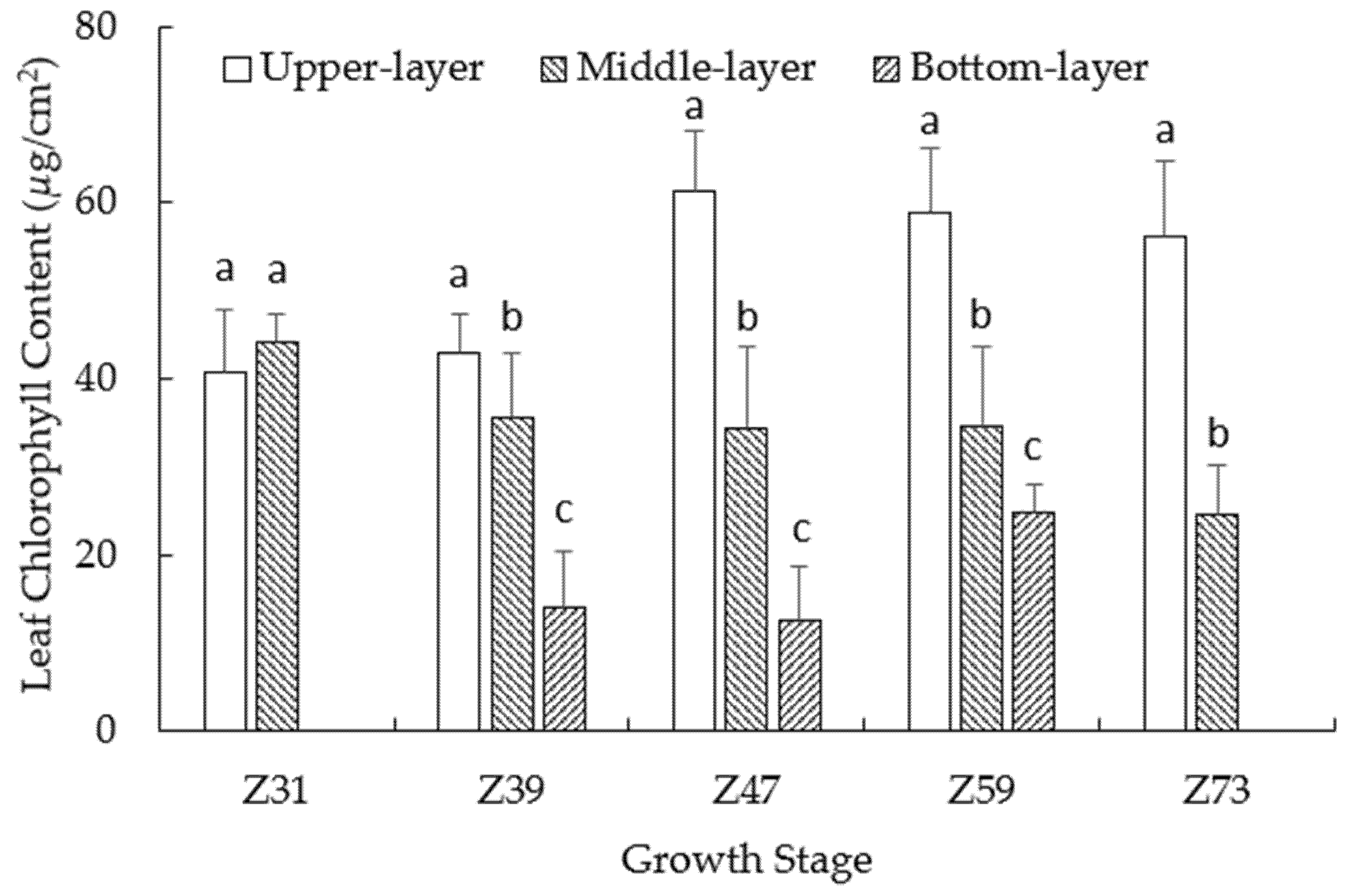
In the jointing stage, the samples had 2 to 3 leaves. According to the canopy layering method used in this study, there were one or two layers of leaves, namely, the upper- and middle-layers. At this growth stage, the shading effect between the leaves was not strong, and the upper-layer LCC was lower than that in the later stage. The LCC of the middle-layer and newer upper-layer were almost identical (Figure 2). In the jointing stage, the wheat was growing fast, and there were three layers of leaves in this stage, but the chlorophyll content had not increased significantly in upper- and middle-layer. The LCC of the lower leaves was lower than that of the upper- and middle-layer leaves. After the booting and heading stages, reproductive development occurred. The LCC of the upper-layer began to increase due to the utilization of light energy, resulting in a significant difference in the chlorophyll content between the upper-, middle-, and bottom-layers. The photosynthetic rate was relatively low in the bottom-layer leaves due to shading and nutrient transfer to the upper-layer leaves.

3.2. View Zenith Angle Selection

Pairwise correlation analysis was performed to determine the correlation between the TCARI or MCARI/OSAVI values at different VZAs (0°, 5°,10°, 20°, 30°, 40°, 50°, and 60°). The more similar the VZAs were, the higher the coefficient of determination was (

Table 2. Coefficient of determination (R²) between the TCARI values at different view zenith angles (VZAs).

	VZA0°		VZA5°		VZA10°		VZA20°		VZA30°		VZA40°		VZA50°		VZA60°
	R2	p Value	R2	p Value	R2	p Value	R2	p Value	R2	p Value	R2	p Value	R2	p Value	R2	p Value
VZA0°	1	-	-	-	-	-	-	-	-	-	-	-	-	-	-	-
VZA5°	0.772	0.000	1	-	-	-	-	-	-	-	-	-	-	-	-	-
VZA10°	0.779	0.000	0.798	0.000	1	-	-	-	-	-	-	-	-	-	-	-
VZA20°	0.721	0.000	0.644	0.000	0.840	0.000	1	-	-	-	-	-	-	-	-	-
VZA30°	0.496	0.010	0.394	0.047	0.603	0.001	0.743	0.000	1	-	-	-	-	-	-	-
VZA40°	0.080	0.696	0.099	0.629	0.007	0.971	0.064	0.757	0.169	0.409	1	-	-	-	-	-
VZA50°	0.193	0.344	0.084	0.683	0.238	0.243	0.140	0.495	0.291	0.149	0.489	0.011	1	-	-	-
VZA60°	0.266	0.188	0.250	0.219	0.378	0.057	0.110	0.591	0.209	0.305	0.471	0.015	0.670	0.000	1	-

and

Table 3. Coefficient of determination (R²) between the MCARI/OSAVI values at different VZAs.

	VZA0°		VZA5°		VZA10°		VZA20°		VZA30°		VZA40°		VZA50°		VZA60°
	R2	p Value	R2	p Value	R2	p Value	R2	p Value	R2	p Value	R2	p Value	R2	p Value	R2	p Value
VZA0°	1	-	-	-	-	-	-	-	-	-	-	-	-	-	-	-
VZA5°	0.783	0.000	1	-	-	-	-	-	-	-	-	-	-	-	-	-
VZA10°	0.805	0.000	0.856	0.000	1	-	-	-	-	-	-	-	-	-	-	-
VZA20°	0.780	0.000	0.795	0.000	0.920	0.000	1	-	-	-	-	-	-	-	-	-
VZA30°	0.696	0.000	0.644	0.000	0.792	0.000	0.861	0.000	1	-	-	-	-	-	-	-
VZA40°	0.276	0.173	0.312	0.121	0.424	0.031	0.482	0.013	0.515	0.007	1	-	-	-	-	-
VZA50°	0.431	0.028	0.323	0.108	0.486	0.012	0.447	0.022	0.572	0.002	0.634	0.001	1	-	-	-
VZA60°	0.487	0.012	0.436	0.026	0.589	0.002	0.460	0.018	0.523	0.006	0.618	0.001	0.778	0.000	1	-

). The difference become prominent when the VZA interval was larger than 20°. Thus, we analyzed the spectral indices at VZAs 10°, 30°, and 50°, at 20° intervals to prevent loss of spectral information to allow for determining the contribution of the LCC in different layers to the spectral response.

The coefficient of determination at VZA 10° and 30° were 0.55 and 0.69 for the TCARI and MCARI/OSAVI, respectively. Those at VZA 30° and 50° were 0.35 and 0.56, and those at VZA 10° and 50° were 0.27 and 0.46, respectively. The coefficient of determination increased significantly from VZA different 20° to 10°; thus, these VZAs (VZA 10°, VZA 30°, and VZA 50°) were suitable to determine the contribution of the LCC in the upper-, middle-, and bottoms-layers to the spectral response.

3.3. Response of the Spectral Indices to the LCC in Different Layers

The following conclusions can be drawn from the ANOVA results of the TCARI and MCARI/OSAVI indices (

Table 4. Factor level of the leaf chlorophyll content in different layers.

Layer	LCC Level (ug/cm2)
	Level 1	Level 2	Level 3
Upper-layer	31.76–42.29	42.46–50.50	50.66–58.51
Middle-layer	20.64–39.83	40.13–43.05	43.76–55.36
Bottom-layer	10.21–26.26	26.48–34.09	34.86–46.01

and

Table 5. F statistic of the interaction of different factors.

Layer	TCARI			MCARI/OSAVI
	VZA10°	VZA30°	VZA50°	VZA10°	VZA30°	VZA50°
Upper-layer	0.22	0.71	0.66	2.25	2.04	2.01
Middle-layer	2.67	0.54	0.68	2.15	0.56	0.39
Bottom-layer	0.66	1.19	0.02	0.82	1.46	0.08
U-layer&M-layer *	1.67	0.78	1.16	0.84	0.47	0.46
U-layer&B-layer **	1.10	0.63	1.04	0.71	0.48	0.76
M-layer&B-layer #	1.00	0.21	1.69	0.50	0.08	1.40
U-layer&M-layer&B-layer ##	1.17	0.28	0.66	0.34	0.47	0.55

* U-layer&M-layer is the Upper-layer & Middle-Layer. ** U-layer&B-layer is the Upper-layer & Bottom-layer. ^# M-layer&B-layer is the Middle-layer& Bottom-layer. ^## U-layer&M-layer&B-layer is the Upper-layer & Middle-layer & Bottom-layer.

). The middle- and bottom-layers leaves were shielded by upper-layer leaves, limiting the penetration ability of electromagnetic waves. Therefore, the spectral response of the vegetation indices decreased with increasing depth. As the VZA changed from VZA 10 to 50°, the effect of the LCC in the upper-layer on the spectral index first decreased and then increased. At VZA 10°, the observation angle was near the vertical, and the upper-layer had the strongest spectral effect. The interaction between the LCC of the middle-, bottom-layers, and the LCC of the upper-layer were weak; thus, this VZA was most suitable for the upper-layer LCC inversion. The bottom-layer leaves were more obscured at VZA 10° and 30° than 50°, and the contribution of the upper and middle-layers to the spectral response was higher. Thus, the largest contribution of the middle-layer LCC was at VZA 30°. Although the effect of the upper-layer was strong at VZA 50°. However, the influence of other layers were strong too, and the VZA 50° was not suitable for monitoring the upper-layer LCC.

The effect of the upper-layer LCC on the TCARI was strong at VZA 10°, and the F statistics was 0.22. For the middle-layer, the effect was strongest at 30° and 50°, and the F statistics were 0.54 and 0.39 for TCARI and MCARI/OSAVI, respectively. The degree of influence was significantly larger for the bottom-layer than the upper-layer. The contribution of the bottom-layer LCC was not strong due to the influence of the upper and middle-layers. Thus, it is not recommended to use an inversion of the bottom-layer LCC when a single VZA is used.

3.4. Correlation Analysis between LCC and Vegetation Indices

We analyzed the correlation between the LCC of different layers obtained from the TCARI and MCARI/OSAVI at different VZAs (

Table 6. Coefficient of determination (R²) of the leaf chlorophyll content obtained from the vegetation indices at different VZAs in the upper-, middle-, and bottom-layers.

Layer	VZA10°	VZA30°	VZA50°	VZA10°	VZA30°	VZA50°
	TCARI			MCARI/OSAVI
Upper-layer	0.30	0.21	0.05	0.09	0.04	0.00
Middle-layer	0.21	0.29	0.14	0.04	0.09	0.02
Bottom-layer	0.04	0.00	0.09	0.00	0.00	0.01

). The results described the correlation between the LCC of the target layer and the spectral index obtained at a given VZA, reflecting the contribution of the LCC of different layers to the spectral response. In previous studies, correlation analysis was also used to select the VZA [29,33].

The largest coefficient of determination of the TCARI for the upper-layer LCC (> 0.30) was obtained at VZA 10° within TCARI. This finding was in line with the results of previous studies. Most of the reflectance information in the spectral response comes from the upper- and middle-layer leaves. The coefficient of determination of the middle-layer LCC were also high than that of bottom-layer. The highest R² were obtained at VZA 30°, both within TCARI and MCARI/OSAVI. The coefficient of determination of the TCARI for the bottom-layer showed a decreasing-increasing trend as the VZA increased within TCARI, and the coefficient of determination was significantly lower than that of the upper- and middle-layers. Therefore, for accurate monitoring of the LCC in bottom-layer, it is necessary to include all VZAs (10°, 30°, and 50°) observations. The ranking of the layers regarding the coefficient of determination was upper-layer > middle-layer > lower-layer.

3.5. Modeling and Validation

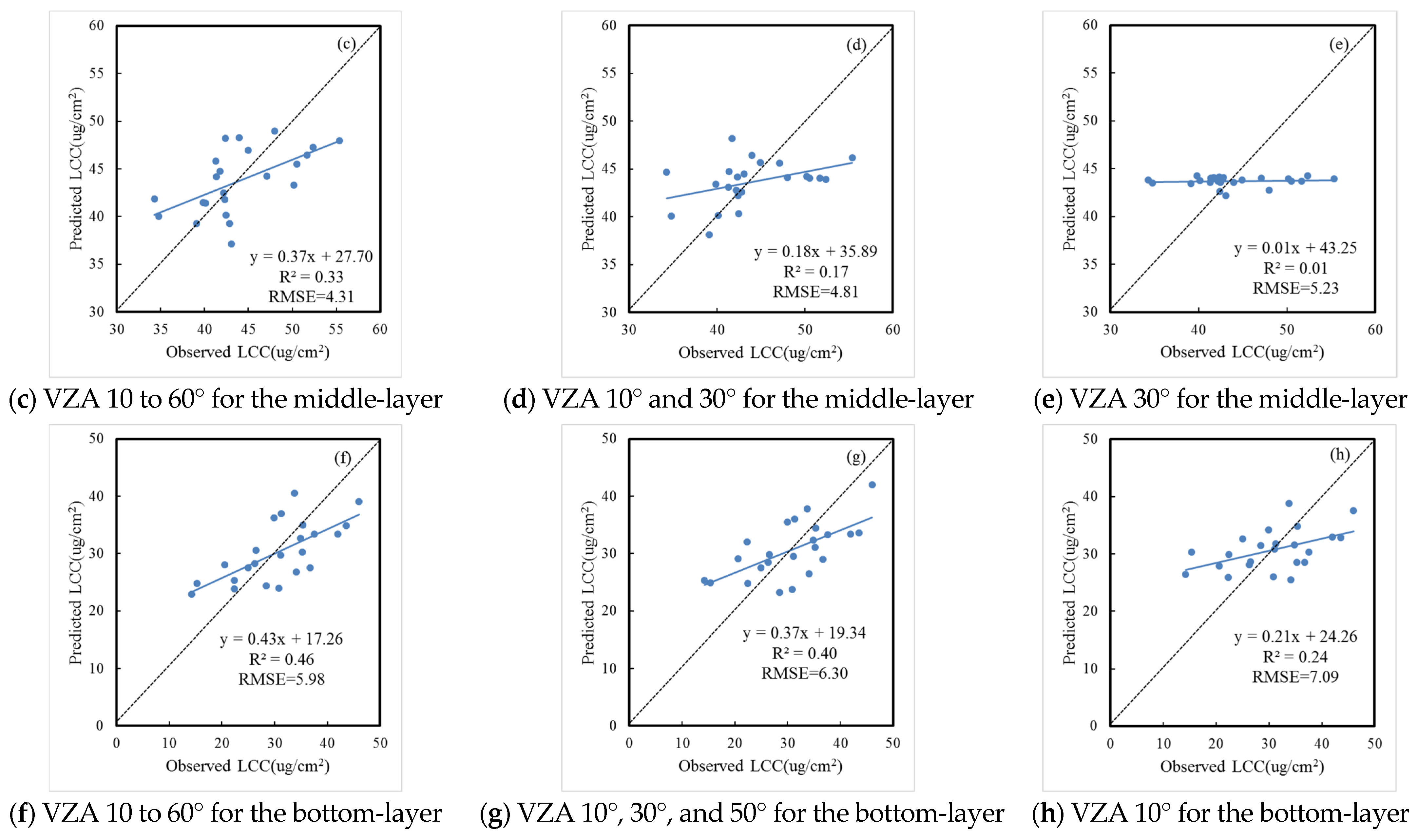
The variance analysis indicated that the VZA 10° performed best for determining the LCC of the upper-layer. For the middle-layer, the combined use of the spectral indices obtained at angles VZA 10° and 30° minimized or eliminated the influence of the upper-layer on the middle-layer. In the multivariate linear fitting results of the TCARI and MCARI/OSAVI, the spectral index coefficient of VZA 10° was negative, and that of 30° was positive, the absolute value was less than the spectral index at VZA 10°. The reason was that as the VZA increases, the contribution ratio of the LCC of the upper- and middle-layers to the spectral response spectrum decrease, whereas that of the bottom-layer increases steadily. In order to obtain an accurate result for the middle-layer LCC, it was necessary to eliminate the influence of the upper-layer. The absolute value of the coefficient reflected the change in the LCC of the middle-layer and the contribution of the LCC to the spectral response. The LCC of the middle-layer contributed more to the spectral response at VZA 30° than at VZA 10°. Multivariate linear fitting was performed for the bottom-layer LCC using the spectral indices obtained at VZA 10°, 30°, and 50°. The spectral index coefficient was negative at VZA 10° and positive at VZA 30° and 50°. This finding indicated that it is more complicated to obtain the LCC of the bottom-layer than the middle-layer. However, similar to the middle-layer, there were different degrees of contribution to the spectral response at different VZAs (10°, 30°, and 50°), which were shown in

Table 7. Leaf chlorophyll content inversion strategies for the upper-, middle-, and bottom-layers using the TCARI.

Layer	VZA Selection	Formula	R2	RMSE
Upper-layer	Single VZA	LCC = −1.76f10° + 68.42	0.58 *	5.45
	Full VZA combination	LCC = −2.69f10° + 0.68f20° + 0.55f30° − 0.03f40° + 0.07f50° − 0.12f60° + 63.25	0.61 **	5.12
Middle-layer	VZA angle	LCC = −0.14f30° + 45.79	0.07	5.18
	Optimal VZA combination	LCC = −1.40f10° + 0.33f30° + 55.43	0.35	4.81
	Full VZA combination	LCC= −1.29f10° − 0.26f20° + 0.30f30° + 0.14f40° + 0.34f50° + 0.24f60° + 47.04	0.54 *	4.26
Bottom-layer	Single VZA	LCC = 0.76f10° + 17.27	0.44 *	7.01
	Optimal VZA combination	LCC = −2.10f10° + 0.53f30° + 0.84f50° + 32.80	0.55 *	6.36
	Full VZA combination	LCC = −1.96f10° − 0.12f20° + 0.75f30° − 0.51f40° + 0.92f50° + 0.28f60° + 31.46	0.59 *	6.21

**: p value is less than 0.01, *: p value is less than 0.05.

and

Table 8. Leaf chlorophyll content inversion strategies for the upper-, middle-, and bottom-layers using the MCARI/OSAVI.

Layer	VZA Selection	Formula	R2	RMSE
Upper-layer	Single VZA	LCC = −2.05f10° + 69.19	0.68 **	4.51
	Full VZA combination	LCC = −3.71f10° + 0.89f20° + 0.90f30° − 0.44f40° − 0.23f50° + 0.25f60° + 70.27	0.79 **	3.84
Middle-layer	VZA angle	LCC = −0.14f30° + 45.58	0.09	5.17
	Optimal VZA combination	LCC = −1.11f10° + 0.32f30° + 51.05	0.31	4.90
	Full VZA combination	LCC = −1.10f10° − 0.38f20° + 0.27f30° + 0.01f40° − 0.32f50° + 0.26f60° + 47.04	0.51 *	4.47
Bottom-layer	Single VZA	LCC = 0.57f10° + 20.80	0.35	7.31
	Optimal VZA combination	LCC = −2.12f10° + 0.52f30° + 0.83f50° + 32.39	0.53 *	6.51
	Full VZA combination	LCC = −1.74f10° − 0.36f20° + 0.72f30° − 0.68f40° + 1.05f50° + 0.18f60° + 33.49	0.6 *	6.27

**: p value is less than 0.01, *: p value is less than 0.05.

.

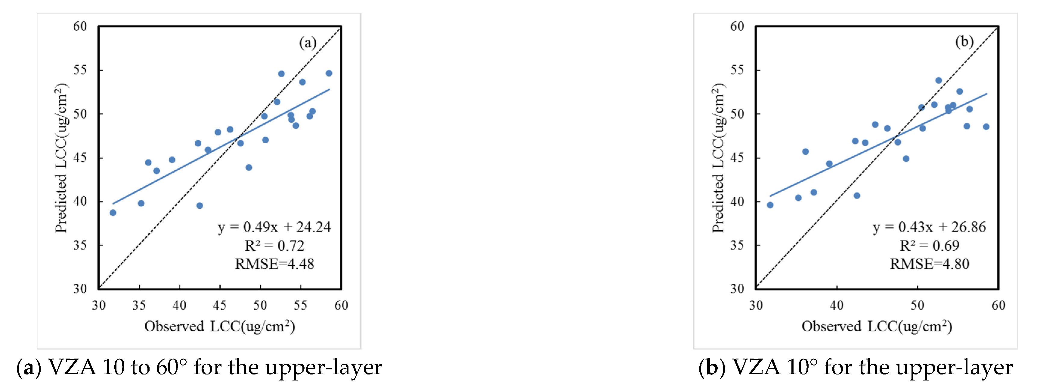
We compared two other inversion strategies to obtain the LCC of the upper- and middle-layers. The LCC of the upper- and middle-layers was obtained using a single observation angle, i.e., VZA 10° for the upper-layer and VZA 30° for the middle-layer. In addition, the LCC was obtained using all angles from VZA 10 to 60°.

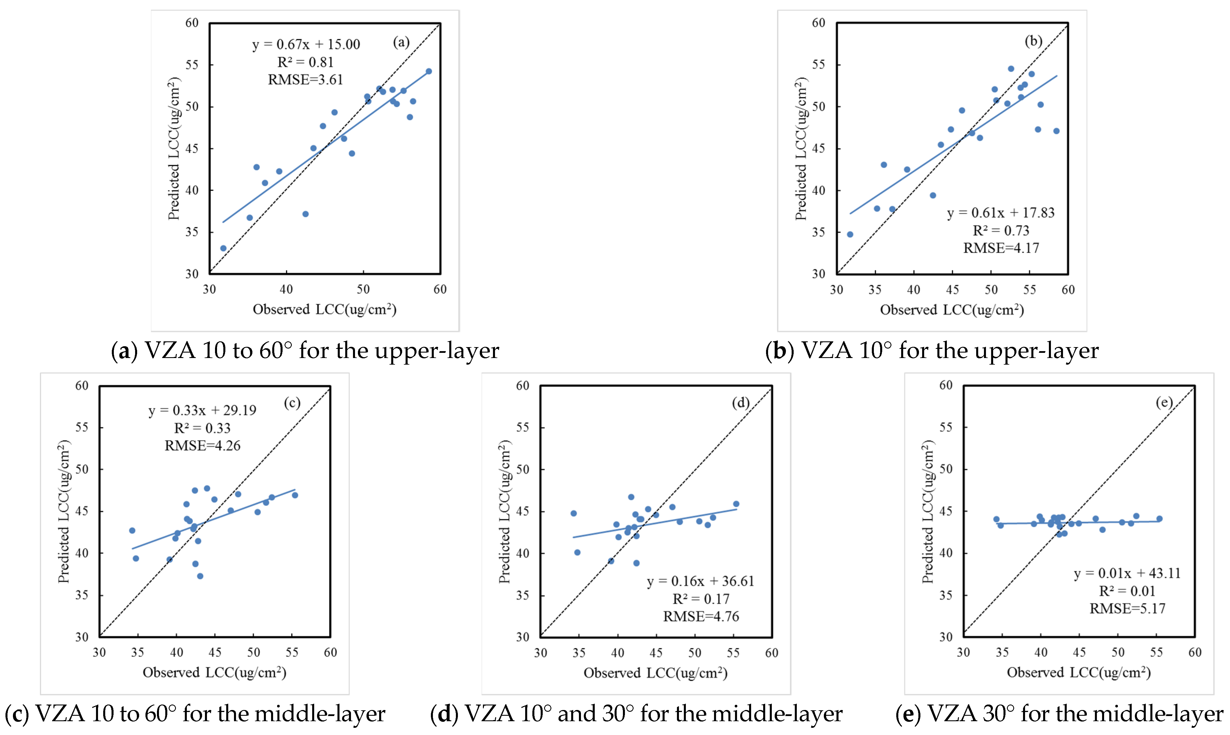
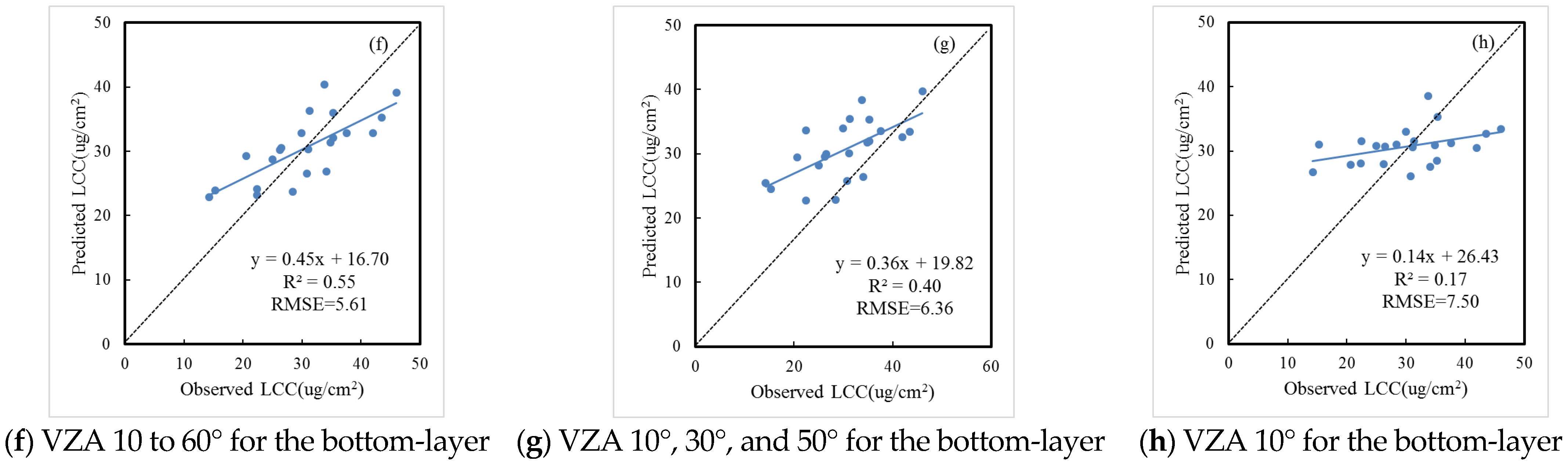
The comparison of the predicted and observed LCC based on the TCARI using different VZA combinations for the upper, middle, and bottom-layers is shown in Figure 3. The highest R² values were observed for the upper-layer (0.72 for VZA 10° to 60° and 0.69 for VZA 10°). The RMSE values were 4.48 and 4.80, respectively. The results based on MCARI/OSAVI were similar to those based on TCARI (Figure 4).

4. Discussion

Chlorophyll content in crop canopy is distributed vertically and heterogenically, and lower leaves tend to fade green and turn yellow first when crops are deficient in nitrogen. Therefore, timely and accurate monitoring of vertical distribution of chlorophyll content in crop canopy is of great significance for farmland management [37,38]. The traditional methods to obtain chlorophyll content mainly include atomic absorption spectrometry, spectrophotometry and inspection methods based on machine vision technology [37,38,39,40]. Remote sensing technology has several advantages over the traditional ground acquisition methods in obtaining and analyzing the physical and chemical parameters of crops, including timely acquisition, low cost and wide coverage, etc. Therefore, remote sensing technology has been widely used in crop growth monitoring. At present, some progress has been made in monitoring vertical distribution of crop canopy components by remote sensing. However, there is still room for improvement in both monitoring methods and monitoring accuracy [12,26]. In this study, the LCC of wheat canopy was taken as the research object, and based on canopy-scale multi-angle hyperspectral data, the optimal VZA or VZA combination of LCC at different layers was explored. The results showed that different VZA combinations were adopted to monitor the LCC at different layers (upper-, middle-, and bottom-layers), which could reduce the monitoring difficulty caused by the increase in the number of VZAs on the premise of ensuring the monitoring accuracy and was more suitable for this study.

Because of the shadowing effect of upper leaves, it is difficult to obtain the information of lower components by vertical observation [12,13,14]. Compared with vertical observation, multi-angle remote sensing monitoring can reduce the shade of upper leaves to a certain vertical layer and improve the effect of components in the lower layer of crop canopy in the spectrum, so as to improve the monitoring accuracy of LCC in the middle- and bottom-layers. However, for specific crop species (such as wheat, maize, etc.) and component characteristics (such as chlorophyll content, etc.), the observation strategy (the applicability of observed zenith angle and the applicability of observed spectral band) will change [30,32,33]. The estimated results of vertical distribution of LCC in wheat canopy leaves discussed in this study are affected by many factors when studying specific layer through spectral information (e.g., different wheat varieties, different canopy leaf stratification methods and different light conditions, etc.), especially the non-target layer leaves. In the past studies on vertical canopy distribution of crop components, similar monitoring strategies were mostly adopted for LCC at different layers (the number of observed zenith angles was the same), and the interaction between different vertical layers was ignored [12,26]. In this study, it is determined that the upper-layer adopts a single VZA (VZA50°), the middle-layer adopts a combination of two VZAs (VZA30° and VZA50°), and the bottom-layer adopts a combination of three VZAs (VZA10°, VZA30°, and VZA50°). Based on the rule that the effect of LCC at different vertical layers is constantly changing in different VZAs, the combination of VZAs can reduce the influence of non-target layers to a certain extent and improve the monitoring accuracy of the middle- and bottom-layers which are difficult to monitor. The results revealed that the proposed multi-angular observation strategy provided substantially higher accuracy of the LCC than the single-angle strategy. However, using all six VZAs gave a limited improvement in accuracy.

The TCARI and MCARI/OSAVI index used in this study are both chlorophyll sensitive indexes, which have good monitoring ability for LCC [6,35]. TCARI index and MCARI index have different band calculation methods, but they contain the same spectral bands (550 nm, 670 nm, and 700 nm). Among them, 550 nm is a strong reflection band of chlorophyll, while 670 nm and 700 nm are chlorophyll-sensitive red-edge bands. The change of chlorophyll content can cause the red edge at 670 nm and 700 nm to shift and then affect the index value. At the same time, the bands (670 nm and 700 nm) contained in the above two indices have strong penetration ability than the visible bands and are suitable for monitoring the LCC. The soil background and crop structure information in the field of view will also change with the change of VZA. The OSAVI index used in this study can weaken the influence of soil background to a certain extent [41]. It can be considered that in the case of this study, TCARI index was less affected by soil background than MCARI index, so MCARI index has a good response when combined with OSAVI index. In addition, the TCARI and MCARI index have anti-interference ability to structural parameters due to their band position and band combination form [1]. Therefore, in the monitoring of chlorophyll content in this study, the TCARI and MCARI/OSAVI index both had good monitoring ability.

However, due to limited of research resources, this article has some limitations. There may be some differences in the results of other wheat varieties and planting methods in other regions. In addition, the vertical canopy stratification method in this paper is improved compared with the stratification method in previous studies, but the change of stratification method will also affect the research results. Because the middle-layer in this study contained fewer leaves than the other layer, the response of the spectrum to this layer was poor, leading to the low accuracy of the final monitoring results (Figure 3 and Figure 4). Moreover, the current paper did not improve the optimal index form according to the wheat chlorophyll vertical distribution monitoring based on multi-angular monitoring. All the above explorations can be tried in the future research.

5. Conclusions

Remote sensing techniques are efficient approaches for the non-destructive, rapid detection of wheat LCC. The vertical distribution of the biochemical components of crops is heterogeneous, and an LCC deficit first occurs in the bottom- and middle-layers of the crop. Multi-angular observations have advantages over single-angle observations for detecting the vertical distribution characteristics of the crop’s biochemical components, overcoming the limitations of vertical observation strategies.

In this study, we analyzed the LCC in different vertical layers of winter wheat using multi-angular observations and the TCARI and MCARI/OSAVI. We analyzed the degree of information redundancy between the spectral indices for different combinations of VZAs (10°, 30°, and 50°) and determined the contribution of the LCC of different layers to the overall spectral response. Based on the results of the variance analysis, VZA 10° was used as the angle for determining the LCC of the upper-layer, VZA 10° and 30° were used for the middle-layer, and VZA 10°, 30°, and 50° were used for the bottom-layer. The result showed that the proposed multi-angular observation strategy provided substantially higher accuracy than the single-angle strategy, even when the optimal angle was used. The combination of different VZAs for monitoring the LCC of the wheat canopy minimized the influence of the non-target layer.