Abstract
In the context of the problem of image blur and nonlinear reflectance difference between bands in the registration of hyperspectral images, the conventional method has a large registration error and is even unable to complete the registration. This paper proposes a robust and efficient registration algorithm based on iterative clustering for interband registration of hyperspectral images. The algorithm starts by extracting feature points using the scale-invariant feature transform (SIFT) to achieve initial putative matching. Subsequently, feature matching is performed using four-dimensional descriptors based on the geometric, radiometric, and feature properties of the data. An efficient iterative clustering method is proposed to perform cluster analysis on the proposed descriptors and extract the correct matching points. In addition, we use an adaptive strategy to analyze the key parameters and extract values automatically during the iterative process. We designed four experiments to prove that our method solves the problem of blurred image registration and multi-modal registration of hyperspectral images. It has high robustness to multiple scenes, multiple satellites, and multiple transformations, and it is better than other similar feature matching algorithms.
1. Introduction
Hyperspectral remote sensing imaging, as an important means of remote sensing for earth observation, has been widely used due to its powerful ability to finely divide ground objects. Hyperspectral image processing has become one of the hot spots in imaging technology and application fields in recent years. Interband registration of hyperspectral imagery is required for different applications. The registration accuracy significantly affects the image fusion results, target recognition, scene reconstruction, and other applications; therefore, an accurate interband registration algorithm is required.
Traditional image registration methods can be divided into three categories: (1) area-based registration, (2) feature-based registration, and (3) learning-based registration. Area-based registration methods register the two images according to the grayscale or domain conversion information in a sliding window of a predefined size, or a similarity metric is used for the entire image. This method has good registration accuracy for normal scenes. Feature-based registration methods extract and describe the feature points based on the local grayscale or contour information of the image. The feature points are matched according to the similarity of the descriptors to achieve image registration. This method has relatively good scene adaptability but has high requirements for the distribution and accuracy of the feature points. Learning-based registration methods use neural networks to extract deep features of the image. When the model training data are adequate, this method often provides better registration results than conventional methods.
The wavelength range of most hyperspectral images covers the visible and near-infrared bands. The registration of visible and near-infrared band images is a challenging task. As shown in Figure 1b,c, the two images show significant nonlinear reflectance differences, the grayscale values change and the wavelength change are not linearly related, and the grayscale values of the same features are very different. As a result, the use of features based on grayscale information is unreliable, significantly increasing the difficulty of band registration.
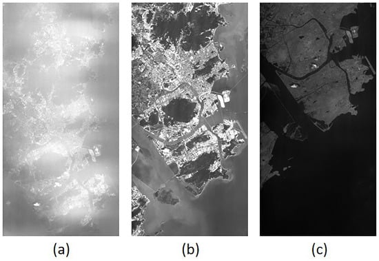
Figure 1.
Three bands of an Orbita Hyperspectral Satellite (OHS) image. (a) is the 1st band, with a center wavelength of 466 nm; (b) is the 15th band, with a center wavelength of 686 nm; (c) is the 32nd band, with a center wavelength of 940 nm.
Due to a large number of spectra in hyperspectral images and the narrow spectral bandwidth, the instantaneous field of view (IFOV) is not sufficiently large to collect enough photons [1]. Thus, the hyperspectral images in the lower wavelength band have lower light energy, resulting in image blur, which is especially pronounced in the 1st band, as shown in Figure 1a. The contour of the blurred image is relatively low, decreasing the accuracy of contour-based features and band registration accuracy.
Given the hyperspectral image characteristics, we propose an adaptive iterative clustering feature matching method for fast and accurate interband registration of hyperspectral images. This method uses a four-dimensional descriptor based on geometric, radiometric, and feature information to obtain a putative match. This descriptor improves the putative match from multiple angles so that the image can be accurately described, even if some of the characteristics are lost. We perform principal component analysis on the four-dimensional descriptors and use the three principal components with the largest weights to create a new three-dimensional descriptor for simplification. The three-dimensional description allows for easy data visualization to evaluate the results of putative matching. Finally, an iterative clustering method is used for feature matching of the three-dimensional descriptor to obtain a correct match. We analyze the key parameters in the iterative clustering so that the values are chosen adaptively during the iterative process. This strategy provides a robust method for the iterative processing of the different bands. The proposed method has higher registration accuracy than other feature matching methods.
The main contributions of this study are three-fold. First, a four-dimensional descriptor with geometric, radiometric, and feature information is proposed based on the hyperspectral image characteristics. This descriptor allows us to describe low-precision putative matches when part of the image information is unreliable. Second, we perform principal component analysis on the four-dimensional descriptors to reduce it to three dimensions. An adaptive iterative clustering method is used to obtain correct matching feature points. Finally, we use thin-plate spline (TPS) interpolation to transform and register the band images. The algorithm performs the feature matching task with O(N) time complexity, which is of great significance for the implementation of batch interband registration or on-board orbit registration in the future. The proposed method has several advantages over similar methods in terms of feature matching and image registration, especially for data with a high outlier rate.
The rest of this article is organized as follows. Section 2 introduces the background material and related work. In Section 3, we introduce the hyperspectral images band registration algorithm based on adaptive iterative clustering. Section 4 presents the matching and registration performance of the proposed method and other methods and summarizes the advantages and limitations of our method. Section 5 provides the conclusion.
2. Related Works
Feature-based methods often show better multi-scene adaptability and anti-interference ability than other image matching methods and are currently mainstream registration algorithms. Therefore, we focus on feature-based image registration algorithms. The process is generally divided into three steps: feature extraction and description, feature matching, and transformation. The first step can get the putative matching, and the second step removing mismatches. In this section, we describe some classic algorithms and the latest algorithms used for the two steps.
For the first step, many classic algorithms have been widely used for image registration, such as scale-invariant feature transform (SIFT) [2], speeded-up robust features (SURF) [3], and oriented brief (ORB) [4]. The SIFT algorithm is the most common method used for image local features. It extracts extreme points in the difference of Gaussian (DOG) scale space and optimizes them to obtain the feature points. SIFT has rotation invariance and scale invariance and strong adaptability to lighting and viewing angle changes. SURF uses integral images and the Hessian matrix and Harr wavelet to accelerate the SIFT algorithm for feature extraction and description, respectively. The ORB algorithm is a new corner detection and feature description algorithm that combines features from accelerated segment test (FAST) corner detection and binary robust independent elementary features (BRIEF) feature description, making it rotation-invariant and robust to noise. However, these classic methods still have some problems. For example, in a multi-modal scene, two images may have relatively large reflectance differences, leading to a high mismatch rate of the feature points extracted by traditional methods and low registration accuracy. The histogram of oriented gradients (HOG) [5] is a descriptor that characterizes the local gradient direction and gradient intensity of an image. The HOG was improved using the channel features of orientated gradients (CFOG) [6] and histogram of orientated phase congruency (HOPC) [7], which use gradient information or orientated phase congruency to capture the geometric or shape characteristics of the image. The methods are suitable for multi-modal image registration, but they have a high mismatch rate and high algorithm complexity, which is very time-consuming.
Due to various problems in feature extraction in the first step, a relatively low number of inliers are obtained in the putative match. Therefore, many methods have been proposed to eliminate mismatches in the second step. The random sample consensus (RANSAC) [8] is a classic mismatch removal algorithm. It uses several assumptions and verification strategies to find the smallest consistent internal set to fit a given geometric model. RANSAC has many variants; for example, the maximum likelihood sample consensus (MLESAC) [9] is a generalization of RANSAC based on probabilistic interpretation. GroupSAC [10] uses prior values so that the inliers are more similar to improve the sampling phase. The locally optimized RANSAC (LORANSAC) [11] and the fixed LORANSAC (FLORANSAC) [12] assumes that the model fitted by the non-outliers is consistent with all outliers. These methods locally optimize the model based on the current inlier set. Chum and Matas proposed a model verification strategy called a modified sequential probability ratio (SPR) [13] test to reduce the time complexity. However, the initial outlier rate is usually higher than 95%. With such a high rate of outliers, RANSAC and its variants require many subset sampling tests to obtain satisfactory results, significantly reducing efficiency [14].
Non-parametric methods include the linear adaptive filtering (LAF) [15], locality-preserving matching (LPM) [16], mTopKRP [17], locally linear transforming (LLT) [18], and robust feature matching based on spatial clustering of applications with noise (RFM-SCAN) [19]. The LAF transforms the feature matching problem into filtering and denoising problems using Gaussian convolution operations and gridding, progressive or iterative strategies, and parameter adaptation strategies to achieve feature matching with linear time and space complexity. The LPM uses local neighborhood information to find a consistent match, which greatly improves the matching speed. The mTopKRP improves the performance of the LPM by using a k-nearest neighbor (K-NN) ranking list derived from local neighborhood information. The LLT creates a set of hypothetical correspondences based on feature similarity, removes the outliers based on the correspondences, and estimates the transformation. Feature matching can still be achieved for a large number of outliers (up to 80%). The RFM-SCAN transforms the feature matching problem into a spatial clustering problem with outliers.
Note that the RFM-SCAN also uses spatial clustering to eliminate mismatches. However, there are several differences between this method and our proposed method. (1) The RFM-SCAN only uses motion vectors to describe putative matching, whereas our method uses four-dimensional descriptors that consider the geometric, radiometric, and feature information of the hyperspectral images. (2) The RFM-SCAN uses the classic density-based spatial clustering method (density-based spatial clustering of applications with noise, DBSCAN [20]), while our method uses the centroid-based k-means as the spatial clustering method based on the four-dimensional descriptor. (3) The objectives of the two methods are different. The RFM-SCAN focuses on image retrieval and joint segmentation, whereas the objective of our method is image registration. As described in Section 4, our method provides better matching accuracy than the RFM-SCAN.
In recent years, deep learning has continued to develop, and several learning-based methods have emerged, such as learning to find good correspondences (LFGC) [21] and NM-Net [22]. LFGC is the first algorithm using a PointNet architecture to establish a deep learning framework based on multi-layer perceptrons to eliminate outliers. NM-Net improves LFGC by adding local information obtained from compatibility-specific proximity mining algorithms to the deep learning framework. Wang et al. [23] paired the small blocks in the perception image and the reference image and then directly learned the mapping between these small block pairs and their matching tags and then performed registration. Zhang et al. [24] proposed OANet(Order-Aware Network), which can infer the corresponding probability and return to the relative pose encoded by the essential matrix. The network is divided into three layers and intensively performed on both outdoor and indoor data sets. Experiments have achieved good results. However, these methods require data training, and the trained models have low adaptability to different scenarios or multi-modal registration, limiting their practical use.
3. Method
This section introduces the details of the proposed interband registration method based on iterative clustering. The algorithm starts by extracting the putative matches using SIFT, followed by developing suitable matching descriptors and obtaining the correct matching points through cluster analysis of the descriptors. Subsequently, we fit the transformation function from the original image to the target image using limited and relatively uniformly distributed matching points to complete the registration.
3.1. Problem Formulation
Given the original image and the target image, the initial n pairs of the putative matches are obtained after using SIFT to extract and match the feature points , where and , and are the feature points of the original image and target image, respectively. There are two reasons why we use SIFT to extract putative matching: (1) Compared with algorithms such as SURF, although SIFT has a slower operation speed, it can extract relatively more initial matches to adapt to the hyperspectral image with low inlier rate. (2) In the original papers of the comparison method of our experimental chapter, SIFT is used to extract the putative matching, and we use the same algorithm to control the variables. Due to the blurred and multi-modal characteristics of the hyperspectral images, the putative match set S usually contains some mismatched points, significantly affecting the final fitting transformation function and causing registration failure. For this reason, we assume that the outliers in the S set are randomly and uniformly distributed [9]. In this way, the matching problem is transformed into finding the inlier set I in the S set with randomly and uniformly distributed outliers.
Clustering is a process of dividing a set into several clusters, and the points in each cluster have greater similarities [25]. Clustering is an unsupervised classification process; i.e., points with similar characteristics are grouped into a cluster without parameters. In clustering, high-dimensional data are mapped to a high-dimensional geometric space. Due to the sparse nature of the data, many data points are distributed in their respective hyperplanes. Generally, the points that are distributed in the same hyperplane have greater similarity; in the same hyperplane, the smaller the geometric distance, the greater the similarity is. Clustering is used to complete the matching task, i.e., to find a suitable descriptor to describe each pair of putative matches , which are used to map the set S to a high-dimensional space. Subsequently, a suitable clustering algorithm is used to divide S into several clusters, and the cluster with the inlier set of interest is located so that the correct matching points are obtained. The entire process of interband registration is shown in Figure 2. The following conditions are required to transform the problem: (1) the proposed descriptor should be as close as possible to the true distribution of S; (2) The attributes of the inliers should be sufficiently similar to be divided into a cluster.
| Algorithm 1: Feature matching based on iterative clustering |
| Input: Inferred matching set: S, initial value of k: k, the maximum number of iterations: max |
| Output: Output: inlier set: I |
| 1: Calculate using Equation (1) |
| 2: Calculate using Equation (2) |
| 3: Calculate using Equation (3) |
| 4: Combine , and into a four-dimensional descriptor |
| 5: Use principal component analysis to reduce the four dimensions to three dimensions |
| 6: Iteration: |
| 7: Start k-means using the initial value or the k value obtained from the last iteration |
| 8: Count the number of points in each cluster and calculate in the clustering result |
| 9: Calculate the value of k in the next iteration using Equation (11) |
| 10: The cluster with the largest number of points forms the point set I |
| 11: Until decreases for the first time or the number of iterations>max |
| 12: Return I |
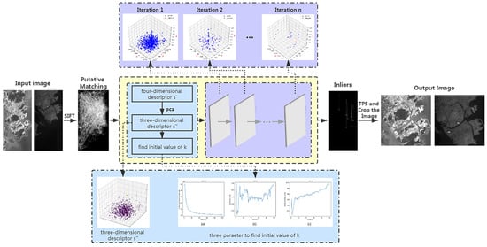
Figure 2.
The proposed adaptive interband registration framework based on adaptive iterative clustering. The main body is illustrated in the second row. We get putative matching from the input image pair through the scale-invariant feature transform (SIFT) algorithm. Then, we enter the yellow flow diagram, which is Algorithm 1. It contains two parts: preprocessing (blue diagram) and adaptive iterative clustering (purple diagram). After the iterative clustering reaches convergence, the cluster with the largest number of points is obtained, which is the inliers. From the inliers, the thin-plate spline (TPS) algorithm is used and the image is cropped to obtain the output image pair. Among them, the first row is a visual image to supplement the iterative clustering process; the third row is a visual image to supplement the preprocessing process.
3.2. Establishment of the Four-Dimensional Descriptor
Due to the hyperspectral image characteristics, we need to find a complete description of the attributes. The geometric, radiometric, and feature attributes are used.
Because the images in the lower wavelength of the hyperspectral images are blurred, it is difficult to accurately describe the geometric attributes of each pair of putative matches in the registration between those bands. However, in the registration of the hyperspectral images in the visible and near-infrared bands (multi-modal), the description of the geometric attributes is crucial. The inliers in S always have a smooth and regular distribution and geometric consistency. We select the motion vector of each pair of feature points as the description of the geometric attributes:
In Figure 3, the motion vectors of putative matches constitute the entire image of the motion field. The motion vectors of the inliers are always smooth and regular (Figure 3d), while the motion vectors of the outliers are randomly distributed (Figure 3c).
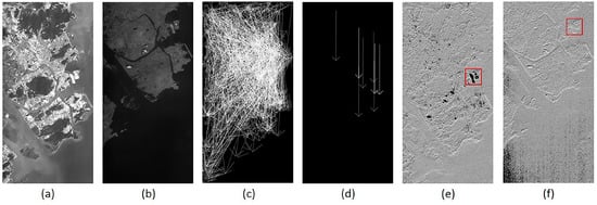
Figure 3.
The original image (32nd band) and target image (15th band) of the OHS image and its motion field and gradient direction. (a,b) are the 15th band and 32nd band images, respectively; (c) is the putative matching motion field from the original image to the target image, that is, the set of all feature points from the original image to the target image, and it contains many outliers; (d) is the motion field of the inliers, which is detected manually and which is the ground truth of this experiment; (e,f) are the gradient patterns of the 15th band and the 32nd band, respectively; the grayscale values represent the gradient direction of the point.
The visible waveband and near-infrared waveband have different spectral responses for the same object, and there are significant nonlinear reflectance differences; thus, the grayscale-based features are unreliable. As shown in Figure 3e,f, the red frame represents the same object in the two bands, but the grayscale values are very different; i.e., the gradient direction is very different. A reverse gradient may occur, and the gradient size of the inliers is also irregular. However, the problem can be solved by representing the grayscale information in two images. We propose as a descriptor of the radiometric properties. It is defined as:
where represents the number of pixels in the target image with the same gray value as , represents the number of pixels in the original image with the same gray value as , col1 and row1 represent the number of columns and rows of the target image, and col2 and row2 represent the number of columns and rows of the original image. In the interband registration of the hyperspectral images in this study, the size of the target image and the original image are the same. In this way, the and in a pair of putative matches are calculated in the grayscale ratio in the respective images. This straightforward method prevents the problem of nonlinear reflectance differences in multi-modal registration. However, since the overlap between the original image and the target image is not 100%, the descriptor has an error. In theory, the smaller the overlap, the greater the error is. In the registration between the hyperspectral images of our experiment, the degree of overlap of the band images is more than 70%. In addition, in the principal component analysis, the dimensionality reduction process gives low weights for the descriptors with large errors. Therefore, the error caused by the descriptor is within an acceptable range.
In the SIFT algorithm, it comes with a quantity that characterizes the matching degree of feature points:
where represents the closest distance between the target image feature point and , and represents the next closest distance between the feature point of the target image and . The distance is the Euclidean distance:
where n represents the spatial dimension. measures the degree of feature matching of each pair of feature points in the putative matching. The smaller the , the better the degree of feature matching is.
In this way, the putative matching set is transformed into the new description , where the motion vector is two-dimensional, so is a four-dimensional descriptor that considers the geometric, radiometric, and feature attributes of hyperspectral images. The following verification shows that the four-dimensional descriptor we proposed is highly robust to hyperspectral images geometry and radiometric distortion.
3.3. Iterative Clustering
We performed the principal component analysis for the following three reasons to reduce the dimension of the proposed four-dimensional descriptor, and we selected the first three components with the largest weight to create a new three-dimensional descriptor , which forms the set . (1) There is data sparsity in a high-dimensional space. Many similarity measures are not applicable to a high-dimensional space. In addition, the number of subsequent operations will increase exponentially as the dimension increases. This phenomenon is referred to as the curse of dimensionality [26]. Aggarwal et al. conducted an in-depth study on the relationship between the LK norm and the data dimension. The results showed that the difference between the nearest neighbor and the farthest neighbor decreased with increasing dimension, and the distance contrast between points no longer exists [27]. (2) As mentioned above, an error in the occurs because the original image and the target image do not have a 100% overlap. Dimensionality reduction can reduce the mapping weight of the to reduce errors. (3) The assessment of the distribution of the inliers and outliers in the putative matching is facilitated by reducing the four-dimensional descriptor to a three-dimensional descriptor. As shown in Figure 4, the inliers (yellow) are uniformly distributed.
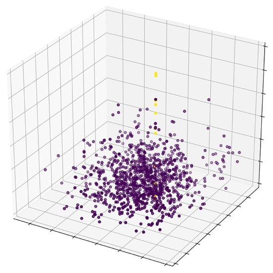
Figure 4.
The spatial distribution of putative matches three-dimensional descriptors. The three coordinate axes are the mapping of the four dimensions, which have no specific meaning. The yellow points are the inliers, which are detected manually, and the purple points are the outliers.
In the principal component analysis, we regard as n four-dimensional data. First, is transformed into a matrix X of 4 rows and n columns, and each row of X is zero-averaged to obtain the covariance matrix . The eigenvalues of the modified covariance matrix and the corresponding eigenvectors are obtained, and the eigenvectors are arranged in a matrix from top to bottom according to the size of the eigenvalues. We use the first three rows to create the matrix P so that to obtain the new three-dimensional descriptor .
The standard clustering algorithms include centroid-based clustering methods, such as k-means [28] and k-modes [29]; hierarchical clustering methods, such as Chameleon [30] algorithm; density-based clustering methods, such as DBSCAN; and model-based clustering methods Clustering methods, such as EM [31] and SOM [32]. Different clustering methods are suitable for different data distributions. The registration of the hyperspectral images bands is challenging due to the blurred images and multiple bands. The number of data points in the putative matching set of the hyperspectral images is relatively low, and the proportion of inliers is small, generally less than 10%. In addition, the number of inliers is low, and the distribution is relatively concentrated, whereas the outliers are randomly and uniformly distributed. Theoretically, the density-based clustering method is suitable for this data distribution, but it is difficult to achieve high-dimensional data clustering. The k-means algorithm is the most common clustering algorithm. It is straightforward, highly efficient for processing large data sets, and has good scalability. More importantly, in order to speed up the convergence speed, our method iterates the clustering method. From the perspective of saving running memory and running time, k-means is the best choice. Thus, we use the iterative k-means algorithm to achieve rapid convergence. In detail, in one iteration, the algorithm randomly selects k centroids in the three-dimensional Euclidean space, assigns each point in to the closest centroid, and calculates the mean of the points in each class as the updated centroid. The points of are then re-distributed according to the new centroid distance. The process is repeated to update the center points and assignments until all points are assigned or the maximum number of iterations is reached. After entering n points to perform k-means clustering, the inliers are often in the cluster with the largest number of points (the number of points is ). Let , where is the number of inliers, which are manually verified in the putative match. At this time, is very small, indicating that a single cluster cannot extract the inliers. Therefore, we designed an iterative clustering process that uses the cluster with most points after one iteration as the input to the next iteration. As shown in Figure 5, the number of points in each iteration is continuously reduced. In each iteration, we calculate the ratio of the number of points of the largest cluster to the number of input points , where , and is the number of input points of this iteration. The ratio increases with the number of iterations. When the value of decreases for the first time, the clustering performance is lower than the previous one, but reaches the maximum value for feature matching. The cluster with most points represents the inlier set output by the algorithm. Therefore, the algorithm has converged when the value decreases for the first time.
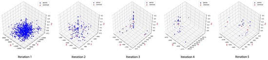
Figure 5.
Scattered point distribution during iteration. The blue dots represent all the data in the iteration; the red dots represent the centroids of the clusters. As the number of iterations increases, the number of putative matches decreases, the input point set approaches the inlier set, and the number of clusters divided by each cluster is also decreased accordingly.
As an unsupervised classification algorithm, the k-means algorithm learns from the unlabeled training samples to determine the structure of the training sample set. The algorithm has no additional parameter settings. The only parameter is the number of clusters (k). The value of k significantly affects the clustering results. The selection of the k value is based on the data distribution and experience. The elbow method and the contour coefficient method were developed to select the k value. The proposed algorithm is an iterative k-means algorithm; thus, multiple k values are required. Experiments were conducted to achieve the adaptive selection of the k value. In detail, during clustering, the variable closely related to the value of k is , which is the ratio of the maximum number of cluster points to the number of input data. This parameter affects the number of clusters (k) created in the next clustering step. The adaptive selection of k is achieved using two processes: (1) the selection of the initial value, and (2) the adaptation in the iterative process.
It can be seen from Figure 6 that the initial k will greatly affect the accuracy of our method. In addition, it can also be seen that a single clustering is not enough to find the inliers with a low inlier rate, so an iterative clustering process is required. We perform an initial clustering of the data with a certain value of k and analyze the results. Three evaluation indicators are used. The first is the average contour coefficient (silhouette_score, s_s) [33]. A higher profile coefficient score indicates a better clustering model. A contour coefficient is defined for each sample and consists of two scores. a is the mean distance between a sample and all other points in the same class (cohesion), and b is the mean distance between a sample and all other points in the next nearest cluster (dispersion). The profile factor s_s of a single sample is given as:
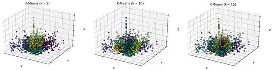
Figure 6.
The first clustering results of three-dimensional descriptors with different initial k. From left to right are the clustering results of k = 5, k = 10, and k = 15, respectively.
The definition of the nearest cluster is
where p is a sample in a given cluster . The average distance of all samples from point to a given cluster is the measure of the distance from the point to the cluster, and the cluster closest to is selected as the closest cluster. The s_s is used. It has a range of [−1, 1]; the closer the sample distance in the cluster, and the farther the sample distance between the clusters, the larger the s_s is, and the better the clustering performance is. The second indicator is the Calinski–Harabasz score (ch_s) [34], which is the ratio of the sum of the between-cluster dispersion and the inter-cluster dispersion for all clusters, where the dispersion is defined as the sum of the distances squared. For a set of data E of size , which has been clustered into k clusters, the ch_s is defined as:
where and are the traces of the group dispersion matrix and the intra-cluster dispersion matrix, respectively, which are defined as:
where is the point set in cluster q, is the center of cluster q, is the center of E, and is the number of points in cluster q. A higher ch_s indicates that the clusters are dense and well separated. The third indicator is the inertia score (i_s), an attribute of the k-means model object. It represents the sum of the nearest cluster center of the sample. It is used as an unsupervised evaluation indicator and has no classification labels. The smaller the value, the better the performance is, the more concentrated the samples distribution between clusters, and the smaller the distance within the class is. The above three indicators are used to analyze the clustering results after the first k-means. The results are shown in Figure 7. The s_s indicator (Figure 7b) decreases significantly from 2 to 3 and then gradually increases. When k = 11, the s_s reaches the maximum value; as the k value increases further, the fluctuations of the score are small. The ch_s (Figure 7c) shows a similar trend. The value first drops sharply as the value of k increases and then rises sharply. When k = 11, the score reaches a local maximum and then increases slightly. The change in i_s (Figure 7a) is relatively smooth. First, it decreases sharply as the value of k increases. When k = 11, the rate of decrease gradually decreases, and then the slope approaches 0. The k value of the k-means algorithm should not be very large because the relevance of the data is reduced. Based on the results of the three indicators, we set the initial k value to 11. The subsequent experiment indicates that this value of k is appropriate.
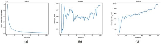
Figure 7.
The results of the indicators i_s (a), s_s (b), and ch_s (c) for k-means clustering.
We determine which of the independent variables (, i_s, s_s, and ch_s) may affect the value of k to ensure that the value of k is chosen adaptively in the iterative process. Then, we choose an initial value of k in the first step to obtain a large data set of the dependent variable k and the four independent variables. In the second iteration, we calculate the optimal value of the three indices (i_s, s_s, and ch_s) of k for different values of k and obtain the i_s, s_s, and ch_s. The optimal k value and the values of the four independent variables are obtained during each iteration. We use Spearman’s rank correlation coefficient to calculate the nonlinear correlation between k and the independent variables. We select as the only independent variable of k and determine the distribution of k and . The distribution shows the following inversely proportional relationship between k and :
where k1 is the slope, and b1 is the intercept. The gradient descent method is used to perform one-variable nonlinear fitting with a large number of k and values. The results show that k1 = 3.637 and b1 = −0.697. Since the proportion of inliers increases as the iteration progresses, the value of k should not theoretically increase during the iteration process. In summary, the empirical formula of k obtained from the iterative process is:
where is the k value of the last cluster, min() is the minimum value function. In this cluster, we use the minimum of and k value calculated according to . The minimum k becomes the k value of the next cluster for an adaptive selection of the k value.
3.4. Registration and Time Complexity Analysis
After obtaining the inlier set I, we calculate the transformation matrix from the original image to the target image. The proposed interband registration is a rigid transformation, but we want it to retain the potential of non-rigid transformation. We choose the TPS interpolation method to calculate the transformation parameters, which are generality and smooth function mapping properties in supervised learning [35]. We use TPS to calculate the transformation function F, , where is the vector defined by the TPS kernel. The parameter A controls the global linear affine motion component of the transformation, and the parameter H controls the local nonlinear affine motion component. After the nonlinear space mapping function F is obtained, the coordinates of the pixels in the original image are calculated using F, and the gray values of the points are calculated using bicubic linear interpolation to complete the regstration.
The time complexity of a single k-means iteration is O(N). However, we added an external iterative process. Due to our iterative clustering input and output settings and the adaptive selection of the k values, convergence occurs within 6 iterations. Therefore, the number of external iterations relative to the number of samples N is negligible. Thus, the time complexity of the proposed feature matching algorithm is O(N), and the feature matching task can be completed in a few hundred milliseconds, allowing for future batch processing and on-board processing.
3.5. Implementation Details
In principle, the cluster with the inliers should be the cluster with the most points due to the high similarity between the inliers, the small geometric distance, the random and uniform distribution of the outliers, and the use of a suitable value of k. The subsequent experiments validate this assumption. In summary, we can use the largest cluster in one iteration as the input of the next iteration, which is applicable in theory and practice. In addition, when the iteration converges, the number of output inliers may vary significantly and is closely related to the registered image. If there are many inliers, the TPS interpolation will require a long time. Thus, we set the threshold M. When the number of inliers is greater than M, we randomly shuffle the order of the inliers and use the first M points as the input of TPS. Thus, the calculation time is reduced without affecting the accuracy of the registration. In addition, by randomly changing the order of the inliers, the points used in the transformation estimation are randomly distributed in the original image. This approach reduces the registration error caused by the excessive clustering of the feature points. Experiments showed that a value of 10 for M met our registration requirements. It is also worth noting that is the number of inliers in the . This value is calculated manually and is only used for analysis and reference. The algorithm does not require this value.
4. Experimental Results
In this section, we describe four experiments that we designed to verify our method. (1) Multi-scene interband registration using OHS data as an example. We used 60 sets of OHS data for interband registration. These 60 sets of data contained as many artificial and natural features as possible. This experiment is used to verify the robustness of our method to various ground object scenes. (2) Interband registration of seven kinds of hyperspectral (multispectral) satellite data: we used OHS, ZY-1E, EO-1, Terra, GF-2, Sentinel-2, and Landsat7 data. For each type of satellite, 10 sets of interband registration experiments were been done, and the ground resolution and map size of each group of experiments have increased differences. This experiment was used to verify the robustness of our method to various data. (3) Multi-method feature matching and interband registration comparison experiment using OHS data as an example. We compare with the most classic RANSAC and the latest feature matching algorithms LPM, LLT, mTopKRP, RFM-SCAN. The above methods all use the original parameters of their paper. This experiment is used to verify the superiority of our method over other similar methods. (4) Supplementary experiments for adding rotation, scaling, and noise, taking OHS data as an example. We artificially add rotation and scaling transformations for interband registration to verify the robustness of our method to various transformations. In addition, we perform interband registration on images with added salt noise to verify the robustness of our method to noise. All experimental OHS data were pre-processed before interband registration in our previous work [36], including decoding, radiation correction, framing, etc. All the following experiments are run on a personal computer with Inter(R) Core(TM) i5-6300HG CPU @ 2.30 GHz 2.30 GHz and 8 GB RAM. We will open source python code of the proposed method: https://github.com/RuizJoker/Adaptive-Iterative-Clustering (accessed on 1 June 2020).
4.1. Multi-Scene Interband Registration of Hyperspectral Images
We randomly selected several remote sensing scenes of the hyperspectral images to ensure the applicability of the proposed method in various scenarios. The experimental results are shown in Figure 8, where the top left feature scene is a city, the top right feature scene is a lake, the bottom left feature scene is a farmland, and the bottom right feature scene is a mountain. The data show nonlinear reflectance differences between the bands. We have specially selected pixel-level pictures with regular-shaped objects. The results indicate good registration accuracy at the pixel level.

Figure 8.
Interband registration results between four sets of hyperspectral image. In each set result, the first row from left to right shows the 1st, 8th, 15th, 24th, and 32nd bands of the original images of the hyperspectral images; the second row shows the registered and cropped images; the third row and the fourth row show the registration details of the 1st, 8th, 24th, and 32nd bands relative to the target image (the 15th band). A scene with unique features is selected and magnified to the pixel level to show the registration accuracy. The target image is inside, and the original image is outside the rectangular frame.
4.2. Interband Registration Experiment between Multiple Remote Sensing Image
We used 20 sets of hyperspectral (multispectral) data each of OHS, ZY-1E, EO-1, Terra, GF-2, Sentinel-2, and Landsat7 for testing. We selected two representative experiments to displas the result of the interband registration for each type of satellite data. For the selected experimental data, we chose the farthest band image for testing as much as possible to ensure the non-linear radiation difference across the band; in addition, the 14 sets of experimental data displayed have different ground resolutions and different map sizes. Table 1 shows the specific parameters of each group of experimental data.

Table 1.
14 sets of experimental data specific parameters.
The interband registration results of the 14 sets of experimental data are shown in Figure 9. We have added the checkboard results of the original image and the registered image, and we can intuitively see the registration effect. It can be seen that our method has a good registration effect for each kinds of hyperspectral (multispectral) remote sensing data. In particular, in the motion field before registration, we can see that the distribution of motion vectors is messy, and our method can extract a set of feature points with the highest similarity in the putative matching. Therefore, in the motion field after registration, the motion vectors are distributed regularly. In addition, there is a large quantity difference in the putative matching points of each group of images. In order to make the motion field image more beautiful, we adjusted the length and width of the vector line segment differently according to the number.
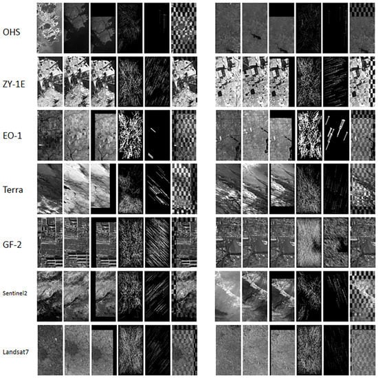
Figure 9.
Interband registration results of 14 sets of experimental data. Each row shows one type of satellite data, and each row shows two sets of experiments. In each set of registration results, from left to right are the target image, the original image, the registered image, the putative matching motion field, the motion field of feature points after the feature matching, and the combined checkboard results of the target image and the registered image.
4.3. Comparison of Different Algorithms
Due to the single object type of some images, such as deserts and oceans, combined with the influence of blurred and multi-modal registration, it is difficult to find a sufficient number of correct feature points in the putative matching after SIFT. Therefore, we chose images with many typical objects and obvious features for comparing the different algorithms. We used the 15th band and 32nd band registration to perform feature matching and interband registration. We manually verified all feature point pairs in putative match; 12 pairs of the matches (1096 pairs) were inliers, and the inlier rate was only 1.09%.
The F-score can characterize the comprehensive performance of feature matching. We used the F-score and running time as the evaluation criteria for feature matching. The F-score is defined as . In addition, we used the root mean square error (RMSE), mean average error (MAE), and minimum error entropy (MEE) as evaluation indicators for interband registration:
where are the image coordinates of the feature point of the target image in the obtained matching result, are the image coordinates of the feature point of the original image in the obtained matching result, F is the conversion function, I is the number of feature points, max() is the maximum value function, and median() is the median function.
4.3.1. Feature Matching
Figure 10 shows the feature matching results of RANSAC, LPM, LLT, mTopKRP, RFM-SCAN, OANet and the proposed method. Table 2 lists the quantitative results of the feature matching of the seven methods. Among them, if RANSAC is to traverse all the situations, it will be very time-consuming, so the upper limit of iteration will be set in actual use, which greatly limits the accuracy of its results. It can be seen from Table 2 that the five points obtained by RANSAC were all outliers, and the precision and recall rate were both 0%. The LPM and LLT provide low performance. There were only five pairs of inliers in the extracted feature points, the precision was only 6.10% and 1.10%, and the recall rate was only 41.67% and 1.8%, respectively. The mTopKRP, RFM-SCAN, and OANet algorithms detected all 12 pairs of inliers, but the precision was only 4.46%, 6.94% and 13.48%, respectively. Because OANet needs to extract deep features from the network, the algorithm is more complicated and takes the longest time. The proposed method screened out 15 pairs of feature points, 12 of which were inliers, and the accuracy rate was 80%, meeting the requirements of interband registration. The F-score characterizes the overall performance of feature matching; the proposed method has the highest F-score. Specifically, the method is robust to a large number of outliers and provides high accuracy and recall. In contrast, the other methods have fewer detection points or the accuracy rate is low, resulting in large errors or even registration failure.
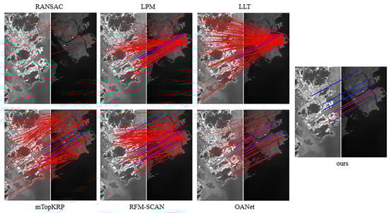
Figure 10.
Comparison of seven feature matching methods. The points connected by line segments are the inliers. Blue indicates true positives, and red indicates false positives.
Table 2.
Feature matching results of the seven methods for the OHS data. The registration results are evaluated using the four indicators: time, precision, recall, and F-score. The best results are marked in bold.
4.3.2. Interband Registration
Table 3 shows the interband registration results of the seven methods. Since the five points extracted by RANSAC in feature matching are all outliers, the three indicators all get the relatively worst results. In addition, the proposed method achieves the best results in interband registration due to the highest accuracy in the feature matching process. The other methods have relatively large registration errors because of their low precision.
Table 3.
Interband registration results of the seven methods for the OHS data. The RMSE, MAE, and MEE are used for the evaluation, and the best results are marked in bold.
4.4. Supplementary Experiment
Since the interband registration only has translational transformation, in order to show the robustness of our descriptor to various scenarios, we added related supplementary experiments. As shown in Figure 11, (a) is the 15th band of OHS image; (b) is the image of OHS 8th band image after artificial rotation and scaling transformation are added; (d) is the image of OHS 8th band image after artificially adding salt and pepper noise. Experiments have shown that we have achieved good registration results, proving that our four-dimensional descriptor is highly robust to rotation and scaling transformations, and at the same time is not sensitive to noise.
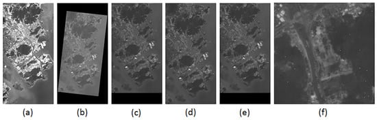
Figure 11.
Rotation, scaling, and noise experiment of OHS data. (a) is the target image; (b) is the original image with artificial rotation and scaling transformation, (c) is the registration result of (b); (d) is the target image with artificial noise; (e) is the registration result of (d); (f) is the detail display of (d) adding noise.
4.5. Discussion
As a highly practical method for interband registration of hyperspectral images, the main advantages of this method are as follows.
Robustness: The method is robust, even when the outlier rate exceeds 90%. Similar methods are highly sensitive to a high outlier rate, leading to divergence or convergence to a local minimum during the iteration. Our method has high registration accuracy for data with a high outlier rate due to image blur or multi-modal registration.
Efficiency: The algorithm has a time complexity of only O(N) and can match thousands of feature points within 0.5 s. This advantage is attributed to the efficiency of the k-means algorithm and the dimensionality reduction strategy.
High accuracy: The proposed method achieved the best matching performance and registration accuracy in the hyperspectral images experiment. The reasons are the use of the four-dimensional descriptors based on the data characteristics and the adaptive search for the most suitable k in the iterative process.
The limitations of this method are twofold.
The initial k value: The proposed method is sensitive to the initial value of k in the first iteration. The automatic extract of the k value is slightly inferior to manual extraction with regard to the registration results.
Non-rigid transformation registration ability is low: if two images have non-rigid transformations, there are many different local transformations in the images, which puts forward higher requirements on the number of inliers. After the iterative clustering is completed, often only the type of feature points with the highest degree of similarity are obtained, so it is difficult to match features in non-rigid transformations.
5. Conclusions
In this article, we proposed a feature matching method based on iterative clustering for interband registration of hyperspectral images. We developed four-dimensional descriptors based on the geometric, radiometric, and feature properties of the data to deal with blurred images and the multi-modal characteristics of some bands. After using principal component analysis, we eliminated mismatches through iterative clustering and complete registration using TPS interpolation. For feature matching, we designed an adaptive strategy suitable to the hyperspectral images. From our four kinds of experimental results, compared with several classic or latest methods, our method has a huge advantage in accuracy and is robust to a variety of remote sensing scenes, remote sensing data, and transformation types. Besides, the algorithm performed matching of thousands of feature points in about 0.5 s, laying a solid foundation to implement on-board processing in the future.
Author Contributions
S.W. carried out the empirical studies, the literature review, and drafted the manuscript; R.Z., Q.L., K.Q., Q.Z. helped to draft and review the manuscript, and communicated with the editor of the journal. All authors have read and agreed to the published version of the manuscript.
Funding
This research is supported by the National Natural Science Foundation of China: [Grant Number 42071444].
Institutional Review Board Statement
Not applicable.
Informed Consent Statement
Not applicable.
Data Availability Statement
Not applicable.
Acknowledgments
The author thanks Zhuhai Orbita Aerospace Technology Co., Ltd. Zhuhai, Guangdong Province for its data support.
Conflicts of Interest
The authors declare no conflict of interest.
References
- Ma, Y. Fusion of high spatial resolution and high spectral resolution remote sensing images. Infrared 2003, 000(010), 11–16. [Google Scholar]
- Lowe, D. Distinctive Image Features from Scale-Invariant Keypoints. Int. J. Comput. Vis. 2004, 20, 91–110. [Google Scholar] [CrossRef]
- Bay, H.; Ess, A.; Tuytelaars, T.; Gool, L.V. Speeded-Up Robust Features (SURF). Comput. Vis. Image Underst. 2008, 110, 346–359. [Google Scholar] [CrossRef]
- Rublee, E.; Rabaud, V.; Konolige, K.; Bradski, G. ORB: An efficient alternative to SIFT or SURF. In Proceedings of the 2011 International Conference on Computer Vision, Barcelona, Spain, 6–13 November 2011. [Google Scholar]
- Dalal, N.; Triggs, B. Histograms of Oriented Gradients for Human Detection. In Proceedings of the 2005 IEEE Computer Society Conference on Computer Vision and Pattern Recognition (CVPR’05), San Diego, CA, USA, 20–25 June 2005. [Google Scholar]
- Ye, Y.; Bruzzone, L.; Shan, J.; Bovolo, F.; Zhu, Q. Fast and Robust Matching for Multimodal Remote Sensing Image Registration. IEEE Trans. Geoence Remote Sens. 2019, 57, 9059–9070. [Google Scholar] [CrossRef]
- Ye, Y.; Shen, L. Hopc: A novel similarity metric based on geometric structural properties for multi-modal remote sensing image matching. ISPRS Ann. Photogramm. Remote Sens. Spat. Inf. 2016, 3, 9. [Google Scholar] [CrossRef]
- Fischler, M.A. Random sample consensus: A paradigm for model fitting with applications to image analysis and automated cartography. Read. Comput. Vis. 1987, 726–740. [Google Scholar] [CrossRef]
- Torr, P.; Zisserman, A. MLESAC: A New Robust Estimator with Application to Estimating Image Geometry. Comput. Vis. Image Underst. 2000, 78, 138–156. [Google Scholar] [CrossRef]
- Ni, K.; Jin, H.; Dellaert, F. GroupSAC: Efficient consensus in the presence of groupings. In Proceedings of the 2009 IEEE 12th International Conference on Computer Vision, Kyoto, Japan, 29 September–2 October 2009. [Google Scholar]
- Chum, O.; Matas, J.; Kittler, J. Locally Optimized RANSAC. In Lecture Notes in Computer Science; Springer: Berlin/Heidelberg, Germany, 2003. [Google Scholar]
- Lebeda, K.; Matas, J.; Chum, O. Fixing Locally Optimized RANSAC—Full Experimental Evaluation. In Proceedings of the British Machine Vision Conference, Surrey, UK, 3–7 September 2012. [Google Scholar]
- Chum, O.; Matas, J. Optimal randomized RANSAC. IEEE Trans. Pattern Anal. Mach. Intell. 2008, 30, 1472–1482. [Google Scholar] [CrossRef]
- Parra Bustos, A.; Chin, T.J. Guaranteed Outlier Removal for Point Cloud Registration with Correspondences. IEEE Trans. Pattern Anal. Mach. Intell. 2017, 40, 2868–2882. [Google Scholar] [CrossRef]
- Jiang, X.; Ma, J.; Fan, A.; Xu, H.; Tian, X. Robust Feature Matching for Remote Sensing Image Registration via Linear Adaptive Filtering. IEEE Trans. Geoence Remote Sens. 2020, 1–15. [Google Scholar] [CrossRef]
- Ma, J.; Zhao, J.; Guo, H.; Jiang, J.; Gao, X. Locality Preserving Matching. Int. J. Comput. Vis. 2019, 127, 512–531. [Google Scholar] [CrossRef]
- Jiang, X.; Jiang, J.; Fan, A.; Wang, Z.; Ma, J. Multiscale Locality and Rank Preservation for Robust Feature Matching of Remote Sensing Images. IEEE Trans. Geoence Remote Sens. 2019, 57, 6462–6472. [Google Scholar] [CrossRef]
- Ma, J.; Zhou, H.; Zhao, J.; Gao, Y.; Jiang, J.; Tian, J. Robust Feature Matching for Remote Sensing Image Registration via Locally Linear Transforming. IEEE Trans. Geoence Remote Sens. 2015, 53, 6469–6481. [Google Scholar] [CrossRef]
- Ma, J.; Jiang, X.; Jiang, J.; Guo, X. Robust Feature Matching Using Spatial Clustering With Heavy Outliers. IEEE Trans. Image Process. 2019, 29, 736–746. [Google Scholar]
- Ester, M.; Kriegel, H.P.; Sander, J.; Xu, X. A Density-Based Algorithm for Discovering Clusters in Large Spatial Databases with Noise. Kdd 1996, 96, 226–231. [Google Scholar]
- Yi, K.; Trulls, E.; Ono, Y.; Lepetit, V.; Salzmann, M.; Fua, P. Learning to Find Good Correspondences. In Proceedings of the IEEE Conference on Computer Vision and Pattern Recognition (CVPR), Salt Lake City, UT, USA, 18–22 June 2018. [Google Scholar]
- Zhao, C.; Cao, Z.; Li, C.; Li, X.; Yang, J. NM-Net: Mining Reliable Neighbors for Robust Feature Correspondences. In Proceedings of the IEEE/CVF Conference on Computer Vision and Pattern Recognition (CVPR), Long Beach, CA, USA, 16–20 June 2019. [Google Scholar]
- Wang, S.; Quan, D.; Liang, X.; Ning, M.; Guo, Y.; Jiao, L. A deep learning framework for remote sensing image registration. ISPRS J. Photogramm. Remote Sens. 2018, 145, 148–164. [Google Scholar] [CrossRef]
- Zhang, J.; Sun, D.; Luo, Z.; Yao, A.; Zhou, L.; Shen, T.; Chen, Y.; Liao, H.; Quan, L. Learning Two-View Correspondences and Geometry Using Order-Aware Network. In Proceedings of the IEEE/CVF International Conference on Computer Vision (ICCV), Seoul, Korea, 27 October–2 November 2019. [Google Scholar]
- Marin, M.; Moonen, L.; Deursen, A.V. Seventh IEEE International Working Conference on Source Code Analysis and Manipulation-Title. In Proceedings of the IEEE Seventh IEEE International Working Conference on Source Code Analysis and Manipulation (SCAM 2007), Paris, France, 30 September–1 October 2007; pp. 101–110. [Google Scholar]
- Bellman, R. Dynamic Programming. Science 1966, 153, 34–37. [Google Scholar] [CrossRef] [PubMed]
- Hinneburg, A.; Aggarwal, C.C.; Keim, D.A. What Is the Nearest Neighbor in High Dimensional Spaces? In Proceedings of the 26th Internat. Conference on Very Large Databases, Cairo, Egypt, 10–14 September 2000. [Google Scholar]
- MacQueen, J. Some methods for classification and analysis of multivariate observations. Berkeley Symp. Math. Stat. Probab. 1967, 5.1, 281–297. [Google Scholar]
- Huang, Z. Extensions to the k-Means Algorithm for Clustering Large Data Sets with Categorical Values. Data Min. Knowl. Discov. 1998, 2, 283–304. [Google Scholar] [CrossRef]
- George Karypis, E.A. CHAMELEON: A Hierarchical Clustering Algorithm Using Dynamic Modeling. Computer 2008, 32, 68–75. [Google Scholar] [CrossRef]
- Dempster, A.P. Maximum likelihood from incomplete data via the EM algorithm. J. R. Stat. Soc. 1977, 39, 1–22. [Google Scholar]
- Kohone, T. Self Organizing Feature Maps; Springer: Berlin/Heidelberg, Germany, 1988. [Google Scholar]
- Peter, R.J. Silhouettes: A graphical aid to the interpretation and validation of cluster analysis. J. Comput. Appl. Math. 1999, 20, 53–65. [Google Scholar]
- Calinski, T.; Harabasz, J. A dendrite method for cluster analysis. Commun. Stat. 1974, 3, 1–27. [Google Scholar]
- Bookstein, F.L. Principal warps: Thin-plate splines and the decomposition of deformations. IEEE Trans. Pattern Anal. Mach. Intell. 2002, 6, 567–585. [Google Scholar] [CrossRef]
- Li, Q.; Zhong, R.; Wang, Y. A Method for the Destriping of an Orbita Hyperspectral Image with Adaptive Moment Matching and Unidirectional Total Variation. Remote. Sens. 2019, 11, 2098. [Google Scholar] [CrossRef]


Publisher’s Note: MDPI stays neutral with regard to jurisdictional claims in published maps and institutional affiliations. |
© 2021 by the authors. Licensee MDPI, Basel, Switzerland. This article is an open access article distributed under the terms and conditions of the Creative Commons Attribution (CC BY) license (https://creativecommons.org/licenses/by/4.0/).