Abstract
The paper gives an overview of a ground penetrating radar (GPR) experiment to survey debonding areas within pavement structure during accelerated pavement tests (APT) conducted on the university Gustave Eiffel’s fatigue carrousel. Thirteen artificial defect sections composed of three types of defects (Tack-free, Geotextile, and Sand-based) were embedded during the construction phase between the top and the base layers. The data were collected in two stages covering the entire life cycle of the pavement structure using four GPR systems: An air-coupled ultra-wideband GPR (SF-GPR), two wideband 2D ground coupled GPRs (a SIR-4000 with a 1.5 GHz antenna and a 2.6 GHz-StructureScan from GSSI manufacturer), and a wideband 3D GPR (from 3D-radar manufacturer). The first stage of the experiments took place in 2012–2013 and lasted up to 300 K loadings. During this stage, the pavement structure presented no clear degradation. The second stage of experiments was conducted in 2019 and continued until the pavement surface demonstrated a strong degradation, which was observed at 800 K loadings. At the end of the GPR experiments, several trenches were cut at various sections to get the ground truth of the pavement structure. Finally, the GPR data are processed using the conventional amplitude ratio test to study the evolution of the echoes coming from the debonded areas.
1. Introduction
Evaluation of road structures is of major importance to maintain their durability and extend their lifetime [1]. Damages due to heavy traffic may result from a weak or defective bonding between asphalt layers [2,3]. So, early detection of delamination in asphalt pavement is a challenge for appropriate maintenance or rehabilitation strategy. In this context, ground-penetrating radar (GPR) is part of efficient non-destructive testing (NDT) for the evaluation of road structures, for thicknesses estimation, and in particular for crack and debonding damages [4,5,6,7,8].
One project of the second Strategic Highway Research Program (SHRP-2) from the US has focused on asphalt pavement delamination. The results of research and experiments are gathered in several reports, dedicated to modeling and experimental tests performed on test and real sections by different NDT including radar systems from three manufacturers [9,10]. Among their conclusions, confirming those from [4,5,6,7,8], they state that GPR can detect moderate to severe delamination as interpretation of coherent anomalies at specific depths. Moreover, this detection is facilitated when water is present and induces damages (stripping) even if not particularly sensitive to severity.
In asphalt pavements, if two layers of HMA are well bonded, the only detectable effect in the GPR signal would be caused by the difference in dielectric properties between the two layers. Amplitude of such an echo is normally low as asphalt materials constituting the bond layers are very similar (coming from the same asphalt plant that uses the same bitumen and local aggregate type). When delamination occurs, the damage and water infiltration at the debonded area can produce stronger anomalous reflections, which can potentially be detected with GPR. Nevertheless, a limitation of debonding and crack detection can occur while radar wavelengths remain much larger than the thin layer of degradation at the interface of two bituminous layers.
The RILEM committee (TC 241-MCD) has conducted a state-of-the-art review for a fundamental understanding on the mechanism of cracking and debonding in asphalt and composite pavements [11]. It highlights in particular that water infiltration through cracks and other defects have significant influence on the road structure, while reducing bond strength drastically, and that temperature effects on bond behavior have to be studied more. These two points are of particular interest for accelerated pavement testing (APT). Such full-scale APT facilities enable to monitor the state of a section road all along its lifetime and be comparable to real structure under heavy traffic.
As these damages are due to traffic, a full-scale experiment, done with the pavement fatigue carrousel of the university Gustave Eiffel, has focused on the detectability of different kinds of artificial debonded areas in a pavement structure test by few GPR under a controlled traffic. The interest of such study is to monitor the test section along its service life, to create a large GPR database while studying the evolution of the test structure in terms of damage level and lateral extension, of the defects at different loading cycles.
The data collection was organized in a two-stage experiments and covers the full life-cycle of the pavement structure. During the first stage, which took place in 2012 [12], 300 K loading cycles were performed, and degradation, either in extension or evolution, was expected. Unfortunately, no visible surface degradation was observed at the end of this first stage of experiments. As a result, the ongoing experiment has prompted 6 years of several different actions, including internal and international research projects [13,14,15]. Recently, a final series of loading has occurred, with the support of three national contributions, to complete this experiment, allowing to reach an advanced level of degradation requiring repair from the point of view of the engineers managing road networks.
The article is organized as follows: Section 2 presents the accelerated pavement testing (APT), the GPR systems used during these campaigns, and the recognition of the pavement damage at the end of the experiment. Section 3 presents all the GPR results detailed and commented on per central frequency and per defect. Lastly, Section 4 describes the autopsy of the pavement structure and discusses the link between this ground truth information and GPR evaluation.
2. Design of the Accelerated Pavement Testing
2.1. The Fatigue Carrousel
The univ. Eiffel’s pavement fatigue carrousel is a full-scale road traffic simulator, with accelerated pavement testing, composed of four arms carrying the moving heavy loads (65 kN on twin wheel for this experiment) at a maximum speed of 90 km/h [12]. The test track associated with this experiment is a 25 m structure of road composed of two bituminous layers (6 cm thick wearing course and 8 cm thick base layer) over a granular sub-base.
Thirteen rectangular patches of materials (sand, geotextile, and tack-coat free interface), simulating debonded areas, were inserted at the interface between the two asphalt layers [13]. The 3 types of defect were chosen to represent at least 2 levels of interface damage that can be observed by coring during our road expertise’s or during experiments on accelerated pavement testing. The first level, simulated by I3 and I13, corresponds to a simple debonding of the layers, which separate during coring. The second level, simulated by the other insertions, corresponds to a worse defect where disintegrated materials are observed at the interface in a thin layer. Figure 1 presents the positioning of the 13 defects on the test track and Table 1 provides the detailed description of their characteristics. Designs of the accelerated pavement testing facility and the road structure test are detailed in [16,17].
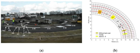
Figure 1.
Test section, (a) with the defects made during construction, (b) in the form of a site plan.

Table 1.
Characteristics of the artificial defects along the test track.
The dynamic traffic, simulated by a half-axle load for twin wheels, has been performed centered on the majority of the defects on a radius of 16 m (Figure 2a). Three hundred thousand (or 300 K) loadings were realized in 2012 [12]. As no obvious defect was detected on the structure, from a road engineer point-of-view, 500 K more loads were carried out in 2019–2020, resulting in a degradation level officially requiring repairs.
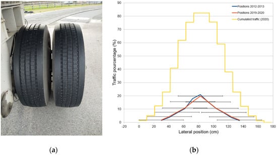
Figure 2.
(a) Dual wheels of the carrousel, (b) Traffic density vs. lateral positions of the dual wheels per 100 K loadings.
To avoid unrealistic rutting, the twin wheel was laterally displaced on 11 positions, spaced 10.5 cm apart for a 1.65 m footprint width. Figure 2b shows the location and density of lateral traffic due to lateral wandering, done in the first- and second-stage experiments, considering the 62 cm width of the twin wheel.
2.2. GPR Systems
In this section, the different GPR systems used during the two experiment stages are presented. A first group is characterized as impulse radar systems. As commercial common systems, they correspond to standards for major classical applications. Thus, three ground-coupled impulse radar were operated during this experiment, using GSSI systems; a SIR3000 device associated to a 2.6 GHz antenna during the first series in 2012, and for the 2019 series, a SIR4000 system combined with a 1.5 GHz antenna and a 2.6 GHz StructureScan (Figure 3).
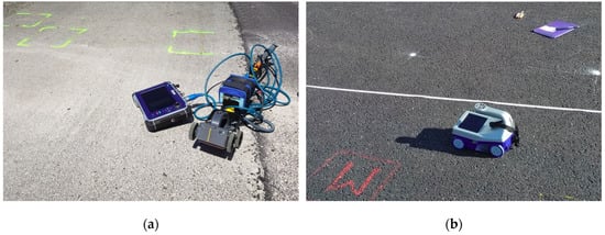
Figure 3.
Impulse radar systems: (a) SIR4000 model with a 1.5 GHz antenna, (b) 2.6 GHz StructureScan.
In the second group, stepped-frequency systems were used—an experimental one developed at university Gustave Eiffel working with an equivalent 5 GHz central frequency, and a second one, which is a commercial array system, working with an equivalent 1.5 GHz central frequency (Figure 4). In this paper, the “central frequency” of the SFR pulse is defined from the timely radar pulse signature as the inverse of the wavelength period. The latter is roughly determined from the time shift between successive zero crossing (or from the time difference between successive amplitude extrema). For the SFR parameters at hand, this practical definition provides intermediate value between the peak energy of the pulse in the Fourier domain (~3.4 GHz) and the center of the GPR bandwidth (~5.8 GHz).
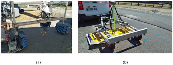
Figure 4.
(a) Univ. Eiffel’s robotic antenna-holder system associated to the stepped-frequency radar (SFR) with ultra-wide-band (UWB) antennas (surrounding blue cones are electromagnetic (EM) absorbing foams). (b) 3D-radar system during acquisition.
The univ. Eiffel’s stepped-frequency radar (SFR) relies on ultra-wide-band (UWB) radar technology. Data were collected in the frequency domain within the bandwidth 0.8 GHz–10.8 GHz using a vector network analyzer (VNA) and two air-coupled UWB Vivaldi antennas [16]. Inverse fourier transform is conventionally used to provide time domain radar data (B-scans), comparable to a 5 GHz impulse system, in the time domain.
The 3D-radar manufacturer-provided stepped-frequency 3D radar array system is composed of 21 ground-coupled antennas separated by 7.5 cm providing a sweep width of ~1.40 m. The frequency band is ranging from 40 to 3000 MHz, working with the highest range of frequency, leading, after an inverse Fourier transform, to radar data equivalent to multiple 1.5 GHz B-scan. The array system is pulled behind a vehicle and localized by an RTK centimetric global positioning system.
2.3. Acquisition and Processing Methodologies
During the experiment, radar surveys were performed at periodical loading stages. In 2012, they were focused on the largest defects, and done after the construction of the test zone, at 10 K loadings (the structure being considered as consolidated), and at around 50 K, 100 K, 200 K, 250 K, and 300 K loadings. In 2019–2020, the experiment was completed by measurements done on every defect (except the univ. Eiffel’s SFR focused on I-11, I-12, and I-13) at about 310 K, 396 K, 420 K, 500 K, 600 K, 720 K, and 800 K loadings (end of the APT). All the data were realized in the summer period, except for 720 K loading stage done end of January.
For the data collection, raw B-scans from impulse radar systems and univ. Eiffel’s SFR were taken at each loading stage, in two major directions: Transverse and longitudinal at the center of the defects. Transverse profiles were performed from the inner to the outer radius of the traffic path, and the longitudinal ones in the direction I-13 to I1. For the 3D-radar system, data are presented as horizontal maps (C-scans) of the surface echoes and the ones from the interface between the two bituminous layers. From these data, longitudinal B-scans have been extracted from the center of the largest defects.
The data pre-processing differs from the radar technology. The data pre-processing steps for impulse radar is specified in Table 2. Because of the technology of acquisition, the stepped-frequency radar data are basically required to perform inverse Fourier transform to provide the temporal B-scan images (with some time gating to limit the time horizon) and some calibration steps beforehand to take into account the antenna response in free space.
Table 2.
Pre-processing steps performed on 2.6 GHz GSSI data.
Figure 5a,b compares the pre-processed B-scan data obtained by the 2.6 GHz impulse radar and the 5 GHz SFR radar on I-11 (sand) at 720 K loadings. For the sake of clarity, the vertical time scales have been harmonized. The surface echo at the top shows the strongest amplitude, and it is called direct wave (DW) for both data types. The second strongest echo is the reflected wave (RW) from the sand-based debonded interface. The reflected echo from the healthy area shows a weaker amplitude at roughly the same time-depth.
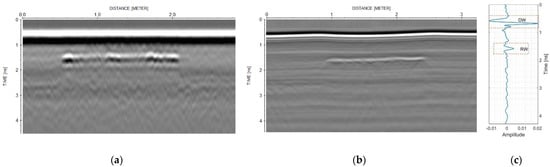
Figure 5.
Examples of B-scans performed at 720 K loadings on the defect I11 (sand) by (a) the ground-coupled 2.6 GHz impulse system and (b) the air-coupled 5 GHz stepped-frequency system. (c) A-scan extracted from Figure 5b on the defect and showing the direct wave (DW) and the reflected wave (RW).
The next step in detection debonding requires to compute, for each A-scan, the conventional amplitude ratio test (ART) as the ratio between the reflected wave (RW) and the direct wave (DW), namely, ART = RW/DW [15,18]. Then, the data processing basically consists of automatically picking the maximum (or minimum) amplitude of the two latter echoes with some existing commercial radar software. In terms of pavement monitoring, any debonding provides additional echoes, which mostly interact constructively with each other, resulting in an increased signal amplitude of the reflected signal (RW) compared to the one of the healthy zone. The pavement monitoring then turns on analyzing the amplitude ratio variation w.r.t. traffic loading.
Moreover, as the first layer is subject to strong mechanical stresses, which are not transferred to the second layer in the zones of defects, cracking and micro-cracking appear vs. traffic much more quickly. Then, the analysis of the amplitude of the surface direct wave itself was carried out, as characterizing the first layer is also a subject of interest.
2.4. State of the Road Section at the End of the Experiment
The experiments were stopped in August 2020 after noticeable damage was seen on the pavement surface, which, in a real situation, would require some repairs. Three major types of damages occurred: Cracking, micro-cracking, and rutting. The cracks initially appeared around 500 K loading over major defect zones beginning with I13 followed by I12 and I11. Beyond this loading, the cracking and micro-cracking evolved towards an unacceptable density (see Figure 6), while the healthy zones did not present any surface cracks.
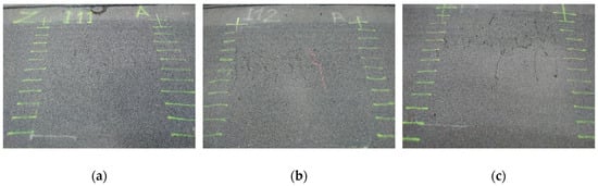
Figure 6.
Photographs of defects (a) I-11 (sand), (b) I-12 (geotextile), and (c) I-13 (tack-coat free), at stage 800 K loadings. Paints correspond to the presumed longitudinal limits of the defects.
Moreover, several cross-section profiles, done with a laser rugosimeter system, were performed showing the rutting resulting from the heavy traffic. Figure 7 presents, as an example, the cross-section profiles done in the center of I-13 and in two healthy zones (between I-11 and I-13 and between I-3 and I-4), from the inner to the outer radius of the traffic path. Measurements show rutting of above 2 cm in depth at the center of the largest defects, while it remains under 1 cm in the healthy zones.
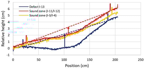
Figure 7.
Example of cross section profiles done with a laser rugosimeter after 800 K loadings, with one centered on defect I-13 and two others done on healthy zones (between defects).
3. GPR results
3.1. Introduction
This global experiment, done in two series over a period of eight years, led to the acquisition of more than 360 B-scans from impulse systems and more than 140 from stepped-frequency ones, with open-access data available in [16,17]. Processing methodology, presented in Section 2.3, has been performed on most of these data. Nevertheless, for reasons of clarity, only the major ones are presented and commented on, with the others being referenced in Appendix A, Appendix B, Appendix C and Appendix D.
A general overview is proposed thanks to GPR maps (C-scans) done by the 3D-radar system. Then, results are presented defect by defect, for the largest ones, then together for the narrowest ones.
3.2. GPR Amplitude Maps
Figure 8 presents a longitudinal profile along the center of the test section at 2.6 GHz. We note that every defect is detected (I-1 location being more ambiguous) and that defects composed of geotextile (I-4, I-9, I-10, and I-12, but not I-2) show similar echoes stronger than the others, explained by stronger dielectric contrasts. Several sensors, embedded to monitor the stress under the heavy traffic, are located in the center of I-13 and between I-12 and I-13. This is why results presented for defect I-13 in the next section will show a lack of values in the center of the data.
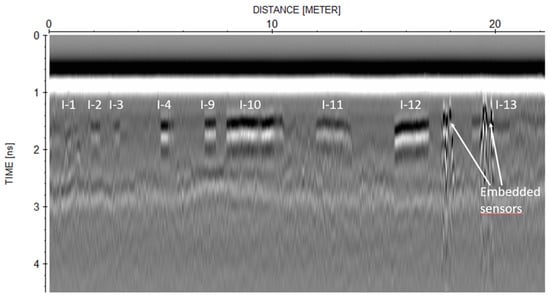
Figure 8.
Example of longitudinal B-scan performed at 2.6 GHz along the complete test section.
C-scans were performed at 396 K, 500 K, 600 K, 720 K, and 800 K loading stages, using the commercial software 3D-radar Examiner. Figure 9 shows the horizontal slices of the C-scans taken at the interface (or defect depth). These slices give an overview of the global test section and its general evolution. Most of the defects are clearly visible and their geometry well drawn. Nevertheless, the thickness and the EM state of the top layer varies due to the implementation and evolution of the asphalt layer. Therefore, they can present some bias in estimating the importance of the defects. So, it is interesting to study the amplitude of the surface direct wave (DW) and the echo at the interface of the two asphalt layers (RW), as shown in Figure 10 and Figure 11, picked in the area of I-11 to I-13.
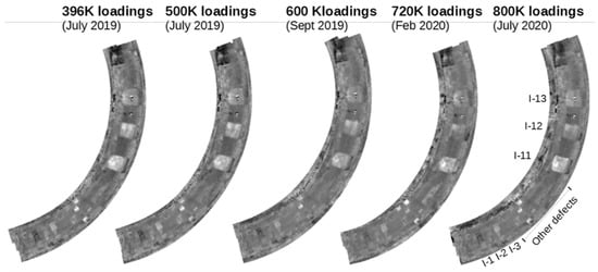
Figure 9.
RW amplitude maps of the global test zone at the defect depth, extracted from 1.5 GHz C-scans.
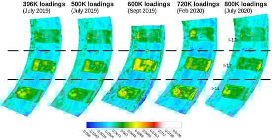
Figure 10.
Maps of the reflected echo at the defect interface extracted from C-scans in the area of I-11 to I-13 (values in Legend refer to the amplitude of the received signal).
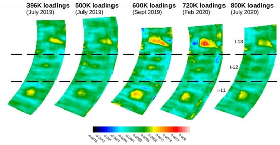
Figure 11.
Maps of the surface direct wave extracted from C-scans in the area of I-11 to I-13 (values in Legend refer to the amplitude of the received signal).
From these maps, some general observations can be made. Firstly, the heavy traffic has not induced strong lateral expansion of the defects although numerous surface cracks that appeared in the two last loading stages. The evolution of the RW amplitudes is visible on Figure 10 for increasing vs. degradation for defects I-11 and I-13 until 720 K loading stage, with defect I-12 presenting a surprisingly high amplitude level at 600 K loading stage. The last measurement stage, done in July 2020 five months after the 720 K loading one (imposed COVID confinement), shows a decreasing trend. Such a decrease of EM contrast suggests an internal moisture evaporation and possible auto-repair of the structure.
Lastly, we note that at the internal radius area the RW amplitudes are stronger. It could be due to the transverse slope towards the center of the carrousel, as shown in Figure 6, which trap the moisture at the border of the defects.
The DW maps from Figure 11 show that stronger amplitudes from the central zones of defects I-13 and I-11 (and a second-order of defect I-12) may be related to traffic. They could be attributed to greater concentration of constraints inducing visible cracking in Figure 6, and so, an increase of surface porosity and a lower permittivity. Another possibility could be the effect of the rutting (several millimeters) on the direct wave due to loss of contact of the antenna array on the ground.
Complementary measurements done by bi-static systems on the centers of the defects make comparisons possible.
3.3. Study of the Largest Defects I-11 to I-13
The processed maps from the C-scans show variations in the DW, and thus, suggest an evolution of the state of the pavement layer. This also reinforces the use of amplitude ratio approach to process all the B-scans. The approach further enables to estimate the evolution, the degradation of RW above defects, and possibly compare different central frequency results.
The following sub-sections detail the results per central frequency, from 2.6 GHz considered as a commonly used central frequency for this application, to 1.5 and 5 GHz. Appendix A gives some B-scans examples, done on the I-12 defect, for every central frequency.
3.3.1. Study of Defects I-11 to I-13 at 2.6 GHz
Figure 12, Figure 13 and Figure 14 gather normalized RW amplitudes, namely RW/DW as defined in Section 2.3, picked on the defects I-11, I-12 and I-13 from the 2.6 GHz data over all the loading stages.
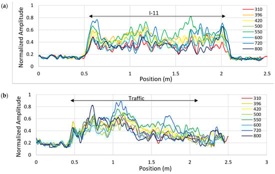
Figure 12.
2.6 GHz Norm. RW amplitudes on sand (I-11) in the (a) long. and (b) transv. direction vs. K loadings.
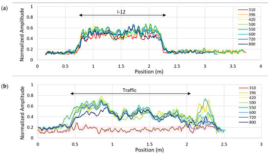
Figure 13.
2.6 GHz Norm. RW amplitudes on geotextile (I-12) in the (a) long. and (b) transv. direction vs. K loadings.
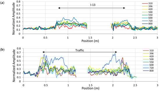
Figure 14.
2.6 GHz Norm. RW amplitudes on tack-coat free (I-13) in the (a) long. and (b) transv. direction vs. K loadings.
From these results, we can make the following observations:
- -
- In the healthy zones out and under traffic, normalized RW remains stable. Apart from a natural aging of the pavement layers, heavy traffic has had no effect on the road structure from GPR point-of-view. Moreover, due to low EM contrasts, sometimes echo picking was not easy and could lead to errors in their detection/location.
- -
- Defects are clearly visible with a high level of RW amplitude but with strong local variations. These variations could be due to local heterogeneities enhanced by internal moisture content and by the fact that GPR antennas did not pass on exactly the same path. As an example, when studying B-scans performed on the geotextile defect in Figure 13a, standard deviations in the defect area are twice to four times greater than the ones in the sound area. Geotextile and sand-based defects show stronger radar echoes due to higher EM contrasts.
- -
- Longitudinal data show stable values along the defect and no major defect expansion of it. As presented in Table 3, the amplitude threshold was fixed to 0.24. A complementary threshold value has been estimated around 0.20 and is varied depending on the evaluation by a GPR specialist (presented as manual length). Figure 15a shows that horizontal extension vs. traffic remain very low even if they show several centimetric increases at the beginning of the two periods. Moreover, some natural auto-repair during the intermediate period was observed.
Table 3. Detected characteristics of defect zones from 2.6 GHz longitudinal B-scans.
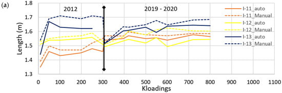
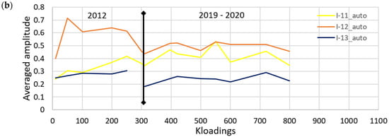 Figure 15. (a) Extensions and (b) averaged normalized amplitudes of 2.6 GHz RW on defects I-11 to I-13.
 - -
- When studying the amplitude evolution vs. traffic, we cannot make a direct link. Variations mainly come from moisture content inside the defect due to the weather conditions from the previous days, and perhaps in a second step, from variations of temperature. Table 3 summarizes this information, while giving an average value of amplitude all along the defects (Figure 15b).
- -
- Transverse data present a general trend of RW decrease while moving towards the outside of the carrousel due to the road topography promoting inward water migration and possible lateral water gradient (see Figure 7). It should be mentioned that this trend seems not to be correlated with the traffic density.
- -
- With the width of defects (2 m) being larger than the traffic path (1.65 m), outside the traffic path we do not observe any evolution of the amplitude over the defect. This comment only concerns the inner area (left parts of the Ffigures), as a tiny elevation of the pavement course, existing at the external peripherical test section, disturbs the ground-coupled GPR acquisition.
3.3.2. Study of Defects I-11 to I-13 at 1.5 GHz
Figure 16, Figure 17 and Figure 18 gather normalized RW amplitudes picked on the defects I-11, I-12, and I-13 vs. loading, from the 1.5 GHz data. Considering longitudinal results on the central axis of the traffic, we observe roughly stable levels without any general trend vs. traffic. Similar to 2.6 GHz results, transversal 1.5 GHz values present a general trend of RW decrease while moving towards the outer edge of the test track.
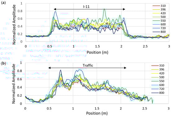
Figure 16.
1.5 GHz Norm. RW amplitudes on sand (I-11) in the (a) long. and (b) transv. direction vs. K loadings.
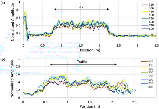
Figure 17.
1.5 GHz Norm. RW amplitudes on geotextile (I-12) in the (a) long. and (b) transv. direction vs. K loadings.
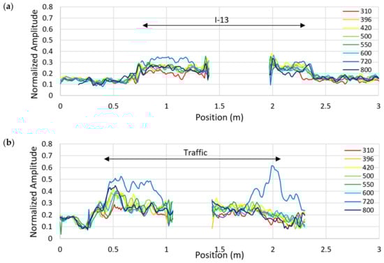
Figure 18.
1.5 GHz Norm. RW amplitudes on tack-coat free (I-13) in the (a) long. and (b) transv. direction vs. K loadings.
3.3.3. Study of Defects I-11 to I-13 at 5 GHz
When measurements are done with air-coupled antennas, the polarity of the DW and RW are inverted and the amplitude ratios present negative values. We observed, in Figure 19, Figure 20 and Figure 21, similar results to those from 2.6 GHz, with stable values for longitudinal profiles and a general trend for the transverse ones. As the acquisition length of the univ. Eiffel’s robotic antenna-holder system is limited to 1.6 m, longitudinal acquisitions were performed twice per defect. For the processing of these B-scans, they were gathered before picking, with the results being shown in Figure 19a, Figure 20a and Figure 21a. Results obtained at 5 GHz show the same trend as the 2.6 and 1.5 GHz ones.
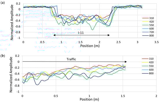
Figure 19.
5 GHz Norm. RW amplitudes on sand (I-11) in the (a) long. and (b) transv. direction vs. K loadings.
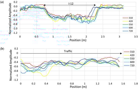
Figure 20.
5 GHz Norm. RW amplitudes on geotextile (I-12) in the (a) long. and (b) transv. direction vs. K loadings.
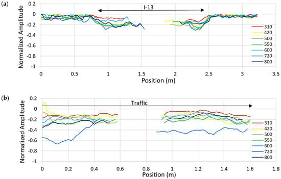
Figure 21.
5 GHz Norm. RW amplitudes on tack-coat free (I-13) in the (a) long. and (b) transv. direction vs. K loadings.
While studying normalized amplitudes, we noted that 2.6 GHz corresponded to the best central frequency for debonding detection of the pavement layer. Indeed, on the defect I-12 for example, we obtained average amplitudes of about 0.5–0.55 for 2.6 GHz, 0.45 for 1.5 GHz, and 0.5–0.55 for 5 GHz. When comparing these with the 1.5 GHz results, higher frequency, and smaller wavelength, shows better sensitivity to the very thin layer as debonding. This observation is no longer valid as, for the wavelength at 5 GHz, asphalt concrete cannot be considered as homogeneous. At such high frequencies, EM waves are scattered by the biggest aggregates (diam = 10 mm) inducing an attenuation that counterbalances their sensitivity to very-thin-layer detection.
3.4. Direct Waves in the Zone I-11 to I-13 at 2.6 GHz
Similarly, DW amplitudes are picked on the B-scans for each defect and are then normalized by averaged values of DW coming from the healthy zone, outside the traffic, from the beginning of the corresponding transverse profiles. This parametric study has been performed with 2.6 GHz data (presented in this section) and 1.5 GHz data (presented in Appendix C). Finally, the DW at 5 GHz is not included in this paper as the data are not reliable due to the variations caused by rutting.
Figure 22, Figure 23 and Figure 24 respectively present the longitudinal and transversal variation in normalized DW amplitude for 2.6 GHz data over I-11, I-12, and I-13 defects. Results show that the first layer has already suffered damage from the first series of loading in 2012, remaining from the start of the second series of loading.
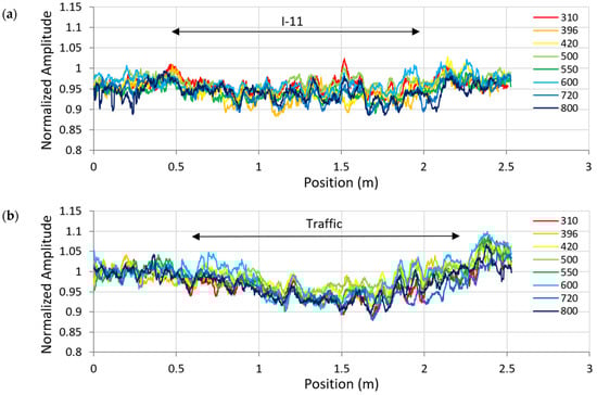
Figure 22.
2.6 GHz Norm. DW amplitudes on sand (I-11) in the (a) long. and (b) transv. direction vs. K loadings.
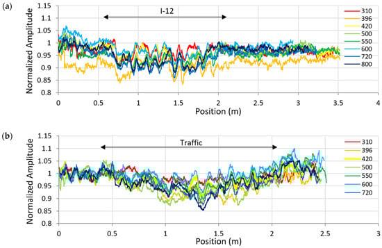
Figure 23.
2.6 GHz Norm. DW amplitudes on geotextile (I-12) in the (a) long. and (b) transv. direction vs. K loadings.
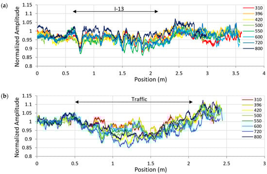
Figure 24.
2.6 GHz Normalized DW amplitudes on tack-coat free (I-13) in the (a) long. and (b) transv. direction vs. K loadings.
Longitudinal data do not show clear trend between healthy and weak zones for the defect I-11. However, detection is more visible for the two other defects (due to higher EM contrasts).
Concerning transverse data, we can note a general trend proportional to the traffic density, shown in Figure 22b, Figure 23b and Figure 24b, in a V shape with the minimum amplitude corresponding to the maximum of traffic. As the data come from ground-coupled acquisition, the decrease of the normalized amplitudes could be associated with an increase of the relative permittivity of the first asphalt, which narrows the radiation pattern and thus decreases the DW amplitude. This finding, when associated with the increase of cracks in the first layer, can be interpreted as an increase of moisture content trapped in this opened porosity.
3.5. Study of Defects I-1 to I-3
Defects I-1 to I-3 correspond respectively to defects I-11 to I-13 with a narrow width of 50 cm. Measurements were only done at 1.5 and 2.6 GHz, with GSSI systems during the second stages of experiment. Only 2.6 GHz data are processed and presented in this section as the 1.5 GHz and 2.6 GHz data are very similar. From Figure 25, Figure 26, Figure 27 and Figure 28, we note that the narrowness of the defects induces different behavior under traffic than I-11 to I-13. The amplitudes do not appear to be stable along the longitudinal traces of I1 to I3. Additionally, no V-shaped variation in trends is seen for the transversal results over the largest defects. This phenomenon could be explained by the loading transfer in the asphalt partially supported by the healthy borders, and then not damaging the surveyed interface.
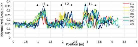
Figure 25.
2.6 GHz Normalized RW amplitudes on defects I-3 to I-1, in the longitudinal direction vs. K loadings.
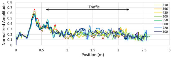
Figure 26.
2.6 GHz Normalized RW amplitudes on sand (I-1), in the transversal direction vs. K loadings.
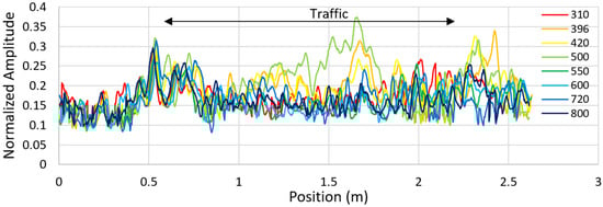
Figure 27.
2.6 GHz Normalized RW amplitudes on geotextile (I-2), in the transversal direction vs. K loadings.
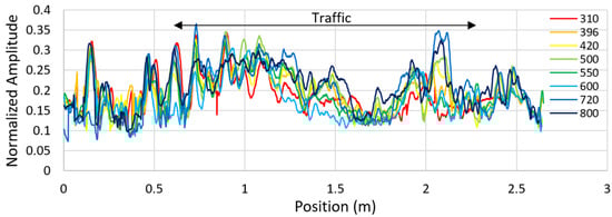
Figure 28.
2.6 GHz Normalized RW amplitudes on tack-coat free (I-3), in the transversal direction vs. K loadings.
3.6. Study of Defects I-4 to I-10
This panel of defects presents a similar interface (geotextile-based), with small or narrow dimensions and some of them being shifted from main traffic. As for defects I-1 to I-3, measurements were performed with 1.5 and 2.6 GHz GSSI systems, and only 2.6 GHz results are presented herein.
Figure 29, Figure 30, Figure 31, Figure 32, Figure 33, Figure 34, Figure 35, Figure 36, Figure 37 and Figure 38 show strong variations of normalized amplitudes from defect I-4 to I-10, depending on the loading step and the location of the defect. As a reminder, defects I-4, I-9, and I-10 are centered on the axis of the major loading traffic. Defects I-6 and I-7 are off-center, even out of traffic, and at last, defects I-5 and I-8 are out of traffic.
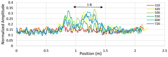
Figure 29.
2.6 GHz Normalized RW amplitudes on defect I-4, in the longitudinal direction vs. K loadings.
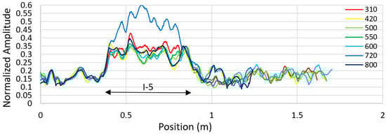
Figure 30.
2.6 GHz Normalized RW amplitudes on defect I-5, in the longitudinal direction vs. K loadings.
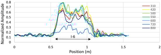
Figure 31.
2.6 GHz Normalized RW amplitudes on defect I-6, in the longitudinal direction vs. K loadings.
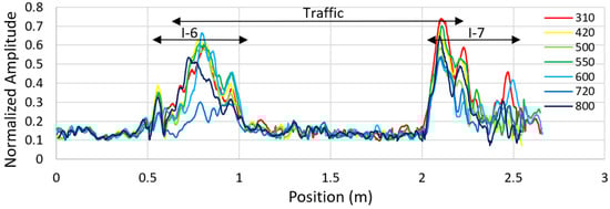
Figure 32.
2.6 GHz Normalized RW amplitudes on defects I-6 and I-7, in the transversal direction vs. K loadings.
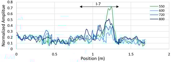
Figure 33.
2.6 GHz Normalized RW amplitudes on defect I-7, in the longitudinal direction vs. K loadings.
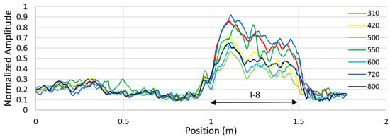
Figure 34.
2.6 GHz Normalized RW amplitudes on defect I-8, in the longitudinal direction vs. K loadings.
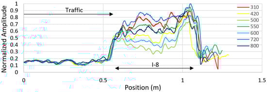
Figure 35.
2.6 GHz Normalized RW amplitudes on defect I-8, in the transversal direction vs. K loadings.
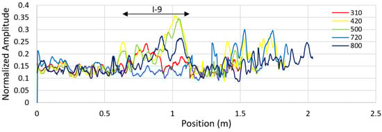
Figure 36.
2.6 GHz Normalized RW amplitudes on defect I-9, in the transversal direction vs. K loadings.
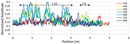
Figure 37.
2.6 GHz Normalized RW amplitudes on defects I-9 and I-10, in the longitudinal direction vs. K loadings.
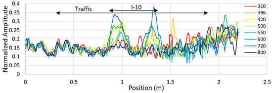
Figure 38.
2.6 GHz Normalized RW amplitudes on defect I-10, in the transversal direction vs. K loadings.
The analysis of measures done on defects I-5 and I-8 can be interesting since these areas reveal the evolution of the pavement structure without traffic function of the months and seasons. Moreover, Figure 30, Figure 31, Figure 32, Figure 33 and Figure 34, results show a variability of building. Indeed, I-5 appears to be very stable regardless of the traffic step and the period of acquisition (the exception being the 720 K loading step, the only one done in winter), while I-8 shows strong variations, which may be due to variation of water ingress.
Defects I-4, I-9, and I-10, located on the center of the traffic zone, present amplitude values roughly two times lower than the value obtained from defect I-12, with some punctual zones in which amplitude values exceed just the average of neighboring healthy areas. These strong variations of EM contrasts suggest variation of tack coat gluing, inducing possible water ingress.
Most surprising is the shape of I-10 results (Figure 38) showing detection only on the borders of the defect. Amplitudes are growing vs. traffic during the summer 2019 (from 310 K to 550 K loadings) and a slow decrease at 600 K loading step. For these last measurements, the explanation could come from the fact that the heavy traffic, going towards 600 K loadings, was realized several weeks before GPR measurements, letting the structure auto-repair with the high temperatures. We find a similar situation for the 800 K loading step: Low radar amplitudes, measurements done at the end of May, and traffic cycles done numerous weeks before. The exception comes from the 720 K loading steps, as GPR measurements were performed in winter (January 2020) during a cold and rainy period, and showing strong EM contrasts may be due to water ingress. This analysis, done on defect I-10, is representative of almost other defects.
4. Autopsy of the Road Section
4.1. Extraction of Transversal Blocks
At the end of the loading series and GPR experiments, several trench cores were sampled to get a ground truth of the damaged structure, and first of all, the real thickness of the defects and their lateral length. Six trenches have been realized in the area of the largest defects. Four transverse trenches were located at the center of defects I-10, I-11, I-12, and I-13, at the level of the GPR profiles, and dimensions of approximately as follows: 1.30 × 0.25 × 0.15 m (Figure 39). One transverse trench was done between defects I-11 and I-12 to obtain information of the traffic effect on a healthy zone. The last one was sawn longitudinally from the center of I-12 towards I-13, 1.2 m long.
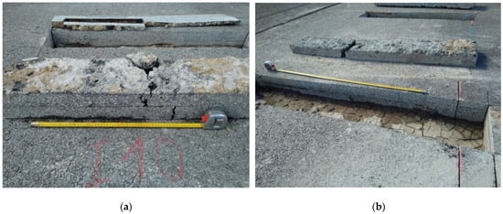
Figure 39.
Transverse trenches and corresponding asphalt slabs of (a) defect I-10 and (b) defects I-12.
During the extraction of the blocks, all but the healthy one broke, as shown in Figure 39a. From the perspective of road experts, this was due to weakness of the top layer from the defective zones, presenting numerous vertical micro-cracks on the side (some of them being attributed to the extraction).
Going into detail (Figure 40), the findings are as follows:
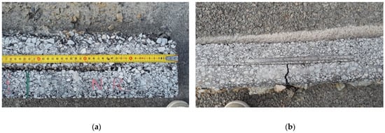
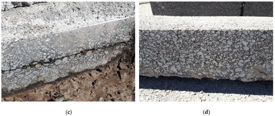
Figure 40.
Details of defects visible on the side of asphalt slabs, based on (a) sand (I-11), (b) geotextile (I-10), (c) tack-coat free (I-13), and (d) healthy zone.
- -
- The geotextile-based defect presents no clear degradation. The geotextile is about 5 mm thick and remains glued to the layer 1. When it is debonded to layer 2, we cannot see its lateral extension.
- -
- Concerning the sand-based defect, a layer of void is visible due to sawing under water, which carried away the sand. The apparent thickness of this debonding is about 3 mm, with a maximum of 11 mm near the inner radius and a minimum around 1.2 mm seen near the center of the traffic. Moreover, it seems that no aggregates were loosened from one of the two asphalt layers.
- -
- The tack-free-based defect presents a narrow debonding (visible by wetting in Figure 40c) all along the defect of sub-millimeter to millimeter thickness, but no loose aggregates.
To conclude, the extracted blocks and the trenches have shown no loosing of material from asphalt layers, but only micro-cracks, mainly vertically oriented.
4.2. Estimation of Void Content and Relative Permittivity
The estimation of void content has been performed on layer 1 of the trenched block, extracted over I-10. It was then tested under gamma radiation in the laboratory several weeks after its extraction. Gammadensimetry, a semi-destructive radiation method (Figure 41a), is viewed as a reliable laboratory testing method and considered as a reference in the field of the bulk density variation measurement [19].
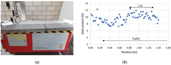
Figure 41.
(a) Gammadensimetric acquisition on asphalt layer, (b) void content estimation vs. of lateral location.
Measurements were performed on six parallel lines of 1.4 m long. While considering an average bulk density of the asphalt, a void content value is calculated every 2 cm. As the gamma ray is very narrow (>10 mm), an average is done so that values are representative of the mixing vs. location of the traffic (Figure 41b).
Data show that the asphalt presents higher void content (~10.5%) above the defect than in healthy zone under traffic (~8.7%), which can be explained by higher density of micro-cracks.
In parallel, two actions were performed to estimate the permittivity of the asphalt layer 1 along the transversal direction. First, travel time Δt in layer 1 was extracted from the automatic time picking of the 2.6 GHz amplitude Bscan done on I-10 after the 800 K loading step, taking account the ground-coupled bistatic mode (offset X) of acquisition (Figure 42a). While knowing the thickness of the layer 1, this approach is complementary to [20] studying the GPR amplitude vs. compaction.
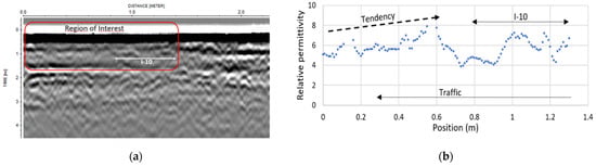
Figure 42.
(a) 2.6-GHz transversal profile done on defect I-10 at 800 K loadings. (b) Estimation of the relative permittivity of the asphalt layer 1.
Second, 12 Mpx images were taken on the side of the asphalt slab. An operator manually calibrated the images in size and accurately measured the thickness D of layer 1 every 1 cm along the entire length.
From this information, the relative permittivity of the asphalt layer can be calculated as presented in Figure 42b, using the following equation where c is the velocity in the air:
We note an increase of permittivity while going from the inner area toward the center of traffic in the first 0.6 m. Then, picking is biased by the defect I-10. This result is compatible with the ones obtained from 2.6-GHz DW in Figure 22, Figure 23 and Figure 24, as the increase of permittivity reduces the radiation pattern and then the DW amplitude. A possible interpretation is an increase of porosity (or micro-cracking) in which humidity has penetrated and is kept by capillary effect.
The decrease of relative permittivity of the asphalt slab from gammadensimetry results, being correlated to an increase of porosity or micro-cracking, is explained by an indoor natural drying before measurements.
These results show an opposite tendency to the ones observed on the measurements of the 1.5 GHz Stepped-frequency array system (Figure 11). A possible explanation could come from the fact that the antennas, inserted in a wide plastic box, lie at a small height from the asphalt layer. This could induce a merge of an aerial direct wave and with the direct wave in the surveyed medium, and then an increase of amplitude as the permittivity of the layer decreases.
5. Conclusions
A major GPR experiment was performed on a full-scale accelerated pavement testing at the university Gustave Eiffel, on a section presenting three artificial defects of bonding (tack-free, geotextile, and sand-based). Measurements were done periodically with several GPR systems all along the life-cycle of the road structure in two stages: 300 K loadings in 2012–2013 and 500 K loadings in 2019–2020 leading to a structure considered as strongly degraded.
Four GPR systems were tested, mainly during the second stage of experiment from 1.5 to 5 GHz central frequency. More than 500 GPR profiles were acquired, most of them being processed for this paper. Data processing was focused on the amplitude analysis (amplitude ratio test) of the reflected waves at the interface of the defects and on the direct waves.
The major results are the following:
- -
- Defects are detected almost all the time (with exceptions), due to sufficient dielectric contrasts. The geotextile defect presents the strongest EM contrast followed by the sand-based defect, with the tack-free defect being nevertheless detectable.
- -
- Debondings did not show lateral expansions during the life-cycle of the tested structure.
- -
- Variations of normalized reflected amplitude of the interface echoes did not show a reliable correlation with heavy traffic. Amplitudes appeared to be more sensitive to the meteorology (humidity, water ingress from rainy periods, temperature) and the time delay between the end of traffic step and GPR measurements. Indeed, for the first point, the appearance of micro-cracks allowed increased moisture content inside the defect due to the weather conditions from the previous days. For the second point, under high temperatures, asphalt layers with visco-elastic materials could slightly auto-repair, therefore reducing the EM contrasts.
- -
- When comparing the central frequencies for the detectability of debonding defects, considered as very thin layers, 2.6 GHz corresponds to the best frequency for debonding detection, compared to the two others. This central frequency, higher than 1.5 GHz, shows better sensitivity to very thin layer as debonding, and is not attenuated as at 5 GHz. Indeed, at such very high frequencies, EM waves are scattered by the biggest aggregates (diam. = 10 mm) inducing an attenuation that counterbalances their sensitivity to very-thin-layer detection. This phenomenon is not visible on the B-scans as the beamwidth of the air-coupled antennas induces an average on this scattering effect.
- -
- Concerning the study of GPR direct waves, we observed a general tendency showing that degradation of the surface layer is visible by GPR measurements. A general tendency of decreaing DW amplitude vs. traffic is associated with the increase in micro-cracks, and then of water content of the medium.
- -
- At last, we observe that overall, the results are similar to those from SHRP-2 [9] if we do not consider the influence of the traffic. In this report, GPR results on full-scale road sections, from five radar systems, have shown that degraded zones (no bond and stripping, similar to defects I-13 and I-11) were not always detected, with the exception of after water ingress. Moreover, the choice of time-depth slices as a detection parameter is not optimal as thicknesses of layers are not perfectly constant and thus the extracted amplitudes may not correspond to a maximum of EM contrast. This problem is removed when picking the echoes at an interface (problem solved for the 3D-radar system in 2019, see Figure 10 and Figure 11).
The database is available to the GPR community and may serve as a reference benchmark for both developing and testing the performance of various processing or monitoring purposes of debonded areas of pavement structures under full-scale controlled traffic [16,17].
Author Contributions
Conceptualization, X.D., V.B., and J.-M.S.; methodology, X.D., V.B., and J.-M.S.; software, X.D., V.B., and C.N.; validation, X.D., V.B., and J.-M.S.; formal analysis, X.D., V.B., S.S.T., C.N., and H.-Y.H.; investigation, X.D., V.B., C.N., and H.-Y.H.; resources, X.D., V.B., and J.-M.S.; data curation, X.D., V.B., and J.-M.S.; writing—original draft preparation, X.D.; writing—review and editing, X.D., V.B., and J.-M.S.; funding acquisition, X.D., V.B., and J.-M.S. All authors have read and agreed to the published version of the manuscript.
Funding
The data collection in 2019 has been supported by the French Research Agency (grant ANR-18-CE22-0020), the FEREC foundation (grant CINC-RSF), and the Ministry of Ecological and Solidarity Transition (grant MTES N° 18/402).
Institutional Review Board Statement
Not applicable.
Informed Consent Statement
Not applicable.
Data Availability Statement
Database of GPR B-scans are available at: https://doi.org/10.25578/N0RXSQ (accessed on 4 March 2021) and, https://doi.org/10.25578/MM9Q0R (accessed on 4 March 2021).
Acknowledgments
The authors would like to thank the technical staff of univ. Gustave Eiffel Carrousel (S. Trichet, T. Gouy, G. Coirier, Y. Baudry, M. L. Nguyen et J. Blanc), the one of GeoEND laboratory (O. Durand, G. Gugole and T. Devie) and J.M. Moliard from S2I laboratory. The authors also thank P.H.G. Ching for experimental help in the frame of a collaboration with Polytechnic university of Hong Kong. The first part of the data collection in 2012, has been a contribution of the RILEM technical committee TC241-MCD (“Mechanisms of cracking and debonding in asphalt and composite pavements”, www.rilem.org (accessed on 4 March 2021)) and the COST action TU1208 (“Civil engineering applications of ground-penetrating radar”).
Conflicts of Interest
The authors declare no conflict of interest. The funders, cited in the Acknowledgments section, had no role in the design of the study; in the collection, analyses, or interpretation of data; in the writing of the manuscript, or in the decision to publish the results.
Appendix A
Presentation of longitudinal B-scans performed at about 396 K and 720 K loadings on the defect I-12.

Figure A1.
1.5 GHz impulse B-scans performed on geotextile (I-12) at (a) 396 K and (b) 720 K loadings.
Figure A1.
1.5 GHz impulse B-scans performed on geotextile (I-12) at (a) 396 K and (b) 720 K loadings.


Figure A2.
1.5 GHz stepped-frequency B-scans performed on geotextile (I-12) at (a) 396 K and (b) 720 K loadings.
Figure A2.
1.5 GHz stepped-frequency B-scans performed on geotextile (I-12) at (a) 396 K and (b) 720 K loadings.


Figure A3.
2.6 GHz impulse B-scans performed on geotextile (I-12) at (a) 396 K and (b) 720 K loadings.
Figure A3.
2.6 GHz impulse B-scans performed on geotextile (I-12) at (a) 396 K and (b) 720 K loadings.


Figure A4.
5 GHz stepped-frequency B-scans performed on geotextile (I-12) in two steps at (a,b) 420 K and (c,d) 720 K loadings.
Figure A4.
5 GHz stepped-frequency B-scans performed on geotextile (I-12) in two steps at (a,b) 420 K and (c,d) 720 K loadings.

Appendix B
Presentation of normalized RW amplitudes of 2.6 GHz GPR profiles done on defects I-11 to I-13 during the 2012 series.

Figure A5.
2.6 GHz normalized RW amplitudes on sand (I-11) in the longitudinal direction vs. K loadings.
Figure A5.
2.6 GHz normalized RW amplitudes on sand (I-11) in the longitudinal direction vs. K loadings.


Figure A6.
2.6 GHz normalized RW amplitudes on geotextile (I-12) in the longitudinal direction vs. K loadings.
Figure A6.
2.6 GHz normalized RW amplitudes on geotextile (I-12) in the longitudinal direction vs. K loadings.


Figure A7.
2.6 GHz normalized RW amplitudes on tack-coat free (I-13) in the long. direction vs. K loadings.
Figure A7.
2.6 GHz normalized RW amplitudes on tack-coat free (I-13) in the long. direction vs. K loadings.

Appendix C
Presentation of normalized DW amplitudes of 1.5 GHz GPR profiles done on defects I-11 to I-13 during the 2019–2020 series.

Figure A8.
1.5 GHz Norm. DW amplitudes on sand (I-11) in the (a) long. and (b) transv. direction vs. K loadings.
Figure A8.
1.5 GHz Norm. DW amplitudes on sand (I-11) in the (a) long. and (b) transv. direction vs. K loadings.


Figure A9.
1.5 GHz Norm. DW amplitudes on geotextile (I-12) in the (a) long. and (b) transv. direction vs. K loadings.
Figure A9.
1.5 GHz Norm. DW amplitudes on geotextile (I-12) in the (a) long. and (b) transv. direction vs. K loadings.


Figure A10.
1.5 GHz Norm. DW amplitudes on tack-coat free (I-13) in the (a) long. and (b) transverse direction vs. K loadings.
Figure A10.
1.5 GHz Norm. DW amplitudes on tack-coat free (I-13) in the (a) long. and (b) transverse direction vs. K loadings.

Appendix D
Presentation of DW amplitudes of 2.6 GHz GPR profiles done on defects I-11 to I-13 during the 2012 series.

Figure A11.
2.6 GHz DW amplitudes on sand (I-11) in the longitudinal direction vs. K loadings.
Figure A11.
2.6 GHz DW amplitudes on sand (I-11) in the longitudinal direction vs. K loadings.


Figure A12.
2.6 GHz DW amplitudes on geotextile (I-12) in the longitudinal direction vs. K loadings.
Figure A12.
2.6 GHz DW amplitudes on geotextile (I-12) in the longitudinal direction vs. K loadings.


Figure A13.
2.6 GHz DW amplitudes on tack-coat free (I-13) in the longitudinal direction vs. K loadings.
Figure A13.
2.6 GHz DW amplitudes on tack-coat free (I-13) in the longitudinal direction vs. K loadings.

References
- Baltazart, V.; Moliard, J.-M.; Amhaz, R.; Cottineau, L.-M.; Wright, A.; Wrigh, D.; Jethwa, M. Automatic Crack Detection on Pavement Images for Monitoring Road Surface Conditions—Some Results from the Collaborative FP7 TRIMM Project. In 8th RILEM International Conference on Mechanisms of Cracking and Debonding in Pavements; Springer: Dordrecht, The Netherlands, 2016; Volume 13, pp. 719–724. [Google Scholar] [CrossRef]
- Kruncheva, M.R.; Collop, A.C.; Thrn, N.H. Effect of bond condition on flexible pavement performance. J. Transp. Eng. 2005, 131, 880–888. [Google Scholar] [CrossRef]
- Gharbi, M.; Nguyen, M.L.; Chabot, A. Characterization of debonding at the interface between layers of heterogeneous materials coming from roads. In Proceedings of the Congrès Francçais de Mécanique, Lille, France, 28 August–1 September 2017. [Google Scholar]
- Saarenketo, T.; Scullion, T. Road evaluation with ground penetrating radar. J. Appl Geophys. 2000, 43, 119–139. [Google Scholar] [CrossRef]
- Plati, C.; Georgouli, K.; Loizos, A. A Review of NDT assessment of road pavements using GPR. RILEM Books 2012, 6, 855–860. [Google Scholar]
- Solla, M.; Lagüela, S.; Gonzalez, H.; Arias, P. Approach to identify cracking in asphalt pavement using GPR and infrared thermographic methods: Preliminary findings. NDT E Int. 2014, 62, 55–65. [Google Scholar]
- Marecos, V.; Solla, M.; Fontul, S.; Antunes, V. Assessing the pavement subgrade by combining different non-destructive methods. J. Constr. Build. Mat. 2017, 135, 76–85. [Google Scholar] [CrossRef]
- Lai, W.L.; Dérobert, X.; Annan, A.P. A review of ground penetrating radar application in civil engineering: A 30-year journey from locating, testing and evaluation to imaging and diagnosis. NDT E Int. 2018, 96, 58–78. [Google Scholar]
- Nondestructive Testing to Identify Delaminations between HMA Layers; SHRP-2 report S2-R06D-RW-3; Transportation Research Board: Washington, DC, USA, 2013; Volume 3, p. 146.
- Nondestructive Testing to Identify Delaminations between HMA Layers; SHRP-2 report S2-R06D-RW-4; Transportation Research Board: Washington, DC, USA, 2013; Volume 4, p. 158.
- Buttlar, W.; Chabot, A.; Dave, E.V.; Petit, C.; Tebaldi, G. RILEM State Art Reports. In Mechanisms of Cracking and Debonding in Asphalt and Composite Pavements; Springer: Cham, Germany, 2018; Volume 28, p. 237. [Google Scholar]
- Simonin, J.M.; Baltazart, V.; Hornych, P.; Kerzrého, J.P.; Dérobert, X.; Trichet, T.; Durand, O.; Alexandre, J.; Joubert, A. Detection of debonding and vertical cracks with ND techniques during accelerated tests. In Proceedings of the Accelerated Pavt Testing (APT) Conference, Davis, CA, USA, 19–21 September 2012. [Google Scholar]
- Simonin, J.M.; Hornych, P.; Baltazart, V.; Dérobert, X.; Thibaut, E.; Sala, J.; Utsi, V. Case study of detection of artificial defects in an experimental pavement structure using 3D GPR. In Proceedings of the GPR’2014 Congress, Brussels, Belgium, 30 June–4 July 2014. [Google Scholar]
- Simonin, J.M.; Baltazart, V.; Le Bastard, C.; Dérobert, X. Progress in monitoring the debonding within pavement structures during accelerated pavement testing on the Ifsttar’s fatigue carousel. In Proceedings of the 8th International RILEM Conference, Nantes, France, 7–9 June 2016. [Google Scholar]
- Todkar, S.; Le Bastard, C.; Baltazart, V.; Ihamouten, A.; Dérobert, X. Performance assessment of SVM-based classification techniques for the detection of artificial debondings within pavement structures from step-frequency A-scan radar data. NDT E Int. 2019, 107, 102128. [Google Scholar] [CrossRef]
- Derobert, X.; Baltazart, V.; Simonin, J.-M.; Durand, O.; Norgeot, C.; Doué, S. Radar database over large debonded areas. IFSTTAR 2020. [Google Scholar] [CrossRef]
- Derobert, X.; Baltazart, V.; Simonin, J.-M.; Hui, H.Y. Radar Database over Narrow Debonded Areas; Université Gustave Eiffel: Marne-la-Vallée, France, 2020. [Google Scholar] [CrossRef]
- Norgeot, C.; Dérobert, X.; Simonin, J.-M.; Doué, S.; Baltazart, V.; Hui, H.Y. 3D GPR monitoring of artificial debonded pavement structures during accelerated tests. In Proceedings of the GPR2020 Conference, Boulder, CO, USA, 14–19 June 2020. [Google Scholar]
- Villain, G.; Thiery, M. Gammadensimmetry: A method to determine drying. NDT E Int. 2006, 39, 328–337. [Google Scholar] [CrossRef]
- Plati, C.; Loizos, A. Estimation of in-situ density and moisture content in HMA pavements based on GPR trace reflection amplitude using different frequencies. J. Appl. Geophys. 2013, 97, 3–10. [Google Scholar] [CrossRef]


Publisher’s Note: MDPI stays neutral with regard to jurisdictional claims in published maps and institutional affiliations. |
© 2021 by the authors. Licensee MDPI, Basel, Switzerland. This article is an open access article distributed under the terms and conditions of the Creative Commons Attribution (CC BY) license (https://creativecommons.org/licenses/by/4.0/).